| Issue |
A&A
Volume 706, February 2026
|
|
|---|---|---|
| Article Number | A66 | |
| Number of page(s) | 12 | |
| Section | The Sun and the Heliosphere | |
| DOI | https://doi.org/10.1051/0004-6361/202557574 | |
| Published online | 30 January 2026 | |
A multi-viewpoint comparison of the velocity field of propagating coronal disturbances
1
Adran Ffiseg, Prifysgol Aberystwyth, Ceredigion Cymru SY23 3BZ, UK
2
Solar-Terrestrial Centre of Excellence – SIDC, Royal Observatory of Belgium Ringlaan -3- Av. Circulaire 1180 Brussels, Belgium
3
Institute of Geodynamics of the Romanian Academy Bucharest, Romania
★ Corresponding authors: This email address is being protected from spambots. You need JavaScript enabled to view it.
; This email address is being protected from spambots. You need JavaScript enabled to view it.
Received:
6
October
2025
Accepted:
8
December
2025
Abstract
Small-scale propagating disturbances (PDs) are ubiquitous in the solar corona. The method called time-normalised optical flow (TNOF) was developed for mapping PDs velocity fields in time series of extreme-ultraviolet (EUV) images. We show PDs velocity fields of a quiet-Sun (QS) region containing a small coronal hole (CH) and filament channel (FC) that were jointly observed by Extreme Ultraviolet Imager (EUI) on board the Solar Orbiter and Atmospheric Imaging Assembly (AIA) on board the Solar Dynamics Observatory (SDO). The QS observations acquired on 28 October 2023 in the 174 Å channel of High Resolution EUV Imager (HRIEUV) of EUI and 171 Å channel of AIA were used. During the time of the observations, the separation angle between Solar Orbiter and SDO was approximately 26°. A novel image-alignment analysis shows that the dominant formation heights are 11.4 Mm for HRIEUV and 4 Mm for AIA. Despite this height difference, the PDs velocity fields obtained from the observations from the two instruments agree well throughout the region. In the QS, the median PDs speed is about 6.7 and 7.4 kms−1 for HRIEUV and AIA, respectively, with maximum speeds of about 40 kms−1. The small equatorial CH region is dominated by a low temperature of ≈0.8 MK and is host to high PDs speeds, with a median speed of 17 kms−1. The velocity field bridges coherently across the CH from neighbouring QS regions from east to west, and the CH must therefore be overlaid by a system of long, low-lying closed magnetic loops. This unexpected configuration is supported by a potential field (PF) magnetic model and might be caused by the longevity of the CH, which allows time for interchange reconnection with neighbouring closed-field regions. The FC is observed to be multi-thermal, with a narrow central high-emission strip at low (0.8 MK) and high (2.5 MK) temperatures and low emission at a warm (1.2 MK) temperature. Despite this distinct temperature profile, the PDs speeds in the FC are similar to those of the QS. The TNOF velocity field shows that PDs tend to flow into the FC from neighbouring regions before they align along the FC in a coherent direction. This means that PDs within filaments are driven by external sources. The vector field is consistent with a highly non-potential barbs-and-spine tubular magnetic field; the PF model fails to replicate this configuration. We conclude that longer magnetic loops are required for higher PDs speeds, as observed for CH here, and that the smaller loop systems of the QS and FC generally lead to lower speeds. These multi-instrument results show that the TNOF method can confidently be used as a diagnostic tool for the kinematics of PDs, and it highlights its potential for probing the coronal magnetic field orientation, particularly in highly non-potential regions, where extrapolation models may fail.
Key words: methods: observational / techniques: image processing / Sun: corona / Sun: filaments / prominences
© The Authors 2026
 Open Access article, published by EDP Sciences, under the terms of the Creative Commons Attribution License (https://creativecommons.org/licenses/by/4.0), which permits unrestricted use, distribution, and reproduction in any medium, provided the original work is properly cited.
This article is published in open access under the Subscribe to Open model. This email address is being protected from spambots. You need JavaScript enabled to view it. to support open access publication.
1. Introduction
The magnetic topology of the corona above the quiet Sun (QS) is only partly understood because direct observations of coronal magnetic fields are limited and constraints for magnetic field models in the atmosphere are lacking (e.g. Khomenko et al. 2003; Beck & Rezaei 2009; Suárez & Bellot 2012; Anusha et al. 2017). Recent works have shown that the velocity fields of faint propagating disturbances (PDs) viewed on-disc in extreme-ultraviolet (EUV) images can be used as an indirect tracer of the underlying magnetic coronal topology (Stankovic & Morgan 2025). PDs play a significant role in plasma dynamics, where they facilitate energy and momentum transport while contributing to the heating and structuring of the solar atmosphere (Bellot Rubio & Orozco Suarez 2019; Berghmans et al. 2001). In EUV time-series imagery, the PDs can be interpreted as signatures of slow magnetoacoustic (MA) waves (Gupta et al. 2012; Kolotkov et al. 2021; Banerjee et al. 2021; De Moortel 2009; Meadowcroft et al. 2023; Barczynski et al. 2023; Baweja et al. 2025) or as the high-speed quasiperiodic upflows (Tian et al. 2011; Schwanitz et al. 2023a,b).
Building on the work of Morgan & Korsós (2022b, henceforth Paper I), Stankovic & Morgan (2025) showed that PDs are ubiquitous. By using the method called time-normalised optical flow (TNOF), they observed that the coronal velocity fields were largely composed of a network of coherent cell-like structures, whose boundaries (PDs sources) are aligned with the photospheric supergranulation network. They found that PDs sources were consistent in various temperature regimes, while sink regions showed a weaker correlation and were often found in internetwork areas. The comparisons of velocity fields across the observations in various temperature channels showed that source and sink regions agree almost perfectly in many regions, and that other regions have consistent spatial offsets. These were readily interpreted in terms of vertical and inclined magnetic field geometries by Stankovic & Morgan (2025), which supported the use of PDs velocity maps to understand the topology of magnetic fields.
We studied the velocity fields of a QS region containing a filament and equatorial coronal hole and compare results from the Atmospheric Imaging Assembly (AIA; Lemen et al. 2012) on board the Solar Dynamics Observatory (SDO; Pesnell & Addison 2011) and the Extreme Ultraviolet Imager (EUI; Rochus et al. 2020) on board Solar Orbiter (Müller et al. 2020). The High Resolution EUV Imager (HRIEUV) of EUI observes in the 174 Å channel and offers a unique opportunity to study small-scale solar activity, including but not limited to small-scale brightenings (Berghmans et al. 2021; Narang et al. 2025; Lim et al. 2025) and pico-flare jets (Chitta et al. 2021, 2023) in the solar corona.
The region of interest (ROI) we present is the QS containing a quiescent filament channel (FC) and a small transequatorial coronal hole (CH) (e.g. van Driel-Gesztelyi 2006). QS filaments are generally larger than those in active regions. The elongated central dark core, or spine, ranges from 60 to 600 Mm. They lie above polarity-inversion lines in the photosphere and consist of numerous fine threads that are aligned with the local magnetic field. They have lateral offshoots that are called barbs (Baso et al. 2019; Diercke et al. 2018; Kuckein et al. 2016). When viewed above the limb, they are called prominences, and they are often surrounded by a large hot cavity (Habbal et al. 2010). The overall filament-cavity structure is thought to be a large magnetic flux tube, with the cooler plasma condensing at the base of the tube (Hutton & Morgan 2015). Filaments oscillate and have wave-like motions that are often linked to MA waves that can propagate along their structures, trigger mass flows, and cause periodic disturbances that are observed in Doppler velocity measurements (Somaiyeh & Poedts 2024).
Compared to QS regions, equatorial CHs are characterised by a generally lower overall emission in the EUV, which is indicative of a lower density, and their emission measures peak at lower temperatures (Morgan & Taroyan 2017; Morgan & Pickering 2019). Coronal holes, particularly large polar CHs, are usually characterised by open unipolar magnetic fields (Wang 2008) that extend into the heliosphere. This distinguishes them from the mixed-polarity fields of the QS. The topology of coronal holes can rapidly evolve through interactions with a nearby active region or QS magnetic fields. This process affects their unipolar magnetic configuration (Lezzi et al. 2023; Cranmer 2009; van Driel-Gesztelyi et al. 2012). On smaller scales, the magnetic field configuration of coronal holes can be more complex and characterised by mixed polarities (Wiegelmann & Solanki 2004; Schwanitz et al. 2023a; Huang et al. 2012). Equatorial CHs have a weak mixed-polarity photospheric field, but one polarity slightly dominates when integrated over the whole region (e.g. Paper I). O’Shea et al. (2006) found evidence of propagating slow MA waves in polar and in equatorial coronal holes. Their results show MA waves observed in coronal holes (Banerjee et al. 2009) contribute to non-thermal line broadening in EUV spectral lines. Harra et al. (2025) provided an overview of recent advancements in understanding the dynamics of coronal holes and the QS.
We present an in-depth comparative analysis of PDs velocity fields within different magnetic subregions of the field of view observed by HRIEUV, namely QS, equatorial CH, and quiescent filament channels (FCs). The paper is structured as follows: Section 2 presents the HRIEUV and AIA observations and method. Section 3 presents results of vector field maps, statistical speed distributions in various regions, an interpretation in terms of magnetic topology, and a comparison between the two instruments. In Section 4 we further discuss the results, and Section 5 presents our conclusions with ideas for future work.
2. Dataset and method
2.1. Observation details
The two datasets we used are observations taken by HRIEUV at 174 Å and AIA at 171 Å on 2023 October 28. The ROI is mostly in the QS, centred just southwest of the disc centre, as shown by the red bounding box in the left panel of Fig. 1. This image was processed using Multiscale Gaussian Normalisation (MGN, Morgan & Druckmüller 2014). This unique dataset is currently one of the longest continuous observations of the QS obtained by HRIEUV, with a high temporal and spatial resolution. The HRIEUV observations span a two-hour interval from 14:00UT until 16:00UT, with a cadence of five seconds. At this time, Solar Orbiter was located at a distance of 0.52 AU from the Sun. From this distance, the pixel scale of 0.492″ of HRIEUV images (Gissot et al. 2026) corresponds to a one-pixel resolution of approximately 200 km on the solar surface. Thus, the 2048 × 2048 pixel images correspond to an FOV of 410 × 410 Mm on the solar surface. AIA and HRIEUV simultaneously captured this region from two different perspectives, at a longitudinal separation angle of about 26° as depicted in the right panel of Fig. 1. The AIA observations had a cadence of 12 seconds with a pixel size of 0.6″, and the instrument observed at a distance of 1 AU from the Sun.
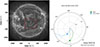 |
Fig. 1. Left: AIA 171 Å full-disc image on 2023 October 28, 14:04 UT with the ROI boxed in red. Right: Illustration from the solar-MACH tool Gieseler et al. (2023) where the location of the Earth and SDO marked by (1) and Solar Orbiter marked by (2) relative to the Sun is shown. |
The level-2 calibrated data of HRIEUV were used (preprocessing was applied to reduce spacecraft pointing errors and jitter in the images) from EUI data release 6 (Kraaikamp et al. 2023). The specific HRIEUV observation sequence we used was obtained with Solar Orbiter Observing Plan (SOOP) called R_BOTH_HRES_MCAD_Bright-Points (Auchère et al. 2020; Zouganelis et al. 2020). For AIA observations, we used calibrated level-1 scientific data from the AIA instrument that are available from the Joint Science Operations Centre (JSOC 2025), and we applied the standard AIA data-processing steps using the SSWIDL routine of aia_prep.pro.
In order to compare results from the two viewpoints, we transformed all images into Carrington coordinates. This was hard because the transformation required a mapping onto a spherical surface. When we used the photosphere as the surface, a consistent shift was seen between features in HRIEUV and AIA because the observed light is dominated by emission from the low corona above the photosphere. We therefore experimented with surfaces at different heliocentric distances that ranged from the photosphere into the corona. The images taken closest to the middle time of our period of interest (14:05UT) were used for both instruments. We varied the distance independently for both instruments because we assumed that their emission is dominant at different heights. For each pair of heights (HRIEUV height and the independent AIA height), we remapped the images onto a regular Carrington longitude and latitude grid projected to this spherical surface, and we calculated the translational Δx and Δy subpixel shifts required to maximise the spatial alignment between the images using Fourier correlation tracking (FCT, Fisher & Welsch 2008). This analysis was limited to the region of interest defined by the HRIEUV FOV because the AIA observes the full solar disc. For each pair of images, we calculated a translational shift magnitude as TSM =  . Figure 2a shows the variation in TSM as a function of height. The calculations were made at increments of ≈1.5 Mm, and the results of Figure 2 show the cubic spline interpolation of the discrete results. This surface reaches a minimum TSM of ≈1 pixel at a height of 11.4 Mm for HRIEUV and 4 Mm for AIA. Cuts of the TSM as a function of height are shown in Figures 2b and c for HRIEUV and AIA, respectively. These optimal distances defined our spherical surface for remapping into Carrington coordinates for all our subsequent results, and they enabled the best comparison of features across the ROI.
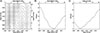 |
Fig. 2. (a) TSM or the magnitude of the translational pixel shift between the HRIEUV and AIA images after remapping to Carrington longitude-latitude coordinates as a function of height for HRIEUV (x-axis) and AIA (y-axis). These heights describe the surface we used to map to spherical coordinates, and they are shown in R⊙ and Mm. The cross shows the minimum of the surface. Panels (b) and (c) show TSM as a function of height for cuts passing through the minimum point, shown by the dotted horizontal and vertical lines in panel (a). |
This method for minimising the translational shift between images uniquely gives the approximate dominant height of emission of the 171 and 174 Å channels of AIA and HRIEUV, respectively. These optimal heights are only approximated average heights because the emission comes from a range of heights. The height of maximum emission can also vary across the region, particularly between and even within different coronal structures (i.e. QS, CH, and filament channel). The optimal heights are therefore an overall average estimate that is suitable for the whole ROI, which may lead to local differences. The TSM shown in Figure 2 therefore probably has a minimum of about one pixel and is not zero. This method applied to smaller regions in order to map the dominant height of emission in different structures leads to less stable curves than for the whole region, and it requires further development.
In simplified terms, the separation between the two spacecraft is 26°, which means that a feature extending 4 Mm above the surface introduces a parallax displacement of about 1753 km. With the rebinned AIA pixel size of 864.6 km, this corresponds to about 2 pixels. Since the effective spatial resolution of AIA is about two pixels (about 1730 km), the parallax uncertainty remains within the AIA spatial resolution. Because the source and sink regions are expected to lie in the low corona, the optimised height assumed in the alignment is biased toward the altitude of strongest emission. The large-scale structure remained unchanged over the time period we examined, so that any artificial uncertainty introduced by height differences would be static and not dynamic.
After the remapping to Carrington coordinates, Figure 3 shows a closer view of the ROI for (a) HRIEUV and (b) AIA. These regions are identified by labeling all pixels below a certain intensity threshold and keeping only continuous regions with an area larger than 2 × 104 pixels. The thresholds differed between the instruments, and there is a small difference in thresholds between the CH and filaments that allows us to distinguish them. These thresholds were found by manual inspection and trial-and-error.
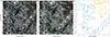 |
Fig. 3. Region of interest as observed by (a) HRIEUV and (b) AIA. For display purposes, these images were processed using MGN. The images are mapped into Carrington coordinates to better compare the features observed from the two viewpoints. The yellow contour bounds a transequatorial CH, and the filament is labelled with a cyan contour. (c) A comparison of the segmented filament and CH regions from both instruments with the filament in dark blue contours (HRIEUV) and cyan (AIA), and the CH in orange (HRIEUV) and yellow (AIA). |
It is often difficult to distinguish small CH regions near the equator from other types of regions, such as dark halo regions (e.g. Lezzi et al. 2024). The CH has been reported as such in the Heliophysics Event Knowledgebase (HEK) based on the algorithm called spatial possibilistic clustering (SPoCA, Verbeeck et al. 2014), and it seems to be a southward equatorial extension to a larger CH to the north. This northern CH and its equatorial extension is clearly visible as a dark region in AIA 193 Å images. This CH existed for several rotations prior to our date and time of study, and no identified active regions lie near the ROI for a similar time period. Figure 4 provides results from a differential emission measure (DEM) analysis of the ROI. We used all EUV channels of AIA for this analysis and applied the algorithm called solar iterative temperature emission solver (SITES) algorithm for the inversion (Morgan & Pickering 2019). To better delineate regions of different temperature, we show the fractional emission measure (FEM), which for a given pixel is the emission at a temperature divided by the total emission integrated over all temperatures, expressed as a percentage. At a low temperature of 0.8 MK, Figure 4a shows the CH as a region of relatively high FEM. The southern filament channel has a narrow central line with a relatively high FEM at this temperature. At 1.2 MK (Figure 4b), the CH FEM has dropped and the boundaries of the CH have a higher FEM. The filament has very low FEM at this ‘warm’ temperature. At higher temperatures of 1.6 MK and above (Figure 4c and d), the CH has a very low FEM. The filament has a wide strip with a high FEM at the hot temperature of 2.5 MK, which we interpret as hot plasma that surrounds the cooler filament itself that supports eclipse observations of hot prominence cavities (Habbal et al. 2010). In summary, the identification of the northwest part of the ROI as a CH is supported by this temperature analysis, its persistence over several rotations, and its association with a larger CH in the north, as described above.
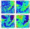 |
Fig. 4. Results of a Differential Emission Measure (DEM) analysis of the ROI at four selected temperatures (a) 0.8, (b) 1.2, (c) 1.6, and (d) 2.5 MK. These plots show the Fractional Emission Measure (FEM), which is the emission at a given temperature divided by the total emission (integrated over all temperatures) at that pixel expressed as a percentage, as shown in the colour bars. |
2.2. Time-normalised optical flow
The TNOF method works in two main steps that we summarise here, the full details are given by Morgan & Korsós (2022a) (Paper II). First, small-scale dynamics including faint PDs are enhanced through a time-normalisation process. The second step involves an optical flow algorithm to characterise any quasi-repetitive faint motions.
A time series of images of the ROI was loaded into a data cube, and the individual frames were globally co-aligned via subpixel translations found using a Fourier correlation to a central reference image taken closest to the mid-time of the observation period (Fisher & Welsch 2008). After the alignment, the images were spatially rebinned through local averaging, as discussed further below. High-frequency noise was then reduced by applying a narrow Gaussian low-pass filter to the time series of each pixel. The time series was filtered by subtracting a time-local weighted mean (calculated by convolution with a wide Gaussian kernel) and dividing by the local weighted standard deviation (calculated over the same wide kernel) plus a small constant, which produced a filtered signal with a local zero mean and a standard deviation of one. This was the time-normalisation step. The small constant avoids division by very small numbers in low-signal regions. Additional noise reduction was achieved through a spatial multi-scale à trous decomposition that discarded the highest-frequency component and summed the remaining scales (applied to each time frame independently).
In the second step, a modified Lucas-Kanade optical flow algorithm was used to derive a velocity vector field, capturing the direction and magnitude of motion in the ROI. The algorithm calculated the spatial (x and y) and temporal (t) derivatives of the intensity, and determined a least-squares solution for the velocities vx and vy at each pixel using the standard relation between the derivatives on which Lucas-Kanade is based (see Equation 4 of Paper II). We had 600 time steps at each pixel for AIA and 1400 time steps for HRIEUV, and we therefore found the least-squares solution locally at each pixel independently (the Lucas-Kanade algorithm usually operates on pairs of images and thus requires a local group of pixels for a solution). Shorter observation periods lead to less coherent velocity fields because there are fewer data points, which increases fluctuations at small scales and decreased the correlation with the coronal structure. The velocities (in units of pixels per time step) were used to warp the image intensities, which essentially reduced any motion shifts between time steps, and the process was repeated. Iteration continued until the change in the velocity field became small. There were further steps at each iteration, including imposing an adaptive local spatial smoothing on the velocities based on the fitting residuals, all detailed in Paper II. Based solely on the fitting residuals, Paper II gives an uncertainty of 6.5% on the derived velocities for a QS region in the 193 Å AIA channel. This should be considered a minimum uncertainty estimate.
After we determined the velocities, the units were converted from pixels per time step into kms−1 using the appropriate spherical coordinates of each pixel (based on the optimal heights given by the TSM approach described above). We recall that these are the plane-of-sky optical velocities that have projection effects. We minimised this by choosing a region near the disc centre and by the appropriate use of spherical coordinates at the optimal height. Changing the width of smoothing kernels resulted in different velocity magnitudes, although the vector directions remained consistent (see Section 5 of Morgan & Hutton 2018). Morgan & Hutton (2018) also reported a bias in the vx values that is consistent with the solar rotational velocity, which gives us some confidence that the optical velocities are reasonably well calibrated. In this work, the step of co-aligning the datacube images removed this bias.
For computational efficiency and improved noise statistics, we spatially rebinned the images prior to applying the TNOF method. This rebinning uses local averaging to a new image size that is an integer division of the number of original pixels. To compare the results from the two instruments with different spatial pixel scales, we also used this rebinning step to match the pixel spatial scales of the two instruments better. The closest matching pixel scales were given by integer rebinning factors of two for AIA and four for HRIEUV. For the HRIEUV sequence we used, the observed solar radius was 1851.90″ and the pixel scale was 0.49″ which is 184.8 km at the Sun. For AIA, the observed solar radius was 965.88″ and the pixel scale was 0.60″ which is 432.3 km. Therefore, the rebinned images have a pixel scale of 739.32 km for HRIEUV and 864.6 km for AIA. Table 1 shows the effect of different rebinning factors on the TNOF speed values. The mean, median, and maximum values of the speeds across the ROI are listed for HRIEUV and AIA for rebinning factors from 2 to 6. The highlighted rows show our final selection of the rebinning values based on the comparable pixel size. A higher rebinning value gives a smoother velocity field and higher speed values. When the same bin factors between the instruments are compared, AIA always has higher speeds because of the larger pixels.
Comparison of mean, median, and maximum speeds for HRIEUV and AIA for varying rebin factors.
Our results assumed a similar measurement of the plasma by the two instruments. Shestov et al. (2025) compared the temperature response of HRIEUV and the AIA channels (see, e.g. their Figures 2 and 3) and showed that the radiometric sensitivity of HRIEUV is approximately 40% higher than that of AIA 171 Å. The HRIEUV bandpass is reported to be slightly broader than the AIA 171 Å bandpass (Shestov et al. 2025; Dolliou et al. 2023), with the HRIEUV bandpass centred very close to the Fe IX/X emission, and the peak temperature response occurs at 1.0 MK. The AIA 171 Å bandpass is dominated by Fe IX, which peaks closer to 0.8 MK. HRIEUV is therefore far more sensitive to a slightly hotter plasma than AIA 171 Å. This is supported by our TSM analysis, where the optimal height for HRIEUV is considerably higher, and thus hotter, than for AIA 171 Å. The strong difference in height but relatively weak difference in temperature implies a shallow gradient of the temperature increase in the low corona for this region.
3. Results
3.1. Velocity vector fields
The velocity fields, superimposed on the background intensity images, are shown in Figure 5 for HRIEUV and AIA. For the visualisation, the field lines are plotted with a rainbow colour scheme from red, yellow, and green to blue to indicate the propagation direction, with a field line starting with red, and advancing through yellow, green, and ending in blue. The vector maps show similarities in both channels across most of the ROI, and the larger-scale coherent structures agree well. The differences might arise from projection effects inherent to the different longitudinal viewpoints, from assuming a constant height in mapping to Carrington coordinates, or from inherent differences in the data (pixel size, cadence, or noise). Some differences might also appear because of the display scheme of the vector field, that is, the field lines are traced from a random distribution of points from the TNOF results of the two nearly aligned data sequences. The different temperature response of the two instruments also causes differences.
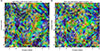 |
Fig. 5. Time-normalised optical flow velocity vector field for the (a) HRIEUV 174 Å and (b) AIA 171 Å channel. The field lines have a rainbow colour scheme to indicate propagation direction, with a field line starting in red and advancing through yellow, green, and blue. The background image is the original intensity image with MGN processing. |
Within the QS (outside of the filaments and CH), the field is typically distributed as a network of distinct cells, many of which are circular/elliptical with a typical diameter of 30–50″. There are other more elongated features, with coherent sets of field lines extending across several degrees of longitude/latitude. Many of these structures originate from a concentration of PDs sources (red line sections), but there are also concentrations of PDs sinks (blue/black sections). Long spines of converging or diverging flows often connect multiple source or sink regions, and clear, narrow boundaries are marked by very low or zero velocities.
The top row of Figure 6 shows a QS region nestled within the U-shaped filament in greater detail. There are clearly formed cells that appear in the vector maps of both instruments. For example, the source (red) cell centred at approximately (2, −11) that is labelled in the top panels clearly exists in both instruments. It appears as a point source in AIA, but as two closely separated point sources in HRIEUV. This is an example of a topological difference that is most likely due to the different spatiotemporal resolutions, sensitivity, and temperature sensitivity of the instruments. We expect the magnetic topology to vary between the different emission heights viewed by the two instruments. The cell centre in HRIEUV at coordinates (−2, −13) has an elongated sink (blue) region. The flow lines converge from all directions into this elongated sink. In AIA, this feature appears to be shifted east by half a degree in longitude (to the left). This pattern of consistent features that are shifted by a small factor in coordinates between the instrument likely has two main reasons. (1) The global heights to the spherical surface for the mapping to Carrington coordinates might not be suitable for all regions. (2) The topology of the magnetic field might change between the dominant height layer observed by AIA and HRIEUV.
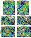 |
Fig. 6. Greater detail of the selected subregions showing QS (top), part of a filament (middle), and the CH (bottom). |
The U-shaped filament structure is dominated by blue lines, indicating that PDs end their propagation within the filament. The middle row of Figure 6 shows a closer view of part of a filament located in the top left corner of Figure 5. The field lines are generally aligned along the filament spine, with a predominant single direction of motion. Thus, PDs tend to propagate from closely neighbouring QS regions into the filament, at which point they propagate along the filament in a consistent direction. This is seen in both instruments, although there are some differences in the actual detail at smaller scales for the same reasons as listed above.
The equatorial CH shows the interesting feature of very long coherent velocity field lines that form a bridge from one side of the CH to the other (from left to right). This is shown in more detail in the bottom row of Figure 6. These field lines originate from the QS east (left) of the CH and extend west across to the QS (right). These are the longest coherent field lines throughout the ROI, and they are structurally different from the line of the QS and the filaments in that they do not exhibit a cell-like pattern. The intensity images of Figure 5 show few faint approximately linear enhancements in the intensity bridging across the CH with a similar configuration as the PD velocity field lines. The velocity field must therefore arise from PDs traversing along a QS magnetic field that forms a bridge across the CH. This contrast with the expected open magnetic field topology of CHs. The intensity images only show a few loops that form bridges across the CH, whilst the velocity field suggests that this is a general configuration in the whole CH.
3.2. Speed distributions
Figure 7 maps the TNOF speeds for both instruments. The CH appears as a broad region with a higher speed in the 20–40 kms−1 range for both instruments. Outside of the CH lie only isolated regions with higher speeds, and most of the regions have values of below 10 kms−1 or close to the most probable speed of about 5 kms−1. The speeds in the filament channel do not show the coherence of the CH, although clusters of higher speeds are distributed along the boundaries of the southern U-shaped bend of the filament. Overall, our optical velocities are in the expected range of slow MA waves, and they agree with previous reports (e.g. Nakariakov & Zimovets 2011; Zhao et al. 2025; De Moortel et al. 2014; Gupta et al. 2012).
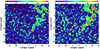 |
Fig. 7. Time-normalised optical flow speeds over the ROI for HRIEUV (left) and AIA (right). The maps have the same colour scale as in the colour bars above each plot. |
The left panel of Figure 8 compares the distribution of speeds across the whole ROI for both instruments. The distributions are very similar. Both extend to velocities up to approximately 40 kms−1. AIA has a mean of 9.02 kms−1 and the mean of HRIEUV is 10.14 kms−1. The most probable speed for AIA is 4.0 kms−1, compared to 4.8 kms−1 for HRIEUV. The middle and right panels of Figure 8 compare the AIA and HRIEUV distribution of the x (longitudinal) and y (latitudinal) velocity components in the whole ROI. The most probable Vx speed is 1.5 kms−1 for AIA and −1.6 kms−1 for HRIEUV, and for Vy, the most probable speed for both AIA and HRIEUV is −1.4 kms−1. The small difference in Vx might be due to the optimal height for the conversion to spherical coordinates, although this is also expected to lead to a small difference in the y component. A more subtle effect might arise from an early step in the method in which successive image frames are aligned by a global translational shift in x and y. This global alignment fits successive images best, but it might not be accurate for the entire ROI because different areas are expected to shift by different quantities (due to the spherical geometry and differential rotation). The same effect is present in AIA and HRIEUV, but is stronger in AIA because of the faster apparent rotation of the Sun due to the spacecraft orbital dynamics. This effect will always be most apparent in the longitudinal velocity component.
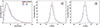 |
Fig. 8. Left panel: Distribution of TNOF speeds across the whole ROI for AIA (red) and HRIEUV (blue). Middle and right panels: x (middle) and y (right) velocity components for both instruments. |
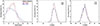 |
Fig. 9. Left panel: Histogram of speeds (left), and x (middle) and y (right) velocity components in the CH region for AIA (red) and HRIEUV (blue). |
Figure 10 shows histograms of the filament region speeds for AIA (red) and HRIEUV (blue). The two distributions agree very closely. The speeds peak at values near 5 kms−1 and the distributions decline to about 25–30 kms−1. These speeds are considerably lower than the CH. The x and y speed components in the middle and right panel agree well, with the largest difference seen in the x component of the middle panel. Here, HRIEUV is shifted to slightly higher positive values. Similar to the CH, this might be due to the different sensitivity of the instruments and other effects, but it might also be due to the projected true velocities seen from the different longitudinal viewpoints.
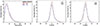 |
Fig. 10. Left panel: Histogram of speeds for the filament region for AIA (red) and HRIEUV (blue). Middle and right panels: The x (middle) and y (right) components for both instruments. |
Figure 11 shows speed histograms in the quiet-Sun regions (i.e. not belonging to the CH or filament) for AIA (red) and HRIEUV (blue). The two distributions agree very closely. The speeds peak at values in AIA of 2.30 kms−1 and 4.60 kms−1 for HRIEUV and distributions decline to around 30 kms−1. The mean speed for AIA is 8.23 kms−1 and 9.25 kms−1. These speeds are considerably lower than those in the CH and are slightly lower than the filament. Again, the x and y speed components in the middle and right panel agree well, with a small difference in the x component of the middle panel. Here, HRIEUV is shifted to slightly higher positive values. Similar to the previous histograms, this might be due to the different sensitivity of the instruments and other effects, but it might also be due to the projected true velocities seen from the different longitudinal viewpoints.
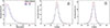 |
Fig. 11. Left panel: Histogram of speeds for the quiet-Sun region for AIA (red) and HRIEUV (blue). Middle and right panels: x (middle) and y (right) components for the two instruments. |
4. Discussion
The CH is a large region with consistently higher speeds than in the rest of the ROI. This is probably linked to the system of linear magnetic loops that form bridges across the CH that might be conducive to these high speeds compared to the smaller systems of loops in the QS. Alternatively or in addition, these loops might be rooted in QS network regions with a higher magnetic field strength that might drive faster PDs, although other loop systems in the QS are rooted in photospheric network regions with a similar strength and show no such high speeds.
Figure 12 shows field lines from a potential field (PF) model overlaid on a HMI magnetogram with the model limited to a region encompassing the CH. The model was created using Green’s function and considered all pixels from a magnetogram region, with margins extending beyond the model volume. HMI shows that photospheric positive polarities are slightly dominant in this whole region (CH and QS), with a mean field of 3.2G. The photospheric field strength within the CH is slightly lower than the surrounding QS region (8.3G compared to 9.0G) and has a higher excess positive flux (mean field of 5.0G compared to 2.9G for the QS). Whilst some local opposite polarities are linked by smaller loops, there are systems of overlying field lines that are long and link more distant regions, including field lines that extend across the CH. This generally agrees with the TNOF velocity map of Figure 5. Although a PF extrapolation of this limited region containing generally weak field (i.e. with a higher relative uncertainty in the photospheric measurement) is not likely to give a wholly accurate model of the coronal field, Figure 12 supports our interpretation of the coronal field above the CH.
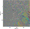 |
Fig. 12. Magnetic field lines from a PF model of the HMI observed photospheric field for a region encompassing the CH. The background image is the HMI observation, and positive (negative) regions are shown in white (black). The CH is bounded in pink and part of the filament channel in orange. The colour along a field line represents the height above the photosphere and ranges from black (low height) through blue, green, yellow, and red for an increasing height to the limit of the model volume at ∼0.1 R⊙. |
This CH is old (it persisted for several solar rotations prior to these observations) and narrow in longitudinal extent, as is typical of small equatorial CHs. The closed magnetic field from the surrounding QS regions might evolve through gradual small-scale reconnection with the open field so that it eventually forms a bridge across the CH. This implies that the CH might not possess an open field. The question then arises why it appears so clearly as a dark low-temperature region in the EUV. The properties of the plasma are typical of a CH, but the magnetic field properties are not.
The left panel of Figure 9 shows significant differences between the HRIEUV and AIA speed distributions within the CH. The reason might be the spatiotemporal resolution and sensitivity, as described previously. Another possibility is the effect of the projected true PD velocities in the corona to the different image planes of the instruments. This projection effect would be difficult to see in the QS or filament because of its smaller-scale structure and complexity, but it is expected to be most apparent in a region such as this CH, with its system of coherent linear motion lines throughout a broad region. The CH is closer to the disc centre for AIA than for HRIEUV and is subject to fewer projection effects. Furthermore, the projection effect is stronger in the longitudinal than in the latitudinal dimension. This argument supports the greater difference in the mean speeds of the instruments in the longitudinal (x) direction compared to the latitudinal (y) direction.
Another effect might be the different height of the peak emission of the two instruments. Previous works using TNOF showed clear topological differences in the velocity fields from different AIA channels, which are dominated by different temperatures/heights in the atmosphere. For example, the 304 Å channel shows a smaller-scale cell-like pattern than the 171 Å and 193 Å channels. The 193 Å channel in particular shows the largest coherent cell-like structures. We expect the magnetic topology, as well as the PDs speeds, to change between the 4 Mm AIA 171 Å height and the 11.4 Mm HRIEUV 174 Å height. The challenge is to distinguish these real topological features from other effects, and this will require further development.
Figure 5 shows that the dominant colour of the velocity field lines within the FC is blue to black, which means that most PDs velocity vectors start near the filament channel boundary and end within the filament. This suggests that PD activity in filaments is dominated by external drivers, although the core of the filament is likely cool and optically thick and will not be seen in our observations. These are elongated field lines that tend to align approximately along the filament spine. This pattern of PDs propagation is consistent with the expected large-scale magnetic field topology of filaments, where field lines rooted close to the filament channel enter the flux tube of the filament and become aligned with the overall flux tube axis. The lower right portion of Figure 12 shows a large arcade of PF field lines that form a bridge over part of the filament channel (outlined in orange), with the field lines approximately perpendicular to the alignment of the channel. This strongly disagrees with the filament-aligned PDs velocity field lines and shows that a PF model cannot accurately depict the highly non-potential magnetic field of a filament.
Regions outside of the CH and FC that we labelled QS are thought to consist of loop systems lying low in the corona. We have shown previously that the cell-like patterns covering QS regions are closely aligned with the photospheric network, with the network generally associated with PD sources. This agrees with the generally accepted model that the QS loop footpoints are embedded within the network. Whilst the TNOF velocity vector fields contain topological differences at smaller scales, the distribution of QS speeds are very similar. This suggests either that PDs speeds are similar over a range of low coronal heights in the QS or that the motions are most apparent in the temperature band that is common to both instruments. Future instruments with a finer temperature resolution are required to answer these questions.
5. Conclusions and future work
Our comparison of the PDs velocity fields and speeds gained from HRIEUV 174 Å and AIA 171 Å observations agrees very well overall, which increases our confidence that the TNOF method estimates the motions of PDs in the low corona accurately. We interpret the differences in PDs speeds and velocity vector maps in terms of the real variation expected with height in the corona, with the different temperature sensitivity of the instruments viewing different layers. This interpretation is limited, however, because it is currently impossible to distinguish this from other effects, such as differences in the spatiotemporal instrument resolution, projection effects due to the different viewpoints, and uncertainties in the results.
To enable the comparisons in this work, we remapped them to Carrington coordinates and optimised the heights of the spherical surfaces we used as a coordinate basis for each instrument, where we found optimised heights of 11.4 Mm for HRIEUV 174 Å and 4 Mm for AIA 171 Å. This is a large difference in height for a relatively small difference in temperature sensitivity, which implies that the gradient of the temperature height is gradual in the quiet low corona. This method can be readily applied to other suitable EUI and AIA datasets. We wish to apply this approach to smaller regions to map the height of dominant emission over different types of coronal structures. Currently, our attempts at this localised mapping give unstable results, and further development is therefore required.
The TNOF velocity vector map shows that the CH has a system of low-lying closed magnetic field that forms bridges from east to west and is rooted in nearby QS regions. This is supported by a PF magnetic model extrapolation of the observed photospheric field. This contradicts the general CH model of an open magnetic field. The CH region has consistently higher speeds than the QS and FC, which suggests that longer quasi-linear magnetic loops allow higher PDs speeds than the smaller loop systems of the QS and FC.
The configuration of the FC velocity vector field agrees with the generally accepted model of the highly non-potential tubular magnetic field of a filament, which the PF magnetic model fails to replicate. We also presented evidence that the PDs activity in filaments arises from external drivers. The QS shows a similar cell-like structure as the velocity field, which we showed previously is aligned with the photospheric network. The PD speed distributions in QS and FC regions are very similar in HRIEUV and AIA, which suggests that either PDs speeds do not vary much with height or that the instrument observations are dominated by the same layer.
A long-term goal is to use different spacecraft viewpoints to enable a three-dimensional constraint on the PDs velocity fields, but this is challenging. When the longitudinal separation is suitable, the application of TNOF to the same region from both perspectives might allow us to assess the variation in the velocity fields with viewing angle. This will help us to determine the extent to which the differences reflect the magnetic field alignment, particularly above network boundaries, and whether this approach can provide practical constraints on the field connectivity despite the uncertainties in height and projection. Another approach includes the comparison of spectral Doppler measurements and numerical simulations. Depending on their nature, the PDs might not always show a Doppler shift. The source and sink regions might still carry significant flows that are field aligned, however, which complement the TNOF PD velocity fields that show the plane-of-sky component. This type of analysis would offer a novel and valuable insight into the magnetic field topology.
Acknowledgments
We acknowledge support from Aberystwyth University through the Aberdoc PhD scholarship scheme and the President’s award. We acknowledge the support of the Royal Observatory of Belgium’s Solar Physics team through the 2024 Guest Investigator Program, which supported this research via access to the EUI data PI team in Brussels. We thank Sarah Willems and Koen Stegen for their help with IDL and Solar Soft. H. Morgan conducted work for this study under STFC grant WT414417-01. N.Narang acknowledges funding from the Belgian Federal Science Policy Office (BELSPO) contract B2/223/P1/CLOSE-UP. The SDO data used in this paper is courtesy of NASA/SDO and the AIA, EVE, and HMI science teams. Solar Orbiter is a space mission of international collaboration between ESA and NASA, operated by ESA. The EUI instrument was built by CSL, IAS, MPS, MSSL/UCL, PMOD/WRC, ROB, LCF/IO with funding from the Belgian Federal Science Policy Office (BELSPO/PRODEX PEA 4000112292 and 4000134088); the Centre National d’Etudes Spatiales (CNES); the UK Space Agency (UKSA); the Bundesministerium für Wirtschaft und Energie (BMWi) through the Deutsches Zentrum für Luft- und Raumfahrt (DLR); and the Swiss Space Office (SSO). This research used the Heliophysics Event Knowledge database and the ESA JHelioviewer.
References
- Anusha, L. S., Solanki, S. K., Hirzberger, J., & Feller, A. 2017, A&A, 598, A47 [NASA ADS] [CrossRef] [EDP Sciences] [Google Scholar]
- Auchère, F., Andretta, V., Antonucci, E., et al. 2020, A&A, 642, October 2020 The Solar Orbiter mission [Google Scholar]
- Banerjee, D., Teriaca, L., Gupta, G. R., et al. 2009, A&A, 499, L29 [NASA ADS] [CrossRef] [EDP Sciences] [Google Scholar]
- Banerjee, D., Prasad, S. K., Pant, V., et al. 2021, Space Sci. Rev., 217 [Google Scholar]
- Barczynski, K., Harra, L., Schwanitz, C., et al. 2023, A&A, 673, A74 [NASA ADS] [CrossRef] [EDP Sciences] [Google Scholar]
- Baso, D., González, M. J. M., & Ramos, A. A. 2019, A&A, 625 [Google Scholar]
- Baweja, U., Pant, V., Krishna Prasad, S., et al. 2025, arXiv e-prints [arXiv:2509.07796] [Google Scholar]
- Beck, C., & Rezaei, R. 2009, A&A, 502, 969 [NASA ADS] [CrossRef] [EDP Sciences] [Google Scholar]
- Bellot Rubio, L., & Orozco Suarez, D. 2019, Liv. Rev. Sol. Phys., 16 [Google Scholar]
- Berghmans, D., McKenzie, D., & Clette, F. 2001, A&A, 369, 291 [NASA ADS] [CrossRef] [EDP Sciences] [Google Scholar]
- Berghmans, D., Auchère, F., Long, D. M., et al. 2021, A&A, 656, L4 [NASA ADS] [CrossRef] [EDP Sciences] [Google Scholar]
- Chitta, L. P., Solanki, S. K., Peter, H., et al. 2021, A&A, 656, L13 [NASA ADS] [CrossRef] [EDP Sciences] [Google Scholar]
- Chitta, L. P., Zhukov, A. N., Berghmans, D., et al. 2023, Science, 381, 867 [NASA ADS] [CrossRef] [Google Scholar]
- Cranmer, S. R. 2009, Liv. Rev. Sol. Phys., 6 [Google Scholar]
- De Moortel, I. 2009, Space Sci. Rev., 149, 65 [Google Scholar]
- De Moortel, I., Antolin, P.,& Van Doorsselaere, T. 2014, Sol. Phys., 290, 399 [Google Scholar]
- Diercke, A., Kuckein, C., Verma, M., & Denker, C. 2018, A&A, 611, A64 [NASA ADS] [CrossRef] [EDP Sciences] [Google Scholar]
- Dolliou, A., Parenti, S., Auchère, F., et al. 2023, A&A, 671, A64 [NASA ADS] [CrossRef] [EDP Sciences] [Google Scholar]
- Fisher, G. H., & Welsch, B. 2008, arXiv e-prints [arXiv:0712.4289] [Google Scholar]
- Gieseler, J., Dresing, N., Palmroos, C., et al. 2023, Front. Astron. Space Sci., 9 [Google Scholar]
- Gissot, S., Auchère, F., Berghmans, D., et al. 2026, A&A, in press, https://doi.org/10.1051/0004-6361/202451804 [Google Scholar]
- Gupta, G. R., Teriaca, L., Marsch, E., Solanki, S. K., & Banerjee, D. 2012, A&A, 546, A93 [NASA ADS] [CrossRef] [EDP Sciences] [Google Scholar]
- Habbal, S. R., Druckmüller, M., Morgan, H., et al. 2010, ApJ, 719, 1362 [NASA ADS] [CrossRef] [Google Scholar]
- Harra, L., Barczynski, K., Auchère, F., et al. 2025, Space Sci. Rev., 221 [Google Scholar]
- Huang, Z., Madjarska, M. S., Doyle, J. G., & Lamb, D. A. 2012, A&A, 548, A62 [NASA ADS] [CrossRef] [EDP Sciences] [Google Scholar]
- Hutton, J., & Morgan, H. 2015, ApJ, 813, 35 [Google Scholar]
- JSOC. 2025, Joint Science Operations Center (JSOC) Data Products [Google Scholar]
- Khomenko, E., Collados, M., Solanki, S. K., Lagg, A., & Bueno, J. T. 2003, A&A, 408, 1115 [NASA ADS] [CrossRef] [EDP Sciences] [Google Scholar]
- Kolotkov, D. Y., Zavershinskii, D. I., & Nakariakov, V. M. 2021, Plasma Phys. Control. Fusion, 63, 124008 [CrossRef] [Google Scholar]
- Kraaikamp, E., Gissot, S., Stegen, K., et al. 2023, SolO/EUI Data Release 6.0 2023-01, https://doi.org/10.24414/z818-4163, published by Royal Observatory of Belgium (ROB) [Google Scholar]
- Kuckein, C., Verma, M., & Denker, C. 2016, A&A, 589, A84 [NASA ADS] [CrossRef] [EDP Sciences] [Google Scholar]
- Lemen, J. R., Title, A. M., Akin, D. L., et al. 2012, Sol. Phys., 275, 17 [Google Scholar]
- Lezzi, S. M., Andretta, V., Murabito, M., & Del Zanna, G. 2023, A&A, 680, A61 [NASA ADS] [CrossRef] [EDP Sciences] [Google Scholar]
- Lezzi, S. M., Long, D. M., Andretta, V., et al. 2024, A&A, 690, A342 [NASA ADS] [CrossRef] [EDP Sciences] [Google Scholar]
- Lim, D., Van Doorsselaere, T., Berghmans, D., et al. 2025, A&A, 698, A65 [NASA ADS] [CrossRef] [EDP Sciences] [Google Scholar]
- Meadowcroft, R. L., Zhong, S., Kolotkov, D. Y., & Nakariakov, V. M. 2023, MNRAS, 527, 5302 [NASA ADS] [CrossRef] [Google Scholar]
- Morgan, H., & Druckmüller, M. 2014, Sol. Phys., 289, 2945 [Google Scholar]
- Morgan, H., & Hutton, J. 2018, ApJ, 853, 145 [Google Scholar]
- Morgan, H., & Korsós, M. 2022a, Sol. Phys., 297, 102 [NASA ADS] [CrossRef] [Google Scholar]
- Morgan, H., & Korsós, M. B. 2022b, ApJ, 933, L27 [Google Scholar]
- Morgan, H., & Pickering, J. 2019, Sol. Phys., 294, 135 [NASA ADS] [CrossRef] [Google Scholar]
- Morgan, H., & Taroyan, Y. 2017, Sci. Adv., 3 [Google Scholar]
- Müller, D., St. Cyr, O. C., Zouganelis, I., et al. 2020, A&A, 642, A1 [Google Scholar]
- Nakariakov, V. M., & Zimovets, I. V. 2011, ApJ, 730, L27 [Google Scholar]
- Narang, N., Verbeeck, C., Mierla, M., et al. 2025, A&A, 699, A138 [NASA ADS] [CrossRef] [EDP Sciences] [Google Scholar]
- O’Shea, E., Banerjee, D., & Doyle, J. G. 2006, A&A, 463, 713 [Google Scholar]
- Pesnell, D., & Addison, K. 2011, SDO | Solar Dynamics Observatory [Google Scholar]
- Rochus, P., Auchère, F., Berghmans, D., Harra, L., et al. 2020, A&A, 642, A8 [NASA ADS] [CrossRef] [EDP Sciences] [Google Scholar]
- Schwanitz, C., Harra, L., Barczynski, K., et al. 2023a, Sol. Phys., 298 [Google Scholar]
- Schwanitz, C., Harra, L., Mandrini, C. H., et al. 2023b, A&A, 674, A219 [NASA ADS] [CrossRef] [EDP Sciences] [Google Scholar]
- Shestov, S. V., Zhukov, A. N., Auchère, F., Berghmans, D., & Loicq, J. 2025, A&A, 699, A7 [NASA ADS] [CrossRef] [EDP Sciences] [Google Scholar]
- Somaiyeh, S., & Poedts, S. 2024, Sci. Rep., 14 [Google Scholar]
- Stankovic, N., & Morgan, H. 2025, Sol. Phys., 300 [Google Scholar]
- Suárez, D. O., & Bellot, R. 2012, ApJ, 751, 2 [Google Scholar]
- Tian, H., McIntosh, S. W., & Pontieu, B. D. 2011, ApJ, 727, L37 [NASA ADS] [CrossRef] [Google Scholar]
- van Driel-Gesztelyi, L. 2006, Proc. Int. Astron. Union, 2, 205 [Google Scholar]
- van Driel-Gesztelyi, L., Culhane, J. L., Baker, D., et al. 2012, Sol. Phys., 281, 237 [Google Scholar]
- Verbeeck, C., Delouille, V., Mampaey, B., & De Visscher, R. 2014, A&A, 561, A29 [NASA ADS] [CrossRef] [EDP Sciences] [Google Scholar]
- Wang, Y.-M. 2008, Space Sci. Rev., 144, 383 [Google Scholar]
- Wiegelmann, T., & Solanki, S. K. 2004, Sol. Phys., 225, 227 [NASA ADS] [CrossRef] [Google Scholar]
- Zhao, J., Wang, T., & Chen, R. 2025, MNRAS, 538, 797 [Google Scholar]
- Zouganelis, I., Groof, A. D., Walsh, A. P., et al. 2020, A&A, 642, A3 [NASA ADS] [CrossRef] [EDP Sciences] [Google Scholar]
All Tables
Comparison of mean, median, and maximum speeds for HRIEUV and AIA for varying rebin factors.
All Figures
|
Fig. 1. Left: AIA 171 Å full-disc image on 2023 October 28, 14:04 UT with the ROI boxed in red. Right: Illustration from the solar-MACH tool Gieseler et al. (2023) where the location of the Earth and SDO marked by (1) and Solar Orbiter marked by (2) relative to the Sun is shown. |
| In the text | |
|
Fig. 2. (a) TSM or the magnitude of the translational pixel shift between the HRIEUV and AIA images after remapping to Carrington longitude-latitude coordinates as a function of height for HRIEUV (x-axis) and AIA (y-axis). These heights describe the surface we used to map to spherical coordinates, and they are shown in R⊙ and Mm. The cross shows the minimum of the surface. Panels (b) and (c) show TSM as a function of height for cuts passing through the minimum point, shown by the dotted horizontal and vertical lines in panel (a). |
| In the text | |
|
Fig. 3. Region of interest as observed by (a) HRIEUV and (b) AIA. For display purposes, these images were processed using MGN. The images are mapped into Carrington coordinates to better compare the features observed from the two viewpoints. The yellow contour bounds a transequatorial CH, and the filament is labelled with a cyan contour. (c) A comparison of the segmented filament and CH regions from both instruments with the filament in dark blue contours (HRIEUV) and cyan (AIA), and the CH in orange (HRIEUV) and yellow (AIA). |
| In the text | |
|
Fig. 4. Results of a Differential Emission Measure (DEM) analysis of the ROI at four selected temperatures (a) 0.8, (b) 1.2, (c) 1.6, and (d) 2.5 MK. These plots show the Fractional Emission Measure (FEM), which is the emission at a given temperature divided by the total emission (integrated over all temperatures) at that pixel expressed as a percentage, as shown in the colour bars. |
| In the text | |
|
Fig. 5. Time-normalised optical flow velocity vector field for the (a) HRIEUV 174 Å and (b) AIA 171 Å channel. The field lines have a rainbow colour scheme to indicate propagation direction, with a field line starting in red and advancing through yellow, green, and blue. The background image is the original intensity image with MGN processing. |
| In the text | |
|
Fig. 6. Greater detail of the selected subregions showing QS (top), part of a filament (middle), and the CH (bottom). |
| In the text | |
|
Fig. 7. Time-normalised optical flow speeds over the ROI for HRIEUV (left) and AIA (right). The maps have the same colour scale as in the colour bars above each plot. |
| In the text | |
|
Fig. 8. Left panel: Distribution of TNOF speeds across the whole ROI for AIA (red) and HRIEUV (blue). Middle and right panels: x (middle) and y (right) velocity components for both instruments. |
| In the text | |
|
Fig. 9. Left panel: Histogram of speeds (left), and x (middle) and y (right) velocity components in the CH region for AIA (red) and HRIEUV (blue). |
| In the text | |
|
Fig. 10. Left panel: Histogram of speeds for the filament region for AIA (red) and HRIEUV (blue). Middle and right panels: The x (middle) and y (right) components for both instruments. |
| In the text | |
|
Fig. 11. Left panel: Histogram of speeds for the quiet-Sun region for AIA (red) and HRIEUV (blue). Middle and right panels: x (middle) and y (right) components for the two instruments. |
| In the text | |
|
Fig. 12. Magnetic field lines from a PF model of the HMI observed photospheric field for a region encompassing the CH. The background image is the HMI observation, and positive (negative) regions are shown in white (black). The CH is bounded in pink and part of the filament channel in orange. The colour along a field line represents the height above the photosphere and ranges from black (low height) through blue, green, yellow, and red for an increasing height to the limit of the model volume at ∼0.1 R⊙. |
| In the text | |
Current usage metrics show cumulative count of Article Views (full-text article views including HTML views, PDF and ePub downloads, according to the available data) and Abstracts Views on Vision4Press platform.
Data correspond to usage on the plateform after 2015. The current usage metrics is available 48-96 hours after online publication and is updated daily on week days.
Initial download of the metrics may take a while.