| Issue |
A&A
Volume 706, February 2026
|
|
|---|---|---|
| Article Number | A258 | |
| Number of page(s) | 10 | |
| Section | Planets, planetary systems, and small bodies | |
| DOI | https://doi.org/10.1051/0004-6361/202557711 | |
| Published online | 17 February 2026 | |
Observations of counter-streaming ions in and around the diamagnetic cavity of comet 67P
1
School of Earth and Space Science and Technology, Wuhan University,
430072
Wuhan,
China
2
Swedish Institute of Space Physics,
Box 812,
981 28
Kiruna,
Sweden
3
Division of Space and Plasma Physics, School of Electrical Engineering and Computer Science, KTH Royal Institute of Technology,
114 28
Stockholm,
Sweden
★ Corresponding author: This email address is being protected from spambots. You need JavaScript enabled to view it.
Received:
15
October
2025
Accepted:
5
January
2026
Abstract
Context. Ion speeds at comet 67P/Churyumov-Gerasimenko significantly exceed local neutral gas speeds, a discrepancy that challenges current ion-neutral coupling models. The presence of counter-streaming ion populations is a proposed solution, as it can reconcile high individual velocities with a low bulk flow speed and potentially drive wave activity through ion-ion instabilities.
Aims. We aim to identify and statistically characterize counter-streaming ion populations to provide the first quantitative constraints on this phenomenon.
Methods. We analyzed high- and standard-resolution data from the Ion Composition Analyser (ICA), part of the Rosetta Plasma Consortium (RPC) on board the Rosetta spacecraft. The events were selected from periods when Rosetta was inside or near the diamagnetic cavity, a key region for cometary plasma dynamics.
Results. A total of 112 events are identified in the high-resolution data and 338 in the standard-resolution data, both inside and outside the diamagnetic cavity. In general, the anticometward ion population exhibits higher energy and particle counts compared to the cometward ion population. The angular separation between the two flows is peaked in the range of 150°–180°. The superposition of these high-speed flows produce net bulk velocities of a few km/s.
Conclusions. Our findings provide statistical evidence of counter-streaming ions at a comet and demonstrate that they can lead to a low net bulk speed. Return flows can be explained by gyration of the ions in the magnetic field just outside the diamagnetic cavity.
Key words: magnetic fields / plasmas / methods: observational / methods: statistical / comets: general / comets: individual: 67P/Churyumov-Gerasimenko
© The Authors 2026
 Open Access article, published by EDP Sciences, under the terms of the Creative Commons Attribution License (https://creativecommons.org/licenses/by/4.0), which permits unrestricted use, distribution, and reproduction in any medium, provided the original work is properly cited.
This article is published in open access under the Subscribe to Open model. This email address is being protected from spambots. You need JavaScript enabled to view it. to support open access publication.
1 Introduction
Comets are relics from the dawn of our planetary system. They carry fundamental clues about the formation and primordial composition of the Solar System (Altwegg et al. 2019). When these icy bodies approach the Sun, their surface materials sublimate to form an extensive neutral atmosphere, the coma (e.g., Lamy et al. 1998; Lisse et al. 2005; Nilsson et al. 2015). The outgassed material subsequently interacts with the solar wind and the Sun’s extreme ultraviolet (EUV) radiation, creating a complex and dynamic plasma environment (Goetz et al. 2022) through processes of photoionization, electron-impact ionization, and charge exchange (Biermann et al. 1967; Galand et al. 2016; Simon Wedlund et al. 2017). For decades, the direct exploration of this environment was restricted to brief flybys. This limitation was overcome by the European Space Agency (ESA) Rosetta mission, which orbited comet 67P/Churyumov-Gerasimenko (67P/C-G) from 2014 to 2016 (Glassmeier et al. 2007a). The mission delivered the first-ever, long-term in situ measurements from deep within the coma. The plasma instrument package provided by the Rosetta Plasma Consortium (RPC; Carr et al. 2007) has revolutionized our understanding of the large-scale comet-solar wind interaction (Broiles et al. 2015; Edberg et al. 2016; Glassmeier 2017), while also revealing an unexpected complexity of fine structures (e.g., Goetz et al. 2016a,b; Stenberg Wieser et al. 2017; Ostaszewski et al. 2021).
The diamagnetic cavity is a region of the near-zero magnetic field that forms around the nucleus of an active comet (Neubauer et al. 1986; Goetz et al. 2016a). Its existence is a direct consequence of the solar wind’s interaction with the expanding cometary atmosphere. The solar wind carries the interplanetary magnetic field (IMF) through the dense neutral gas of the coma. As this magnetized plasma moves, it continuously assimilates newly formed, heavy cometary ions. This process, known as mass loading, causes the plasma to deflect and decelerate before it can reach the nucleus (e.g., Wallis 1973; Szegö et al. 2000; Behar et al. 2016a,b). When the outgassing from the nucleus is large enough, the diamagnetic cavity is formed. While the diamagnetic cavity seen at 1P/Halley was large and stable (Neubauer 1988), the cavity at 67P was intermittent and unstable (Goetz et al. 2016a; Henri et al. 2017). The size and distance of its boundary were governed by long-term trends in the outgassing rate and the solar wind dynamic pressure (Goetz et al. 2016b; Timar et al. 2017). Investigating the plasma in and around this region is therefore crucial for understanding the formation of the cavity boundary and the dynamics of the cometary plasma, unperturbed by the direct influence of the solar wind (Israelevich et al. 1992; Hajra et al. 2018; Odelstad et al. 2018; Masunaga et al. 2019).
Nemeth et al. (2016) reported sharp dropouts in the suprathermal electron population (100–200 eV) near the cavity, interpreted as field-aligned electrons being excluded from the unmagnetized region. Concurrently, the energetic ion bursts have been observed, pointing to local acceleration mechanisms (Stenberg Wieser et al. 2017; Masunaga et al. 2019). Knowledge of both the initial low-energy cometary ion flow and the accelerated energetic particles is important to understand the dynamics. Modeling and theoretical studies suggest an initial outward flow of low-energy ions driven by the ambipolar electric field (Koenders et al. 2015; Vigren & Eriksson 2017, 2019). These ions may be reflected at the diamagnetic cavity boundary (Puhl-Quinn & Cravens 1995). However, there are no observational reports of the initial, newborn low-energy ion population (<20 eV) traveling away from the nucleus (Bergman et al. 2021a). Low-energy ions (<20 eV) are observed flowing back toward the nucleus, whereas accelerated ions with higher energies move away from the comet and possess an antisunward component (Bergman et al. 2021a).
Typically, a newly formed ion is assumed to inherit the velocity of its parent neutral molecule, which is ~0.5–1 km/s (Gulkis et al. 2015). This assumption holds true reasonably well when modeling the cometary environment at low outgassing rates, successfully reproducing observed electron densities at larger heliocentric distances (Galand et al. 2016; Heritier et al. 2017). However, this simple picture breaks down near perihelion (Vigren et al. 2019). Models that neglect ion acceleration significantly overestimate the plasma densities measured inside the diamagnetic cavity. To match the observed density profiles, recent modeling indicates that ions must be transported away with an accelerated bulk speed of 1.2–3 km/s, faster than the neutral gas (Lewis et al. 2024).
In contrast to the relatively modest speeds required by models, in situ observations reveal a complex picture of ion velocities. Analyses combining data from Langmuir probes (RPC-LAP; Eriksson et al. 2007) and the Mutual Impedance Probe (RPC-MIP; Trotignon et al. 2007) suggest effective ion speeds in the range of 2–8 km/s (Vigren et al. 2017; Odelstad et al. 2018). These LAP-derived speeds are inferred from current voltage characteristics under the assumption of a single, drifting Maxwellian population. This assumption makes the interpretation ambiguous if multiple ion populations are present. In contrast, the Ion Composition Analyser (PPC-ICA; Nilsson et al. 2007) offers a more direct approach by measuring the ion distribution itself. Detailed investigation of these data reveals even higher bulk speeds, in the range of 5–10 km/s (Bergman et al. 2021b).
To reconcile the low bulk velocity required by models with the high speeds observed for individual ions, a leading hypothesis proposes the existence of two counter-streaming ion populations (Bergman et al. 2021a). One of these streams corresponds to the theoretically necessary but still unobserved outward low-energy flow. Such a counter-streaming configuration provides a natural source of free energy that can drive plasma instabilities. This offers a mechanism for generating plasma waves frequently observed in and around the diamagnetic cavity (Gunell et al. 2017; Madsen et al. 2018; Ostaszewski et al. 2021).
In the present study, we survey the ion data observed by Rosetta for evidence of counter-streaming low-energy ion populations and characterize the events we identify. The structure of the paper is as follows: Section 2 describes the instrumentation, database construction, and event analysis method. Section 3 presents the observations and the statistical results. The discussion and conclusion are provided in Sections 4 and 5, respectively.
2 Instrumentation and data analysis
2.1 The Rosetta plasma consortium (RPC) instruments
The Rosetta Plasma Consortium (RPC) is a suite of five instruments designed for in situ measurements of the plasma environment of comet 67P (Carr et al. 2007). In this study, we specifically use data from the Ion Composition Analyser (RPC-ICA; Nilsson et al. 2007), the Magnetometer (RPC-MAG; Glassmeier et al. 2007b), and the Langmuir Probes (RPC-LAP; Eriksson et al. 2007).
RPC-ICA is a mass resolving ion spectrometer, which provides measurements of the ion composition and velocity distribution function. Its field of view covers 360° in azimuth and ±45° in elevation, divided into 16 × 16 angular bins (22.5° and 5.625° resolution, respectively). The analyser resolves ion energies from a few eV up to 40 keV in 96 discrete steps. This range is effective for capturing local newborn ions. These ions are accelerated from their initial low energies (~0.1 eV) into this detection window by the negative spacecraft potential (for a detailed description, see Section 2.3). Beyond measuring their energy, the analyser also identifies key species such as protons (H+), helium ions (He+, He2+), and other heavy ions (≥16 amu). In addition to its normal 192-second 4D scans (energy×azimuth×elevation × mass), the RPC-ICA can operate in a high-resolution mode with a 4-second time resolution (Stenberg Wieser et al. 2017). This higher cadence is achieved by fixing the elevation angle near 0° (for a field of view of 360° × 5°) and focusing the energy sweeps to the 0.3–82 eV/q range.
RPC-MAG is a dual-sensor fluxgate magnetometer designed for precise measurements of the magnetic field vector. It consists of an inboard (IB) and an outboard (OB) sensor mounted on a 1.5-meter boom. The instrument features a magnetic field resolution of 39 pT and a dynamic range of ±16 384 nT.
By measuring the current collected by two spherical sensors, the dual-probe instrument RPC-LAP determines fundamental plasma properties, including the plasma density, electron temperature, and effective plasma flow speed. These parameters are derived assuming a single plasma population that follows a drifting Maxwellian distribution. Furthermore, RPC-LAP provides estimates of the spacecraft potential, which is derived from either the probe’s floating potential or the photoelectron knee in a voltage sweep.
2.2 Case selection and dataset assembly
Our study builds upon the 665 diamagnetic cavity crossings identified by Goetz et al. (2016b). We selected a subset of events by requiring the availability of concurrent data from RPC-ICA, as ion measurements are central to our analysis. For each event, we defined a variable-length time interval encompassing the 20 minutes before entry, the entire cavity duration, and the 20 minutes after exit. A multi-instrument dataset was then assembled for each interval, comprising:
(1) Ion data (RPC-ICA): ion counts summed over all mass bins from the “PSA RPC-ICA L4 CORR CTS” data, including both the standard 192-second 3D scans (energy×azimuth×elevation) and the high-cadence 4-second 2D scans (energy×azimuth). Additionally, sensor temperature from the “PSA RPC-ICA L1” data is included for subsequent ion energy calibration.
(2) Magnetic field data (RPC-MAG): the total magnetic field strength and its vector components at 20 Hz and/or 1 Hz resolutions. The components are provided in the comet-centered solar equatorial (CSEQ) coordinate system, which is defined as follows: the x-axis points from the comet toward the Sun; the z-axis is aligned with the Sun’s rotational axis and points toward the solar north pole; and the y-axis completes the right-hand system.
(3) Plasma parameters (RPC-LAP): measurements of electron density, electron temperature, effective ion speed, and spacecraft potential. The potential data are also used to correct low-energy ion measurements from RPC-ICA.
(4) Spacecraft position: ephemeris data are obtained via SPICE kernels, providing the spacecraft’s location in both CSEQ and J2000 coordinates. The J2000 coordinate system is defined with its x-axis pointing toward the vernal equinox as it was on January 1, 2000; its z-axis pointing along the Earth’s north celestial pole; and its y-axis completing the right-hand coordinate system.
2.3 Analysis within event windows: Identification and quantification
Each event window was partitioned into two regions: “inside” the diamagnetic cavity (the crossing duration itself) and “outside” (defined as two 20-minute intervals: one immediately preceding entry and another following exit). This enabled separate analysis of these two physically distinct plasma regions (Bergman et al. 2021a). For cases when two cavity crossings occurred in close succession (i.e., less than 40 minutes apart), a special handling protocol was implemented to prevent their nominal 20-minute outside windows from overlapping. In such a case, if the time gap between two cavities was greater than 20 minutes, the first 20 minutes were assigned to the preceding cavity. The remaining time was regarded outside data for the subsequent event. If the inter-cavity gap was 20 minutes or less, the entire gap was assigned as outside data for the preceding event, leaving the subsequent event with no outside data preceding the cavity.
The spacecraft potential induces an energy shift in the ion measurements of −qUs/c, where q is the ion charge and Us/c is the spacecraft potential. For example, if the spacecraft potential is −10 V, the observed ions are accelerated toward to spacecraft and are detected with an energy 10 eV higher than they originally had. Additionally, low sensor temperatures (<13.5 °C) can lead to internal high-voltage drifts, shifting the instrument’s energy scale toward higher energies. Due to the lower time and energy resolution of the standard-resolution data, it is not feasible to determine the total energy offset directly from the ion distribution itself. The correction is performed in two separate steps, relying on auxiliary measurements for spacecraft potential and sensor temperature. First, a correction for the spacecraft potential is applied (E′ = E + qUs/c), followed by a correction for the sensor temperature (Tsensor) using the formula Ecorrected = E′ + (13.5 − Tsensor) × 0.7 (Nilsson et al. 2017). For this method, both Us/c and Tsensor are provided as average values for each measurement interval. For the 4-second data, we used a more direct, time-resolved method based on the RPC-ICA’s lower energy cut-off (Odelstad et al. 2017; Bergman et al. 2021a). The observed energy at the cut-off, assumed to correspond to a true energy of 0 eV, provides a direct measure of the total energy offset at each 4-second time step. This offset was then subtracted from all energy bins for that specific measurement. Since this procedure results in a time-dependent energy grid for the corrected data, we subsequently interpolated the data at each time step back onto the instrument’s original energy grid. This ensures a basic data for the time-averaged analysis of each event.
Using the energy-corrected ion data, we surveyed inside and outside time windows to identify counter-streaming ion populations. Any window containing data gaps was discarded, resulting in 199 valid windows from the high-resolution data and 442 from the standard-resolution data (refer to Table S1). For each valid window, we generated a time-averaged two-dimensional energy-azimuth distribution. To accomplish this, the standard-resolution data was first summed across all elevation angles. Based on the known location of the comet, the 16 azimuthal sectors were then divided into two groups: eight “cometward” sectors, oriented toward the comet, and eight “anticometward” sectors, oriented away from it.
Within each time window, we identify an ion flow in a given direction (cometward or anticometward) if it satisfies two distinct criteria. Firstly, to ensure the signal is significant, the ion count in at least one energy-azimuth bin must exceed a threshold of 10. Secondly, to confirm the detection is a genuine physical structure, the flow must exhibit energy broadening. We define this as the presence of ion counts exceeding 20% of the Peak Counts in at least one energy channel immediately adjacent to the one containing the peak. We defined six parameters to quantify the properties of the detected flows, as shown in Table 1.
An event was classified as a counter-streaming ion event if distinct ion flows were detected simultaneously in both the cometward and anticometward directions. To characterize the relationship between these two opposing flows, we defined three additional parameters based on the properties of the individual flows described above, which are listed in Table 2.
Parameters for characterizing individual ion flows.
3 Results
3.1 Case studies of counter-streaming ion events
Fig. 1 illustrates an example of counter-streaming ions observed by high-resolution data inside the diamagnetic cavity (Case 1). The event occurred between 11:29:20 and 11:31:16 UT on July 26, 2015, lasting 116 seconds. The energy-time spectrogram in Fig. 1a shows an ion population with the characteristics of the “band” ions observed within the cavity by Bergman et al. (2021a). Before 11:31:04 UT, the ion counts are essentially constant, after which there is a sudden enhancement in counts, and the energy shifts slightly upward.
The directional properties of the ions are detailed in the polar plots of Fig. 1b (uncorrected) and Fig. 1c (SPIS-corrected). In these polar plots, the polar axis represents the instrument’s viewing sector, the radial axis corresponds to re-binned energy ranges (2.5–5, 5–10, and 10–20 eV), and the color scale indicates the counts normalized by the observation time for each energy interval. This energy binning is chosen to allow for a direct comparison with the directional correction results shown in Fig. 1c. The direction of the comet, marked by a blue arrow, is aligned with sector 4. Consequently, the anticometward flow is detected in and around sector 4, whereas the cometward flow is observed in the opposing sector 12 and its vicinity.
In the uncorrected data for Case 1 (Fig. 1b), the anticometward flow is centered at sector 7, spanning sectors 5–8, and is dominated by ions in the 10–20 eV energy range. In contrast, the cometward flow is confined to a single sector (sector 14), with energies concentrated between 5 and 10 eV. An analysis of the spectrograms for each of the 16 sectors (not shown here) reveals that the anticometward flow emerges only after 11:31:04 UT, coinciding with the aforementioned enhancement in ion counts and energy. The cometward flow is observed only before this time period. The two ion flows are not observed simultaneously.
A second example, featuring counter-streaming ions observed outside the diamagnetic cavity (Case 2), is presented in Fig. 2. This event was recorded between 08:11:05 and 08:31:01 UT on January 31, 2016, lasting approximately 20 minutes. The ion spectrogram in Fig. 2a exhibits entirely different features from those inside the cavity. Both the energy and counts of the ions show more dynamic and irregular variations. While the dominant ion population resides in the 0–25 eV, transient enhancements reaching up to 75 eV are also present. These features are similar to Type 5 ions defined in Stenberg Wieser et al. (2017) and “burst” ions described by (Bergman et al. 2021a).
The corresponding polar plots showing the ion flow direction are given in Fig. 2b (uncorrected) and Fig. 2c (SPIS-corrected), following the same format as described for Fig. 1. In the uncorrected data (Fig. 2b), the anticometward flow is centered at sector 4, distributed across sectors 2–5, with its energy also concentrated in the 10–20 eV range. The cometward flow is centered around sector 12. Its energy is primarily in the 5–10 eV range. Unlike in Case 1, the individual sector spectrograms (not shown) indicate that both flows persist throughout the event interval.
A negative spacecraft potential not only shifts the energy of low-energy ions but also alters their trajectories. The potential attracts ions before they are detected, causing a deflection in their apparent arrival direction within the instrument’s field of view (FOV). To account for this effect, Bergman et al. (2020a,b) employed the spacecraft plasma interaction software (SPIS, Thiebault et al. 2015) to correct the direction of ions detected by RPC-ICA. Figs. 1c and 2c present the results after applying the SPIS correction to the two events. Compared to the uncorrected results (Figs. 1b and 2b), the corrected distributions show a somewhat broadened azimuthal distribution. This broadening is likely an artifact stemming from uncertainties in the correction procedure. By spreading the signal over adjacent sectors, this effect also accounts for the observed shift and reduction in peak counts. It should be noted that due to noise level in the SPIS model, data from the 2.5–5 eV energy range are excluded when the spacecraft potential is below a threshold of −12.25 V (Bergman et al. 2021a). For consistency, the 2.5–5 eV data are also omitted from the uncorrected plots.
The comparison between the results before and after correction for our example cases reveals that the directional deflection induced by the spacecraft potential is minor. These two cases were observed when the spacecraft potential was −10 V and −17 V, respectively. While more negative potentials could, in principle, cause more severe distortions, our statistical analysis shows that 85.6% of the events occurred when the spacecraft potential was above −17 V. This suggests that for the vast majority of our dataset, the distortion is likely as minor as what is shown in our examples. Consequently, the effect is not expected to significantly alter our overall statistical interpretation of the ion flow’s direction and properties. Therefore, to avoid introducing any potential artifacts from the correction model, our subsequent statistical analysis uses the uncorrected ion direction data across the full energy spectrum, with no general low-energy threshold (e.g., at 5 eV) being applied.
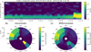 |
Fig. 1 Example case of counter-streaming ions observed by RPC-ICA inside the diamagnetic cavity on 2015 July 26. Note that the energy scale in all panels has been corrected using the lower energy cut-off method, as detailed in Section 2.3. (a) Energy-time spectrogram of ions. The magenta line indicates the total magnetic field strength. (b) The corresponding sector polar plot of ion counts, showing the instrument’s raw directional measurements. (c) The same polar plot after a directional correction has been applied using the spacecraft plasma interaction software (SPIS; Bergman et al. 2020a,b). In the polar plots (b, c), the polar axis represents the instrument’s viewing sector, while the radial axis corresponds to three re-binned energy ranges (2.5–5 eV, 5–10 eV, and 10–20 eV). The color scale indicates the ion counts normalized by the observation time for energy interval. Data from the contaminated sector 0 have been removed, and sector 13 is inactive. The blue and red arrows point toward the average directions to the comet and the Sun, respectively. |
Parameters for characterizing counter-streaming ions.
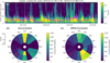 |
Fig. 2 Second example case of counter-streaming ions, observed outside the diamagnetic cavity on 2016 January 31. The energy scale for all panels has been corrected using the lower energy cut-off method. (a) Energy-time spectrogram of ions, with the total magnetic field strength overlaid as a magenta line. (b) The sector polar plot of ion counts before directional correction. (c) The sector polar plot after the SPIS-based directional correction(Bergman et al. 2020a,b). The format of the polar plots (b,c) is the same as Fig. 1: the polar axis is the instrument sector, the radial axis represents binned energy ranges (2.5–5 eV, 5–10 eV, and 10–20 eV), and the color scale shows normalized counts. Data from sector 0 have been removed, and sector 13 is inactive. The blue and red arrows point toward the average directions to the comet and the Sun, respectively. |
3.2 Statistical properties of anticometward and cometward ion flows
A statistical survey of the high-resolution data has yielded a total of 156 anticometward and 167 cometward ion flow events (Table S1). Of the anticometward events, 50 were observed inside the diamagnetic cavity and 106 outside. For the cometward flows, 67 were detected inside the cavity and 100 outside. The statistical properties of these two populations are summarized in Fig. 3.
The distributions of peak counts for both anticometward and cometward ions exhibit similar characteristics (Fig. 3a). The majority of events are concentrated in the 0–150 counts range. Furthermore, the median peak counts are comparable across all four subgroups (i.e., inside and outside the cavity for both flow directions). The center energy distributions reveal a clear distinction between the two types of flows (Fig. 3b). The distribution for cometward flows peaks in the 5–10 eV bin, whereas the anticometward flows peak at a higher energy of 10–15 eV, indicating that the latter population is, on average, more energetic. For both flow types, there is no significant difference in the energy distributions observed inside versus outside the cavity, as their respective median values are nearly identical.
Fig. 3c illustrates the distribution of the sector width. The cometward flow is typically narrow, with its width concentrated at 22.5° and 45°. No discernible difference is found between the distribution inside and outside the cavity, as both show a median width of 45°. In contrast, the anticometward flow is broader, with its width distribution peaking at 90°. A clear distinction exists based on location: the flow outside the cavity is wider (median of 90°) than that observed inside (median of 67.5°). The energy width distributions are presented in Fig. 3d. Unlike the sector width, all four subgroups exhibit similar characteristics. For all populations, both the peak and the median of the energy width distribution fall within the 10–20 eV range.
The Sun angle distribution (Fig. 3e) shows that the cometward flow events predominantly have angles less than 90°, indicating a sunward component. The anticometward flow events exhibit an antisunward component, which is more pronounced for events observed inside the cavity. This finding is consistent with observations reported by Bergman et al. (2021a). The distribution of the comet angle is shown in Fig. 3f. For the cometward flow, both the peak and the median of the distribution are found in the 30°–60° range, suggesting that this ion flow is not strictly directed toward the comet. The distribution for the anticometward flow is relatively uniform across the 90°–180° range.
Corresponding to Figs. 3 and 4 shows the statistical properties of the anticometward and cometward ion flows derived from standard-resolution data. In this dataset, we identified 403 anticometward events (136 inside, 267 outside the cavity) and 406 cometward events (136 inside, 270 outside) (Table S1). While these results are generally in agreement with the high-resolution data, two key differences exist. First, although the peak count distribution (Fig. 4a) has a similar shape to its high-resolution counterpart (Fig. 3a), its median is shifted toward higher values. This is attributed to the detection of a subset of events with very high peak counts (>1000) in the standard-resolution mode. Meanwhile, the anticometward flow exhibits a larger median peak count than the cometward flow. Second, the center energies are systematically higher, with medians in the 10–15 eV range for cometward flows and 15–20 eV for anticometward flows (Fig. 4b). This systematic shift toward higher energies may be attributed to the poorer energy resolution and less accurate sensor temperature correction in the standard-resolution mode, both of which can introduce biases in energy estimation.
 |
Fig. 3 Histograms showing the statistical distributions of six key parameters for cometward (blue) and anticometward (orange) ion flows, derived from high-resolution RPC-ICA data. The data are separated into observations inside (light shades) and outside (dark shades) the diamagnetic cavity. Each panel corresponds to a specific parameter: (a) peak counts, (b) center energy, (c) sector width, (d) energy width, (e) Sun angle, and (f) comet angle. The median value for each of the four distributions is indicated by a corresponding dashed line, as detailed in the legend in panel a. |
3.3 Statistical properties of counter-streaming ion events
To ensure that the detected flows were genuinely in opposition, a final selection criterion was applied for counter-streaming ion events: only events where the angular separation between anticometward and cometward ion flow exceeded 90° were included in the statistical analysis. As detailed in Table S2, we identified 112 counter-streaming ion events from the high-resolution data (71 in outside region and 41 inside) and 338 events from the standard-resolution data (228 outside and 110 inside). These numbers correspond to detection rates of 56% (112/199) and 76% (338/442) for the high- and standard-resolution data, respectively. The statistical distributions of these events are shown in Fig. 5.
For the high-resolution results (Figs. 5a–5c), the energy ratio distribution (Fig. 5a) shows events clustering within the first two of the three logarithmic bins in the 1–10 range, with mean values of 1.43 and 1.83 for the outside and inside populations, respectively. The comparable values indicate that the anticometward flow is consistently more energetic than the cometward flow in both regions. The count ratio distribution (Fig. 5b) is approximately normal and reveals a reversal between the two regions: outside the cavity, the anticometward flow has higher counts (mean ratio of 1.26 ± 0.19), whereas inside, its counts are lower than the cometward flow’s (mean ratio of 0.68 ± 0.15). The standard errors confirm this is a statistically significant trend, as the former ratio is clearly above unity and the latter is clearly below it. The angular separation results (Fig. 5c) are similar for both locations, peaking sharply in the 150°–180° range. The mean values are 155.28° (outside) and 150.37° (inside).
The statistical results from the standard-resolution data (Figs. 5d–5f) are broadly consistent with those from the high-resolution data. However, the count ratio reversal between the outside and inside regions is absent. The anticometward flow consistently contains higher counts than the cometward flow, although the ratio is larger for the outside region than for the inside one. Furthermore, we investigated the dependence of event properties on both cometocentric and heliocentric distances. Some trends were observed, but only within the high-resolution dataset (not shown). Events at smaller cometocentric distances tended to show larger energy ratios and smaller count ratios. Conversely, events at smaller heliocentric distances showed smaller energy ratios and larger count ratios.
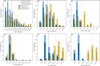 |
Fig. 4 Same as Fig. 3, but for the results derived from standard-resolution RPC-ICA data. The histograms show the statistical distributions of the six parameters for cometward (blue) and anticometward (orange) ion flows, observed inside (light shades) and outside (dark shades) the diamagnetic cavity. The median of each distribution is marked by a corresponding dashed line. |
3.4 Effects of the limited field of view
Since our analysis utilizes data from two different instrumental modes, it is crucial to discuss the implications of the reduced dimensionality of the high-resolution data, which lacks elevation information. The limited elevation coverage presents two potential challenges. First, it can lead to an underestimation of the total ion counts. Fig. 6a provides an example of this, while valid ion signals are detected within the field of view (FOV) of the high-resolution mode (outlined by the red dashed ellipse), a portion of the signal exists at other elevation angles. Another challenge is the potential for non-detection, as depicted in Fig. 6b. Here, detectable ion signals are present, but they fall entirely outside the narrow FOV of the high-resolution mode. Consequently, an event with such a distribution could be missed by the high-resolution dataset.
To quantify this effect, we statistically analyzed the fraction of ion counts detected within a FOV of 360° × 5° (emulating the high-resolution mode) relative to the full 360° × 90° FOV of the standard mode. This comparison was performed using standard-resolution data, restricted to the 0.3–82 eV/q energy range (before correction) to match the high-resolution coverage. For the anticometward sectors (4 and 5), the average fractions were found to be 20% and 25%, respectively. For the cometward sectors (14 and 15), the fractions were 36% and 27%. This shows that even though the high-resolution data uses only one elevation, it captures a significant part of the signal when event is within its FOV. However, we cannot quantify the number of events missed entirely (Fig. 6b), which likely explains the lower detection rate of counter-streaming ion events in the high-resolution (56%) compared to the standard-resolution data (76%).
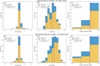 |
Fig. 5 Statistical distributions of three key parameters for counter-streaming ion events. The data are separated into observations outside (yellow) and inside (blue) the diamagnetic cavity. The top row (a–c) is derived from high-resolution data, while the bottom row (d–f) is from standard-resolution data. The panels show the energy ratio (a, d), count ratio (b, e), and angular separation (c, f). Red and blue dashed lines in each panel mark the mean values for the outside and inside cavity populations, respectively. |
4 Discussions
A key objective of this study is to characterize the velocities of the counter-streaming ion populations and their bulk flow, thereby addressing the discrepancy between previous in situ observations and the assumptions made in numerical models (Galand et al. 2016; Heritier et al. 2018). Inside and near the diamagnetic cavity, we frequently found counter-streaming ion events. As highlighted in the presentation of Case 1 (Section 3.1), which occurred inside the diamagnetic cavity, the anticometward and cometward flows are sometimes temporally separated. This temporal separation makes it uncertain whether the two flows are intermittent and sequential, or if they coexist but are observed at different times due to limited field of view of the RPC-ICA instrument. To investigate this, we manually inspected all 41 high-resolution counter-streaming events identified inside the diamagnetic cavity. We found that while the majority of events (76%) exhibit the temporal separation, a significant minority (10 events) show clear evidence of both flows being detected simultaneously.
One such event was selected for a detailed velocity analysis (11:35:04–11:36:20 UT on July 26, 2015). The results show that the anticometward and cometward flows have a velocity of 9.3 km/s. Crucially, the resulting bulk velocity of the combined population is 0.1 km/s. This single case demonstrates that two high-speed, counter-streaming populations can produce a low net bulk velocity. We confirmed this finding by analyzing the velocities for all 10 events that showed simultaneous counter-streaming ions. In these cases, the anticometward flows had velocities in the range of 8.9–11.6 km/s and the cometward flows ranged from 8.6–10.3 km/s, while the resulting bulk velocity was significantly lower, at 0.1–3 km/s. The counter-streaming phenomenon provides a mechanism to reconcile the discrepancy between high measured ion speeds by RPC-ICA (5–10 km/s, Bergman et al. 2021b) and the low bulk speeds required by kinetic models (e.g., Galand et al. 2016; Lewis et al. 2024) in the vicinity of the diamagnetic cavity. This is an issue recently highlighted as a key challenge that needs to be solved (Beth et al. 2022). The finding is also crucial for interpreting the high effective speeds (2–8 km/s) reported by RPC-LAP (Vigren et al. 2017; Odelstad et al. 2018). This is because the single-population analysis model can misinterpret two counter-streaming beams as a single, genuine high-speed flow (see Introduction).
Having established the properties of the counter-streaming flows, we now investigate the mechanism responsible for their formation. Edberg et al. (2019) has demonstrated that the solar wind convection electric field can influence cold plasma deep within the coma, even in the vicinity of the diamagnetic cavity. Therefore, a primary candidate to investigate is whether this external field (E = −v × B) is strong enough to turn the initial anticometward flow back toward the nucleus. If this mechanism was dominant, the occurrence of these events would exhibit a clear spatial asymmetry in the comet-centered solar electric (CSE) coordinate system, where the z-axis is aligned with the electric field. To test this, we mapped the locations of events outside the cavity and the pre-entry positions of events inside the cavity. The resulting distributions show no discernible asymmetry between the +Z and −Z hemispheres (not shown), suggesting that the convection electric field does not play a dominant role. This conclusion is reinforced by our energy analysis (Section 3.3, Figs. 5a and 5d), showing the anticometward flow to be, on average, comparable in energy to or even more energetic than the cometward flow, which is inconsistent with an electric field acceleration scenario.
Given the inconsistencies with the electric field model, we therefore examine an alternative mechanism based on ion gyration, a scenario first suggested for the cometary environment by Puhl-Quinn & Cravens (1995). This is similar to the situation at a magnetopause, where the larger gyro-radius of the ions allow for a magnetopause Hall electric field to arise. This electric field is a consequence of the gyro-radius of the ions, so the gyration is the primary physical mechanism. We statistically analyzed the magnetic field just outside the cavity boundary during the observed events, finding a mean and median magnitude of approximately 17 nT. The magnetic field strength corresponds to a gyro-radius of roughly 100 km for a typical cometary ion (assuming m/q = 20 amu/e and E = 5 eV). This scale is consistent with the average altitude of the observed counter-streaming events, which is approximately 150 km. The comparability of the ion gyro-radius and the characteristic scale of the cavity region strongly suggests that the cometward flow can be interpreted as the returning phase of the anticometward ions as they execute their gyration orbits in the piled-up magnetic field at the boundary.
Furthermore, this gyration model is quantitatively supported by an analysis of the pressure balance at the cavity boundary. For the high-resolution events, we calculated the mean ion dynamic pressure for both flow components. The anticometward flow exerts an outward dynamic pressure of approximately 0.2 nPa, while the returning cometward flow provides an inward pressure of about 0.05 nPa. This results in a net outward dynamic pressure from the ion population of 0.15 nPa. In opposition to this, the 17 nT magnetic field piled up just outside the boundary exerts an inward magnetic pressure of approximately 0.12 nPa. The remarkable comparability between the net outward ion pressure (0.15 nPa) and the inward magnetic pressure (0.12 nPa) suggests a state of approximate pressure equilibrium at the boundary. The magnetic gyration model thus offers a robust and self-contained explanation for the origin of the counter-streaming ion phenomenon.
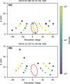 |
Fig. 6 Elevation distribution of low-energy ions from standard-resolution measurements with a corrected energy scale. Panels a and b show the distribution of ion counts in elevation-energy space for the anticometward sector (Sector 5) at two different time points. The field of view (FOV) of the high-resolution mode is outlined by the red dashed ellipse. |
5 Summary and conclusions
In this paper, we present the first statistical characterization of counter-streaming ion populations in and around the diamagnetic cavity at comet 67P/Churyumov-Gerasimenko using both high- and standard-resolution data from RPC-ICA on board Rosetta. Our analysis reveals that these events are a frequent feature in the plasma environment of this near-nucleus region, typically characterized by two oppositely directed flows. The anticometward population is generally more energetic and more intense than its cometward counterpart. The trends are consistent for populations both inside and outside the cavity. We show that the super-position of these high-speed streams produces a low net bulk velocity, potentially reconciling in situ ion measurements with results based on kinetic models. Furthermore, we propose that the cometward flow is a consequence of ion gyration within the piled-up magnetic field at the cavity boundary. This motion is not driven by the large-scale convection electric field, but is instead dictated by local forces arising from the magnetic pressure gradient and the Hall term. These findings establish a quantitative framework for this phenomenon and offer a direct observational basis to address a long-standing discrepancy between measured and modeled ion speeds near the diamagnetic cavity.
Data availability
The datasets and supplementary tables generated during this study are available in the Zenodo repository at https://zenodo.org/records/18164707.
Acknowledgements
This work was supported by the National Natural Science Foundation of China (Grant Nos. 42188101, 42025404, 42474217, 42174188, and U2541290), the National Key R&D Program of China (Grant Nos. 2022YFF0503700 and 2025YFF0512500), the Fundamental Research Funds for the Central Universities (Grant No. 242025kf0008), and the Natural Science Foundation of Hubei Province, China (Grant No. 2025AFA030). This work was also supported by the special scholarship provided through the Graduate Student Exchange Program at Wuhan University, China.
References
- Altwegg, K., Balsiger, H., & Fuselier, S. A. 2019, Annu. Rev. Astron. Astrophys., 57, 113 [Google Scholar]
- Behar, E., Lindkvist, J., Nilsson, H., et al. 2016a, A&A, 596, A42 [NASA ADS] [CrossRef] [EDP Sciences] [Google Scholar]
- Behar, E., Nilsson, H., Stenberg Wieser, G., et al. 2016b, GRL, 43, 1411 [Google Scholar]
- Bergman, S., Stenberg Wieser, G., Wieser, M., Johansson, F. L., & Eriksson, A. 2020a, JGR: Space Phys., 125, e2019JA027478 [Google Scholar]
- Bergman, S., Stenberg Wieser, G., Wieser, M., Johansson, F. L., & Eriksson, A. 2020b, JGR: Space Phys., 125, e2020JA027870 [Google Scholar]
- Bergman, S., Stenberg Wieser, G., Wieser, M., et al. 2021a, MNRAS, 507, 4900 [NASA ADS] [CrossRef] [Google Scholar]
- Bergman, S., Stenberg Wieser, G., Wieser, M., et al. 2021b, MNRAS, 503, 2733 [NASA ADS] [CrossRef] [Google Scholar]
- Beth, A., Galand, M., Wedlund, C. S., & Eriksson, A. 2022, arXiv preprint [arXiv:2211.03868] [Google Scholar]
- Biermann, L., Brosowski, B., & Schmidt, H. 1967, Sol. Phys., 1, 254 [NASA ADS] [CrossRef] [Google Scholar]
- Broiles, T. W., Burch, J. L., Clark, G., et al. 2015, A&A, 583, A21 [NASA ADS] [CrossRef] [EDP Sciences] [Google Scholar]
- Carr, C., Cupido, E., Lee, C. G., et al. 2007, SSRv, 128, 629 [Google Scholar]
- Edberg, N. J., Eriksson, A. I., Odelstad, E., et al. 2016, JGR: Space Phys., 121, 949 [Google Scholar]
- Edberg, N. J., Eriksson, A. I., Vigren, E., et al. 2019, AJ, 158, 71 [NASA ADS] [CrossRef] [Google Scholar]
- Eriksson, A. I., Boström, R., Gill, R., et al. 2007, SSRv, 128, 729 [Google Scholar]
- Galand, M., Héritier, K. L., Odelstad, E., et al. 2016, MNRAS, 462, S331 [Google Scholar]
- Glassmeier, K.-H. 2017, Phil. Trans. R. Soc. A, 375, 20160256 [CrossRef] [Google Scholar]
- Glassmeier, K. H., Boehnhardt, H., Koschny, D., Kührt, E., & Richter, I. 2007a, SSRv, 128, 1 [Google Scholar]
- Glassmeier, K. H., Richter, I., Diedrich, A., et al. 2007b, SSRv, 128, 649 [Google Scholar]
- Goetz, C., Koenders, C., Richter, I., et al. 2016a, A&A, 588, A24 [NASA ADS] [CrossRef] [EDP Sciences] [Google Scholar]
- Goetz, C., Koenders, C., Hansen, K. C., et al. 2016b, MNRAS, 462, S459 [NASA ADS] [CrossRef] [Google Scholar]
- Goetz, C., Behar, E., Beth, A., et al. 2022, SSRv, 218, 65 [Google Scholar]
- Gulkis, S., Allen, M., Von Allmen, P., et al. 2015, Science, 347, aaa0709 [NASA ADS] [CrossRef] [Google Scholar]
- Gunell, H., Goetz, C., Eriksson, A., et al. 2017, MNRAS, 469, S84 [NASA ADS] [CrossRef] [Google Scholar]
- Hajra, R., Henri, P., Vallières, X., et al. 2018, MNRAS, 475, 4140 [NASA ADS] [CrossRef] [Google Scholar]
- Henri, P., Vallières, X., Hajra, R., et al. 2017, MNRAS, 469, S372 [NASA ADS] [CrossRef] [Google Scholar]
- Heritier, K., Henri, P., Vallières, X., et al. 2017, MNRAS, 469, S118 [NASA ADS] [CrossRef] [Google Scholar]
- Heritier, K., Galand, M., Henri, P., et al. 2018, A&A, 618, A77 [NASA ADS] [CrossRef] [EDP Sciences] [Google Scholar]
- Israelevich, P. L., Ershkovich, A. I., & Ioffe, Z. M. 1992, JGR: Space Phys., 97, 17045 [Google Scholar]
- Koenders, C., Glassmeier, K. H., Richter, I., Ranocha, H., & Motschmann, U. 2015, PSS, 105, 101 [Google Scholar]
- Lamy, P., Toth, I., Jorda, L., Weaver, H., & A’Hearn, M. 1998, A&A, 335, L25 [NASA ADS] [Google Scholar]
- Lewis, Z., Beth, A., Galand, M., et al. 2024, MNRAS, 530, 66 [Google Scholar]
- Lisse, C. M., A’Hearn, M. F., Farnham, T. L., et al. 2005, SSRv, 117, 161 [Google Scholar]
- Madsen, B., Wedlund, C. S., Eriksson, A., et al. 2018, GRL, 45, 3854 [Google Scholar]
- Masunaga, K., Nilsson, H., Behar, E., et al. 2019, A&A, 630, A43 [NASA ADS] [CrossRef] [EDP Sciences] [Google Scholar]
- Nemeth, Z., Burch, J., Goetz, C., et al. 2016, MNRAS, 462, S415 [NASA ADS] [CrossRef] [Google Scholar]
- Neubauer, F., Glassmeier, K., Pohl, M., et al. 1986, Nature, 321, 352 [NASA ADS] [CrossRef] [Google Scholar]
- Neubauer, F. M. 1988, JGR: Space Phys., 93, 7272 [Google Scholar]
- Nilsson, H., Lundin, R., Lundin, K., et al. 2007, SSRv, 128, 671 [Google Scholar]
- Nilsson, H., Stenberg Wieser, G., Behar, E., et al. 2015, Science, 347, aaa0571 [NASA ADS] [CrossRef] [Google Scholar]
- Nilsson, H., Stenberg Wieser, G., Behar, E., et al. 2017, MNRAS, 469, S252 [Google Scholar]
- Odelstad, E., Stenberg Wieser, G., Wieser, M., et al. 2017, MNRAS, 469, S568 [NASA ADS] [CrossRef] [Google Scholar]
- Odelstad, E., Eriksson, A. I., Johansson, F. L., et al. 2018, JGR: Space Phys., 123, 5870 [Google Scholar]
- Ostaszewski, K., Glassmeier, K. H., Goetz, C., et al. 2021, Ann. Geophys., 39, 721 [Google Scholar]
- Puhl-Quinn, P., & Cravens, T. E. 1995, JGR: Space Phys., 100, 21631 [Google Scholar]
- Simon Wedlund, C., Alho, M., Gronoff, G., et al. 2017, A&A, 604, A73 [NASA ADS] [CrossRef] [EDP Sciences] [Google Scholar]
- Stenberg Wieser, G., Odelstad, E., Wieser, M., et al. 2017, MNRAS, 469, S522 [NASA ADS] [CrossRef] [Google Scholar]
- Szegö, K., Glassmeier, K.-H., Bingham, R., et al. 2000, SSRv, 94, 429 [Google Scholar]
- Thiebault, B., Jeanty-Ruard, B., Souquet, P., et al. 2015, IEEE Trans. Plasma Sci., 43, 2782 [Google Scholar]
- Timar, A., Nemeth, Z., Szego, K., et al. 2017, MNRAS, 469, S723 [Google Scholar]
- Trotignon, J.-G., Michau, J., Lagoutte, D., et al. 2007, SSRv, 128, 713 [Google Scholar]
- Vigren, E., & Eriksson, A. I. 2017, AJ, 153, 150 [NASA ADS] [CrossRef] [Google Scholar]
- Vigren, E., & Eriksson, A. I. 2019, MNRAS, 482, 1937 [Google Scholar]
- Vigren, E., André, M., Edberg, N. J., et al. 2017, MNRAS, 469, S142 [Google Scholar]
- Vigren, E., Edberg, N. J. T., Eriksson, A. I., et al. 2019, ApJ, 881, 6 [Google Scholar]
- Wallis, M. K. 1973, PSS, 21, 1647 [Google Scholar]
All Tables
All Figures
|
Fig. 1 Example case of counter-streaming ions observed by RPC-ICA inside the diamagnetic cavity on 2015 July 26. Note that the energy scale in all panels has been corrected using the lower energy cut-off method, as detailed in Section 2.3. (a) Energy-time spectrogram of ions. The magenta line indicates the total magnetic field strength. (b) The corresponding sector polar plot of ion counts, showing the instrument’s raw directional measurements. (c) The same polar plot after a directional correction has been applied using the spacecraft plasma interaction software (SPIS; Bergman et al. 2020a,b). In the polar plots (b, c), the polar axis represents the instrument’s viewing sector, while the radial axis corresponds to three re-binned energy ranges (2.5–5 eV, 5–10 eV, and 10–20 eV). The color scale indicates the ion counts normalized by the observation time for energy interval. Data from the contaminated sector 0 have been removed, and sector 13 is inactive. The blue and red arrows point toward the average directions to the comet and the Sun, respectively. |
| In the text | |
|
Fig. 2 Second example case of counter-streaming ions, observed outside the diamagnetic cavity on 2016 January 31. The energy scale for all panels has been corrected using the lower energy cut-off method. (a) Energy-time spectrogram of ions, with the total magnetic field strength overlaid as a magenta line. (b) The sector polar plot of ion counts before directional correction. (c) The sector polar plot after the SPIS-based directional correction(Bergman et al. 2020a,b). The format of the polar plots (b,c) is the same as Fig. 1: the polar axis is the instrument sector, the radial axis represents binned energy ranges (2.5–5 eV, 5–10 eV, and 10–20 eV), and the color scale shows normalized counts. Data from sector 0 have been removed, and sector 13 is inactive. The blue and red arrows point toward the average directions to the comet and the Sun, respectively. |
| In the text | |
|
Fig. 3 Histograms showing the statistical distributions of six key parameters for cometward (blue) and anticometward (orange) ion flows, derived from high-resolution RPC-ICA data. The data are separated into observations inside (light shades) and outside (dark shades) the diamagnetic cavity. Each panel corresponds to a specific parameter: (a) peak counts, (b) center energy, (c) sector width, (d) energy width, (e) Sun angle, and (f) comet angle. The median value for each of the four distributions is indicated by a corresponding dashed line, as detailed in the legend in panel a. |
| In the text | |
|
Fig. 4 Same as Fig. 3, but for the results derived from standard-resolution RPC-ICA data. The histograms show the statistical distributions of the six parameters for cometward (blue) and anticometward (orange) ion flows, observed inside (light shades) and outside (dark shades) the diamagnetic cavity. The median of each distribution is marked by a corresponding dashed line. |
| In the text | |
|
Fig. 5 Statistical distributions of three key parameters for counter-streaming ion events. The data are separated into observations outside (yellow) and inside (blue) the diamagnetic cavity. The top row (a–c) is derived from high-resolution data, while the bottom row (d–f) is from standard-resolution data. The panels show the energy ratio (a, d), count ratio (b, e), and angular separation (c, f). Red and blue dashed lines in each panel mark the mean values for the outside and inside cavity populations, respectively. |
| In the text | |
|
Fig. 6 Elevation distribution of low-energy ions from standard-resolution measurements with a corrected energy scale. Panels a and b show the distribution of ion counts in elevation-energy space for the anticometward sector (Sector 5) at two different time points. The field of view (FOV) of the high-resolution mode is outlined by the red dashed ellipse. |
| In the text | |
Current usage metrics show cumulative count of Article Views (full-text article views including HTML views, PDF and ePub downloads, according to the available data) and Abstracts Views on Vision4Press platform.
Data correspond to usage on the plateform after 2015. The current usage metrics is available 48-96 hours after online publication and is updated daily on week days.
Initial download of the metrics may take a while.