| Issue |
A&A
Volume 706, February 2026
|
|
|---|---|---|
| Article Number | A179 | |
| Number of page(s) | 15 | |
| Section | Stellar atmospheres | |
| DOI | https://doi.org/10.1051/0004-6361/202557717 | |
| Published online | 10 February 2026 | |
Surface image and activity-corrected orbit of the RSCVn binary HR7275
Disentangling activity tracers
1
Leibniz-Institute for Astrophysics Potsdam (AIP),
An der Sternwarte 16,
14482
Potsdam,
Germany
2
Institut für Physik und Astronomie, Universität Potsdam,
14476
Potsdam,
Germany
3
HUN-REN Research Centre for Astronomy and Earth Sciences, Konkoly Observatory,
1121
Budapest,
Hungary
4
HUN-REN CSFK, MTA Centre of Excellence,
1121
Budapest,
Hungary
★ Corresponding author: This email address is being protected from spambots. You need JavaScript enabled to view it.
Received:
16
October
2025
Accepted:
10
December
2025
Abstract
Context. Quantifying stellar parameters and magnetic activity for cool stars in double-lined spectroscopic binaries (SB2s) is not straightforward, as both stars contribute to the observed composite spectra and are likely variable. Disentangled component spectra allow a detailed analysis of the magnetic activity of the primary component.
Aims. We aim to separate the spectra of the two stellar components of the HR 7275 SB2 system. We also aim to obtain a more accurate orbital solution by correcting the observed radial velocities (RV) from activity perturbations of the spotted primary (“RV jitter”) and to derive a surface image of this component.
Methods. We obtained time-series high- and ultra-high resolution optical spectra and applied two different disentangling methods. We modeled radial velocity (RV) residuals using three-sine function fits and modeled the spectral-line profile of the primary with the Doppler imaging code iMAP. We measured magnetic fields for the primary based on least-squares deconvolved Stokes-V line profiles, and determined chromospheric emission from the line cores of CaIIH&K, CaIIIRT8542 Å, and Balmer Hα. We first applied our disentangling technique, which allowed us to determine the properties of the system more accurately before performing these analyses.
Results. The Doppler image of the primary shows two large cool spots that cover approximately 20% of the visible hemisphere, plus three smaller spots each still covering approximately 13% in size. Between May-June 2022, HR 7275a exhibited an impressive spottedness of roughly 40% of its entire surface. The RV is modulated by the rotation of the primary, with maximum amplitudes of 320 m s−1 and 650 m s−1 for two different modulation behaviors during the 250 d of our observations. This jitter is primarily caused by the varying asymmetries of the apparent disk brightness due to the cool spots. Its removal results in roughly ten times higher precision of the orbital elements. Our snapshot magnetic-field measurements reveal phase-dependent (large-scale) surface fields between +0.6±2.0 G at phase 0.1 and −15.2±2.7 G at phase 0.6, indicating a complex magnetic morphology related to the location of the photospheric spots. We also obtain a logarithmic lithium abundance of 0.58±0.1 for HR7275a, indicating considerable mixing, and 0.16−0.63+0.23 for HR7275b, which is an extremely low value.
Key words: techniques: radial velocities / stars: activity / binaries: spectroscopic / stars: chromospheres / stars: imaging / starspots
© The Authors 2026
 Open Access article, published by EDP Sciences, under the terms of the Creative Commons Attribution License (https://creativecommons.org/licenses/by/4.0), which permits unrestricted use, distribution, and reproduction in any medium, provided the original work is properly cited.
This article is published in open access under the Subscribe to Open model. This email address is being protected from spambots. You need JavaScript enabled to view it. to support open access publication.
1 Introduction
Starspots are important indicators of stellar activity and provide information on the underlying magnetic dynamo in late-type stars. These features allow us to track magnetic activity, as well as activity processes associated with different atmospheric layers, such as the photosphere and chromosphere.
Active components with huge starspots in RS CVn-type binary systems offer an excellent opportunity to monitor such activity processes. These systems were first described and studied in depth by Hall (1972), and Vogt & Penrod (1983) subsequently applied the groundbreaking Doppler imaging technique to cool stars, enabling new types of studies. The first detailed catalog of active binary stars was compiled by Strassmeier et al. (1993). Studies of RS CVn stars have yielded several fundamental results on the relationship between photospheric starspots and global magnetic activity (e.g., Strassmeier 2009). Continuing this series, our paper examines in detail the activity of another RS CVn system, HR 7275, and attempts to separate the activity signals from the precise orbital solution.
HR 7275 is a binary system with a tidally locked primary having an orbital and rotational period of ≈28 d, which various authors have confirmed using photometric methods (Fried et al. 1982; Strassmeier et al. 1989) and RV measurements (Young 1944; Eker 1989; Osten & Saar 1998; de Medeiros & Udry 1999). It is a bright-star-catalog target with a visual magnitude of 5.89 (Ducati 2002), which makes it easy to observe. The system is a double-lined spectroscopic binary (SB2) with a K2IV-III type (sub)giant primary accompanied by a warm G-type secondary. Eker (1989) determined the mass of the primary to be between 1 and 3 M⊙, while Osten & Saar (1998) gave the stellar radius as 6.2 R⊙, with a surface temperature of 4500 K. The rotational line broadening (v sin i) was measured to approximately 15 km s−1 (e.g., Osten & Saar 1998; de Medeiros & Udry 1999). Initially considered as a single-lined binary (SB1), orbital solutions were provided by Young (1944) and Eker (1989). Osten & Saar (1998) first reported an SB2 solution, which was subsequently revised shortly afterwards by de Medeiros & Udry (1999). Based on the solutions by Eker (1989), Osten & Saar (1998) found that the secondary star has a mass of 0.9-1.1 M⊙ and a surface temperature of 5500K.
In the case of an SB2 system such as HR 7275, spectral disentangling is the first step before determining precise stellar parameters. Several technical approaches exist for this purpose (e.g. Hensberge et al. 2008; Weber & Strassmeier 2011; Sablowski et al. 2019). Osten & Saar (1998) used a grid of template stars to fit the components of the HR 7275 system within the combined spectrum. Weber & Strassmeier (2011) used a similar technique, but with a synthetic spectral grid, for Capella (α Aur), a system of two G giants. Folsom et al. (2010) developed an iterative technique called direct spectral decomposition and successfully applied it to the eclipsing binary AR Aur. Another iterative method, developed by Kriskovics et al. (2013), combined spectral disentangling with Doppler imaging to recover the surface temperature maps of both components of the SB2 pre-main-sequence system V824 Ara.
TiO lines are often used to estimate starspot coverage and temperatures (Neff et al. 1995). Using this method, O’Neal et al. (1996) studied five active and evolved stars, including HR 7275 and determined a spot temperature of 3600 K with a filling factor of 31%. However, starspots, in addition to tracing activity-related magnetic phenomena, can degrade the accuracy of spectroscopic RV measurements. Moreover, Strassmeier et al. (2024) show that spots not only interfere with RV measurements, but also, in the case of relatively near objects, such as the spotted giant XX Tri, create significant rotation-induced stellar photocenter variations, which impose limitations, e.g., for astrometric-based exoplanet searches. Thus, these effects must be taken into account for precise orbital calculations, especially when detecting a third companion, such as an exoplanet or a third body in a binary system. Saar & Donahue (1997) showed that starspots could produce RV perturbations of up to 200 m s−1, while Hatzes (2002) demonstrated that these perturbations were correlated with v sin i (up to 13 km s−1 in their simulations) and the spot-filling factor. Desort et al. (2007) also showed how a single spot on a Sun-like star affected line bisector variations. While their simulations included only a single spot, Boisse et al. (2011) used a more sophisticated two-spot model, with which they also performed inclination tests. Most recently, Zhao & Dumusque (2023) developed SOAP-GPU, a code that allows the user to efficiently model stellar activity at the spectral level, even for complex activity region configurations. Finally, based on ultra-high-resolution spectroscopic data of the RS CVn system λ And, we demonstrated the effects of starspots on RV measurements based on real observations, which are subsequently considered when correcting the orbital elements of the binary (Adebali et al. 2025).
The structure of this paper is as follows. In Sect. 2, we present our observations and the data reduction process. In Sect. 3, we provide a detailed description of our spectral disentangling routines, along with the RV calculations and the starspot correction required to improve the accuracy of the orbital solution. We present the Doppler imaging process in Sect. 4, while the investigation of chromospheric activity is covered in Sect. 5, together with magnetic field measurements and lithium abundance analyses. We summarize and conclude our findings in Sect. 6.
2 Observations and data reduction
2.1 SES/STELLA
Using the 1.2 m STELLar Activity (STELLA) robotic telescope (Strassmeier et al. 2004) with the STELLA Echelle Spectrograph (SES), we obtained a total of 148 high-resolution (R=55 000) spectra with a high signal-to-noise ratio (S/N). Data were autonomously collected with STELLA once per clear night during the 2021 and 2022 observing seasons. The SES is a fixed-format echelle spectrograph equipped with an e2v 4k×4k CCD featuring 15 μm pixels and a fiber-fed structure. The spectral resolution, with a sampling of three pixels per resolution element, is achieved through a two-slice image slicer and a 67 μm octagonal fiber that projects to 3.8 arc seconds on the sky. The wavelength coverage ranges from 3900 to 8800 A. This corresponds to an effective resolution of 110 mÅ, or 5.5 kms−1 at 6000 Å. Typical observations used an integration time of 280 s, yielding an average S/N of about 400 per pixel. Although thermally housed, the spectrograph is not pressure stabilized, resulting in a radial-velocity stability of at best 30 ms−1 (Strassmeier et al. 2023).
The SES data reduction pipeline is based on IRAF and is described in detail in Weber et al. (2016). The CCD images were corrected for bad pixels and cosmic-ray impacts. Bias levels were removed by subtracting the average overscan from each image, followed by subtracting the mean of the (already overscan-subtracted) master bias frame. The target spectra were flattened by dividing by a nightly master flat. After removal of the scattered light, the 1D spectra were extracted using the standard IRAF optimal extraction routine. The blaze function was then removed from the target spectra, followed by wavelength calibration using consecutively recorded Th-Ar spectra. Finally, the extracted spectral orders were continuum normalized by dividing with a flux-normalized synthetic spectrum.
2.2 PEPSI/VATT and PEPSI-POL/LBT
The 1.8-m Vatican Advanced Technology Telescope (VATT) was used in combination with the Potsdam Echelle Polarimetric and Spectroscopic Instrument (PEPSI) at the Large Binocular Telescope (LBT; Strassmeier et al. 2015). The PEPSI instrument is a stabilized and fiber-fed echelle spectrograph, with two arms (red and blue), each equipped with three cross dispersers (CDs). For HR7275, we used only three of the six CDs (CD III+CD V and CD III+CD VI). The wavelength regions covered were 48005440 Å (CDIII) and 6278-9067 Å (CDV and CDVI). In its VATT mode, the spectrograph provides a two-pixel resolution of R=250 000. The instrument is located in the basement of the LBT with a fiber connection of 450 m from the VATT. The VATT was operated manually each night from UT May 10, 2022 to June 14, 2022, and thus covered one full rotation of the target star sampled by 28 spectra.
We obtained high-resolution Stokes IQUV spectra of HR 7275 on three separate nights, July 7, October 15, and October 22, 2024, using the PEPSI polarimeter (PEPSI-POL) on the 11.8 m LBT. We carried out circular polarization measurements with a super-achromatic quarter-wave retarder paired with a Foster prism serving as the polarizing beam-splitter. Observations were taken at two retarder positions, offset by 90o, and processed using the differential method outlined by Ilyin (2012), yielding the Stokes I and V spectra discussed in Sect. 5. These polarimetric observations achieved a resolving power of 130 000 (2-pixel sampling), with a combined S/N of up to 3700:1 per pixel in the red wavelengths of the Stokes-I spectra, based on six sub-exposures per dataset.
Data obtained with VATT and LBT PEPSI were reduced using the Spectroscopic Data Systems for PEPSI (SDS4PEPSI) package, which is based on Ilyin (2000) and is further detailed by Strassmeier et al. (2018, 2015). The reduction procedure comprises several image-processing steps, beginning with bias subtraction and variance estimation of the raw frames, followed by super-master flat-fielding to correct CCD spatial noise and subtraction of scattered light. The pipeline then identifies the echelle orders and computes the wavelength solution from ThAr calibration images. Optimal extraction of the image slicers is then performed, together with the removal of cosmic spikes. The extracted spectra are normalized using the master flat-field spectrum to eliminate both CCD fringes and the blaze function. Finally, a global 2D continuum fit is applied and all orders are rectified into a 1D spectrum.
3 Data analysis
The observed spectra were analyzed using different techniques. First, we disentangled the two components to obtain a clearer picture of the activity behavior of the primary star. Then, we applied two different orbital solutions, both before and after the activity correction of the RV data points. The details of those processes are as follows.
3.1 Spectral disentangling with DISTRACT
Because HR 7275 is an SB2 system, we determined the orbit of the secondary component by disentangling the spectra using the code we developed for this purpose. The DIsentangler for STellaR ACTivity (DISTRACT) code comprises two techniques for the two datasets with different spectral resolutions. For the lowerresolution STELLA data, we applied a 2D cross-correlation technique to compute the SB2 solution. The higher-resolution PEPSI spectra were disentangled using a median-subtraction technique. While both approaches ultimately produced a spot-corrected orbital solution, the use of both techniques allowed a more accurate determination of the system’s orbit, activity diagnostics, and the determination of stellar parameters of both stars in the system.
3.1.1 Two-dimensional cross-correlation
Given the spectral resolution of the STELLA spectra, tracking the secondary star is possible using a model spectrum fitted to the observed spectra. For this purpose, we used two MARCS template spectra with Teff=4500 K, log g=3.0 and [Fe/H]=−0.5 for the primary star and 5500 K, 4.0, and 0.0 for the secondary (Gustafsson et al. 2008). We convolved the template spectra, setting v sin i to 15kms−1 for the primary and 3kms−1 for the secondary. We then applied a set of RV shifts between the templates to calculate the 2D cross-correlation functions (2D-CCFs) for each velocity shift. The locations of the peak values in the 1D projections of the 2D-CCF power spectrum indicate the different RV values of the two stars. These values are marked with blue circles along the orbital phase in Fig. 1 (filled for the primary star and open for the secondary). Further details of this technique can be found in Weber & Strassmeier (2011).
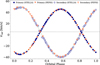 |
Fig. 1 Phase-folded radial velocities of both stars in the system. Circles indicate STELLA observations; triangles show PEPSI observations. The green lines (solid and dashed) represent the orbital fit, while the dashed black line marks the center-of-mass velocity. |
3.1.2 Median subtraction
The uniquely high resolution of the PEPSI spectra allows for easy detection of the secondary star. To this end, we arranged the observed spectra according to the orbital phase and compiled the dynamic spectrum between 4800 and 5400 Å, shown in the lower panel of Fig. 2. In the rest frame of the primary star, the lines of the secondary star clearly shift according to the orbital phase. To separate the spectra of the two stars, we first prepared equally sampled time-series composite spectra in the rest frame of the primary.
We then determined the median value of all observations for each wavelength value (i.e., the medians of the columns in the lower panel of Fig. 2). This resulted in a single 1D median composite spectrum. We then subtracted the median composite spectrum from each observed composite spectrum. This yielded the secondary spectrum for each observation time, taking into account the intrinsic variability of the primary star’s activity. After orbital velocity corrections, we averaged these median-subtracted spectra to obtain the mean spectrum of the secondary star. This spectrum is shown in Fig. B.1 together with a template spectrum of the secondary star. This technique for disentangling the stellar spectra has the advantage of being model-independent and preserves the line-depth ratio of the stars.
3.2 Further RV analysis
During the disentangling process, we obtained the RV values of both stars. To track the primary star’s activity changes on the RV curve, we performed the following steps. From all observed spectra, we subtracted the mean secondary spectrum, shifted by the corresponding RV values for each observation time. This yielded the spectrum of the primary star for each observing day. We calculated the RV values of HR 7275a by cross-correlating these spectra with a MARCS template spectrum, assuming Teff=4500 K, log g=3.0, [Fe/H]=−0.5, and v sin i broadening of 16 km s−1.
At this stage, the zero-point offset between the STELLA-SES and PEPSI instruments must be taken into account. Strassmeier et al. (2023) found the SES-minus-PEPSI grand mean RV difference to be −395±209ms−1. Adebali et al. (2025) found this difference to be −180ms−1 for the RS CVn system λ And. In this study, we obtain the same difference of −180ms−1 for HR 7275 by calculating the difference of the mean values for this observing window, and used it to correct the SES RV values to match PEPSI. The PEPSI data for λ And and HR 7275 were obtained during the same nights within a short time interval and are expected to be practically equal. The uncertainty, estimated from the minimization of the rms of the orbital SB1 fit, is at most 137ms−1.
Because STELLA is a robotic telescope, observations were made nightly according to the scheduled times, although some spectra had low S/N as a result of unfavorable weather conditions. Therefore, to eliminate outliers in the RV dataset, a 3σ clipping was applied, resulting in the removal of 14 low-S/N spectra. The resulting high-quality RV data were used in the subsequent analysis.
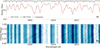 |
Fig. 2 Spectral disentangling by median subtraction. Panel a: the mean spectrum of the secondary star is shown as a black line (top). The composite spectrum (blue) and the primary star spectrum (red) are plotted with a vertical shift of 0.15 at orbital phase 0.82. Panel b: time series composite spectra phase-folded with the orbital period. |
3.3 Spot correction
A major challenge for stars with large cool spots is determining the RV jitter caused by these dark features, which distort the observed spectra. Depending on the size of the starspot and its location on the stellar disk, the spot blocks the incident light beam and shifts the core of the spectral line. If the spot is located on the approaching half of the stellar disk, it blocks the light in such a way that a net redshift is observed; if it is located on the receding half, the lack of light causes a net blueshift (see Menuier 2023). These modulations produce a sinusoidal shape, which Saar & Donahue (1997) modeled to quantify their effect on the RV curve. More complex models and observations have also been performed to obtain precise RV observations for detecting exoplanets or long-term activity modulations on stellar surfaces (e.g., Boisse et al. 2011; Zhao & Dumusque 2023; Adebali et al. 2025).
HR 7275a is very active, not only compared to the Sun, but also relative to similar active stars, such as λ And, which we recently studied (Adebali et al. 2025). Because of the large starspots, spot-related modulations in its RV curve are easier to track than for stars with smaller spots. To track the effect of spots, we obtained an SB1 orbital solution for the primary using approximately nine orbital revolutions of RV data, as shown in Fig. 3. The resulting observed-minus-calculated (O - C) residuals are presented in the bottom panel of the figure. The RV variations depicted in the O - C curve exhibit a complex modulation over a timescale of ≈250 d. Two trends are evident, separated by an observing gap of approximately 60 days (two stellar rotations): an epoch of lower jitter followed by an epoch with twice the jitter. To model these two amplitudes, we fitted three-sine functions with a small period shift, which is typically caused by residual spot migration in latitude due to differential surface rotation. This was introduced as a time-dependent period shift with a calculated maximum of approximately two days during our observation window. The first global behavior is indicated in the bottom panel of Fig. 3 by a thick gray line between BJD 2 459 640-828. During this observing window, we calculated an RV modulation of up to 320 m s−1, with a stellar rotation period of 28.58±1.3 d (e.g., Fried et al. 1982; Strassmeier et al. 1989). The periodicity clearly indicates a global cause of the activity-induced RV variability. The second behavior between BJD 2 459 828-900 is indicated in the bottom panel of Fig. 3 by a thick orange line and was modeled in the same way. Although the data points are more sparsely distributed, we still detect the same period of 28.62 ± 1.9 d but with a much higher RV amplitude of 650 m s−1 for the second global behavior. Both calculations were performed using the minimum χ2 approach of the scipy package (Virtanen et al. 2020). To remove these spot effects from the final RV model, we subtracted these fitted residual functions from the observed RV data.
Figure 4 shows the Lomb-Scargle periodogram of the fitted RV residuals, indicating the strongest peak at exactly half the rotation period. A second peak occurs at one-third of the stellar rotation period. This phenomenon is not unusual for stars with multiple spot configurations (see, e.g., Boisse et al. 2011; Adebali et al. 2025) and is observed not only in RV residuals but also in photometric modulations (e.g., Kővári et al. 2013).
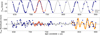 |
Fig. 3 Radial velocities of HR 7275a from VATT+PEPSI and STELLA+SES. Top panel : SB1 orbital fit is shown as a black line along with the data. Observations from STELLA+SES are indicated with dark blue circles and VATT+PEPSI observations are shown as red triangles. Bottom panel: RV residuals after subtracting predicted orbital velocities. The RV jitter appears multi-peaked per rotation. The thick gray and orange lines highlight two different rotational-modulation models. |
Orbital elements for HR 7275.
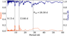 |
Fig. 4 Lomb-Scargle periodogram (red) of RV residuals from Fig. 3. The strongest peak occurs at half the stellar rotation period, while one-third of the rotation appears prominently as the second strongest peak. Phase dispersion minimization (PDM) is shown in blue, with its strongest peak at 27.2 days. |
3.4 Spot-corrected orbital solutions
We used both SB1 and SB2 configurations for our orbital solutions. For the eccentric anomaly in both configurations, we followed the method published by Danby & Burkardt (1983). For the Keplerian orbit fitting, we used the Python-scipy implementation of a least-square algorithm. The procedure was as follows. We first determined an SB1 orbit using all available data from Young (1944), Eker (1989) and Osten & Saar (1998), spanning over 80 years. From this calculation, we retained only the orbital period and subsequently fixed this value. We then determined an SB2 solution, followed by a spot-corrected SB1 orbit for the primary. Table 1 lists the final spot-corrected solutions, along with the best solutions taken from the literature. HR 7275 exhibits a stable, synchronized, and nearly circular orbital configuration. Although the secondary star may also have spots, their effect is negligible compared to that of the K2IV-III primary, due to the difference in brightness and the star’s low v sin i of ≈ 1-2 km s−1. Therefore, we did not calculate a spot correction for the secondary.
Our initial spot-uncorrected SB2 solution already provided significantly better fits than the most recent orbital calculation by de Medeiros & Udry (1999). After spot correction, the error for an observation of unit weight decreased further from 0.51 km s−1 to 0.49 km s−1 for the SB2 solution, and from 0.22 to 0.14 for the SB1 solution. On average, the errors of the orbital elements decreased by almost a factor ten compared to de Medeiros & Udry (1999), who favored a marginal non-circular orbit with a low eccentricity of 0.005 ±0.001. Although the surface spots of HR 7275a change slowly with each rotation, the spot correction still allows an orbital solution for the primary alone. This solution is more than twice as accurate as the SB2 solution due to the more precise RV measurements for the primary relative to the faint secondary and is listed in Table 1.
4 Doppler imaging
4.1 Data input and code summary
We reconstructed the surface map of HR 7275a using the iMAP code (Carroll et al. 2012), employing a multi-line inversion approach based on an average spectral line constructed from more than 500 individual lines with line depths exceeding 60% of the continuum. The rotational line broadening of 15.4km s−1 makes HR 7275a a difficult but feasible Doppler imaging (DI) target. Atomic data for the multi-line inversion were drawn from the Vienna Atomic Line Database (VALD-3; Ryabchikova et al. 2015), covering the 4800-5400 Å wavelength range of our PEPSI CD III spectra. We chose the 4800-5400 Å range for DI because CD III exposures were available for every observing night, providing the best phase coverage compared to red CDs. We computed the (pseudo) average spectral line using a singular value decomposition (SVD) algorithm, determining the dimensionality (rank) of the signal subspace via a bootstrappermutation test (see Carroll et al. 2012, for details). We obtained noise estimates in a similar way from the bootstrap procedure. This methodology results in weighted mean line profiles with typical S/N of approximately 20000 per pixel, substantially higher than the ≃400-900 S/N achieved for the individual spectra.
The high resolving power of the PEPSI spectra (R — 250 000; corresponding to 1.2 km s−1 or 0.024 Å at 6000 Å), combined with the mean full width of the spectral lines at continuum level (2 λ/c v sin i — 0.6 Å), provided 25 resolution elements across the projected stellar disk. Following the simulations by Piskunov & Wehlau (1990), which suggest that at least five resolution elements are required for successful DI, the PEPSI data were properly dimensioned for surface reconstruction. In contrast, the lower resolving power of the STELLA+SES spectra (R=55 000) renders them a borderline case for DI.
The computation of local line profiles within iMAP involves solving the radiative transfer equation for each surface pixel across 72 depth points, using a grid of tabulated Kurucz ATLAS-9 model atmospheres (Kurucz 1993; Castelli & Kurucz 2003). The local line profiles were calculated assuming 1D geometry and local thermodynamic equilibrium (LTE). The atmospheric grid spanned effective temperatures from 3500 K to 8000 K in increments of 250 K, interpolated to match the stellar surface gravity, metallicity, and microturbulence parameters obtained from global spectrum synthesis. We divided the stellar surface into 5°×5° elements, corresponding to a grid of 72×36 pixels, for a total of 2592 surface segments. We adopted a stellar inclination of 56°, calculated from stellar parameters obtained from the literature and Parameters-from-SES (ParSES) results. We reconstructed the surface using an iteratively regularized Landweber method, implementing a fixed-point iteration scheme designed to minimize the sum of the squared residuals. The method uses the noise level of the dataset as a fixed-point and stops the iteration when the sum of the squared residuals reaches the noise limit. In other words, this iteration technique works in the opposite direction to methods such as Tikhonov or maximum entropy methods, where the noise level is incorporated as an additional term in the χ2 during the iteration (see Carroll et al. 2012, and references therein). Our final image was achieved with a χ2 of 0.005.
4.2 Adopted stellar parameters
As we disentangled both spectra, we obtained stellar parameters for both stars. For the photospheric parameters, we compared the SES spectra with synthetic templates. Our code ParSES (Allende Prieto 2004; Jovanovic et al. 2013) is a software package that employs a grid of precomputed model spectra generated with Turbospectrum (Plez 2012) and a line list obtained from VALD-3 Ryabchikova et al. (2015). The ParSES code selects the best fit to the observed spectra based on the minimum distance method with a nonlinear simplex optimization (Allende Prieto et al. 2006). We applied this procedure to 122 STELLA spectra observed over a time span of 260 days for the primary star. The ParSES code returned five stellar parameters: effective temperature Teff, projected rotational velocity v sin i, microturbulence ξt, gravity log g, and metallicity [M/H]. The derived values are: Teff=4480±70K, vsini =15.4±1.2kms−1, ξt=2.0±0.2kms−1, logg=2.8±0.2, and [M/H]=−0.19±0.10. The uncertainties correspond to the 1σ rms values from the 122 individual spectra. Our v sin i and ξt values agree with those previously computed by Osten & Saar (1998). Strassmeier et al. (1989) showed that the visual magnitude of HR 7275 varies with an amplitude of 0.002-0.2 mag. This variation affects the determination of Teff by —230 K. For the time span of our observations, these values are consistent with those calculated by O’Neal et al. (1996) and Osten & Saar (1998). Using the parallax from Gaia Collaboration (2023), we calculate a luminosity of 30.6±2.8 L⊙ based on V=5.893 mag, Av = 0, and a bolometric correction of −0.48 from Popper (1980). The Stefan-Boltzmann law then suggests a probable radius of 9.2R⊙ for the primary component. Combining the ParSES value for log g with this radius, we derive a likely mass of 1.93 ±0.45 M⊙ for the primary star. Using this formal mass, we estimate that the most-likely inclination of the orbital plane is ≈52°.
Before the iterative Doppler-imaging process, we ran several test solutions with different inclinations of the rotational axis of the primary, i. Solutions in five-degree steps from i = 20° to i = 70°, with fixed v sin i provide a best fit at i = 50°, based on the minimum χ2, with an equally likely range of approximately ±7°. This value agrees closely with the inclination derived above. Assuming that the rotational axis of the primary is perpendicular to the orbital plane, we can also use this inclination for the orbital elements to obtain real masses.
Because our Doppler imaging assumes a perfectly spherical star, we estimated the oblateness of the primary due to tidal forces or rapid rotation based on the orbital parameters in Table 1, the stellar parameters in Table 2, and a range of Love numbers following Leconte et al. (2011). The expected polar-to-point radius range never exceeded 0.38-1.4%. This verifies that our spherical-shape assumption is reasonable, as the star experiences no significant elongation.
We also calculated stellar parameters for the secondary star using ParSES. For this, we employed a disentangled PEPSI spectrum of the secondary star (Fig. B.1) obtained with the mediansubtraction method explained above. We obtained the stellar parameters for the secondary star as follows: Teff=5530±116K, v sin i =1.4±0.3kms−1, ξt=0.8±0.2kms−1, log g=4.0±0.2, and [M/H]=−0.18±0.11. Table 2 summarizes the stellar parameters for both stars. Using the SB2 orbital solution, we find that the secondary mass is 1.75±0.48 M⊙.
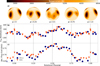 |
Fig. 5 Panel a: Doppler image of HR 7275a. The rotational phases are indicated via phase φ with a sampling of 0.25. Panel b: contemporaneous RV modulation due to spots. Panel c: relative flux modulation of CaIIIRT8542 Å simultaneous to the DI. Dark blue dots represent the STELLA dataset and red triangles indicate the PEPSI observations. |
Stellar parameters obtained in this work.
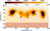 |
Fig. 6 Mercator map of the spotted surface of HR 7275a. |
4.3 Doppler imaging results
Figure 5 shows the spot configuration of HR 7275a during our May-June 2022 observations. The image was obtained from a single rotation of the star and is presented in orthographic projection with four equally spaced rotational phases. Figure 6 shows the same image in a pseudo-Mercator projection for a more global view of the stellar surface. We did not reconstruct a cool (dark) polar spot. Instead, we observe a weakly warmer (bright) region approximately 100 K hotter than the quiet surface of HR 7275a. This feature is likely unreal as the expected temperature uncertainty in the reconstruction is about 100 K, mostly due to the comparably low rotational line broadening and residual uncertainties from our LTE assumption.
In total, we observed five cool spots that appear separated in longitude by 60° on average. The spot locations, temperature differences, and surface coverages relative to the visible stellar surface are given in Table 3. Among these five spots, three (denoted A, B, and E) possibly exhibit solar-like umbral and penumbral structures, with an umbral spot ∆T ≃ 1000 K below the quiet stellar photosphere. Spots C and D appear significantly warmer than spots A, B, and E, with ∆T ≃ 500 K relative to the photosphere. Both spots lie close together in the same surface region near the quadrature phase ≈0.6, that is, in the trailing hemisphere 90° behind the binary apsidal line.
Spots on HR7275a in May–June 2022.
5 Magnetic activity and lithium abundance
5.1 Line-core emissions of Ca II H&K, Hα, and Ca II IRT8542Å
in this work, we used four chromospheric activity indicators: CaIIH&K, Hα, and one of the infrared triplet lines, CaIIIRT (8542 Å). As shown in Fig. B.3, these diagnostics cover a total of six rotations; four consecutive stellar rotations fall within the BJD 2 459 653-766 window, while two additional consecutive rotations occur between 2 459 824 and 2 459 882.
We measured the relative flux within a 1 Å bandwidth centered on the line cores at 3968.5 Å and 3933.7 Å for CaIIH&K, 8542.1 Å for CaIIIRT, and 6562.8Å for Hα. For the Ca IIIRT and Hα lines, we used spectra from both STELLA and PEPSI, whereas we performed the Ca II H&K analysis exclusively with STELLA data because the PEPSI+VATT spectra did not cover the bluest wavelength regions owing to the long fiber. We based the surface temperature calculations on ParSES, as explained in Sect. 4.2. We computed the fluxes for Hα and CaIIIRT after disentangling the spectra in the corresponding wavelength regions. Figure 7 shows the resulting secondary-star spectra for Hα and Ca II IRT regions. Because our disentangling processes failed for the Ca II H&Kregion, mainly owing to the low S/N and the intrinsic variability of the primary, we calculated the Ca II H&K line fluxes from the composite spectra. The relative contribution of the secondary must be rather small in this wavelength region. This is because the secondary’s v sin i component is very small, so it is not expected to be very active. Additionally, owing to the nature of the RS CVn systems, the strong line emission of the primary star is expected to dilute signatures from the companion.
Before converting to absolute flux, we matched the continuum settings of the STELLA spectra with those of the PEPSI spectra because of the latter’s superior quality and data reduction (Järvinen & Strassmeier 2025). Intrinsic flux-variability amplitudes were determined using three sinusoidal fits for each of the four consecutive stellar rotations. Table 4 lists the average amplitude of the chromospheric flux variability and its rms values relative to these fits.
The chromospheric activity of HR 7275 was strongly modulated with either the rotational period (≃28 d) or half that period (≃14d), depending on its single- or double-humped profile (see Table A.3). Figure B.3 shows that the maximum amplitude change is about 35% for CaIIH&K and CaIIIRT 8542Å, and 40% for Hα. The peak-amplitude locations of these emissions appear at shifts of approximately 0.1 phase per rotation, although the overall activity modulation appears to be stable during the first four rotations. During the third of the covered six full stellar rotations, corresponding to the epoch of our photospheric Doppler imaging, we observe a complex double-peaked flux distribution with the strongest peak at approximately phase 0.55 (Fig. 5c), which coincides with the central-meridian passage of the two weakest (warmest) spots, D and C. The secondary peak, about half as strong, appears around phase 0.15 and coincides with the central-meridian passage of the large spot, A. Both peaks appear similarly in the other three chromospheric tracers. The main peak at phase 0.55 is particularly prominent in Hα, indicating a facular origin, or at least a contribution by solar analogy.
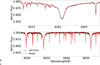 |
Fig. 7 Disentangled spectrum of HR7275b near Hα (upper panel) and the Ca II IRT region (lower panel). The observed spectrum is shown as a black line, and the model is indicated by a dashed red line. |
Logarithmic absolute emission-line fluxes (in erg cm−2 s−1) for HR 7275.
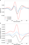 |
Fig. 8 Stokes V magnetic field measurements for HR 7275 from 2024. Panel a: LSD line profiles from PEPSI, in units of normalized intensity. Panel b: integrated Stokes-V profiles, in units of Gauss. |
5.2 Magnetic field measurements
We obtained magnetic field measurements from three PEPSI Stokes-V spectra in 2024. The spectra cover the wavelength range from 4800 Å to 5441 Å and were converted to least squares deconvolution (LSD; e.g. Donati et al. 1997) line profiles using the most recent line list from VALD-3 (Ryabchikova et al. 2015). For the magnetic field measurement, we implemented the prescription from Kochukhov et al. (2010) based on the method of Solanki & Stenflo (1984). Fig. 8a shows the three LSD profiles.
The disk-integrated longitudinal magnetic field measures −15.2±2.7 G for the July 2024 spectrum. For the two October 2024 observations, taken seven days apart, we obtain divergent results of +0.6±2.0G and −14.0±2.6G (see Table 5). Although these three measurements do not allow us to determine the global morphology of the field, they indicate the presence and phase dominance of even and odd polarities coexisting over short phase intervals on the surface.
Magnetic field measurements for HR 7275.
5.3 Lithium abundance
To estimate the internal mixing of the stars, we determined the logarithmic lithium abundance, A(Li), of the primary star and attempted to measure it for the secondary star. After disentangling the spectra in the 6300-7400 Å region using the median-subtraction technique described in Sect. 3.1.2, we constructed median spectra from all 26 PEPSI spectra of the primary and secondary stars. These two steps, disentangling and phase averaging, identified the spectrum of each star individually and removed the telluric contamination, enabling a more accurate calculation for the internal mixing of the stars. The resulting single spectrum is of high quality, with a median S/N per pixel of 300:1 for the primary and 99:1 for the secondary.
As a next step, we employed the line-synthesis program Turbospectrum (Plez 2012) together with the TurboMPfit fitting routine (Steffen et al. 2015) and the line list from Meléndez et al. (2012). We obtained multiple fits for the primary star, testing the inclusion and exclusion of TiO lines, fixed and adapted continuum level, line shifts, and macroturbulence broadening. Interestingly, the impact of the TiO molecular lines is moderate, despite the low Teff of 4480 K. This is likely due to the lower particle densities in the line-formation regions of this giant star at log g=2.8. Figure 9a shows the best fit, with an abundance of 0.58±0.1, with or without TiO blends. The relatively large error of ±0.1 dex, is dominated by the ±70 K uncertainty in the ParSES-based Teff. The internal fit quality of all Turbospectrum runs remained around or below 0.01 dex, a factor ten lower, because the fit was much more sensitive to the overall photospheric effective temperature. Furthermore, the TiO lines do not significantly affect the fit; both versions yield abundances differing by less than 1%. Although HR 7275a has spots 1000 K cooler than the surrounding photosphere, which should favor local TiO line formation, the effective temperature of the star is too high for these lines to be detectable (Strassmeier & Steffen 2022). Adebali et al. (2025) reported similar results for λ And, which is only about 100 K hotter than HR 7275a.
We applied a similar procedure to the secondary spectrum, but we adopted the continuum at 6708 Å as a free parameter from the start, and fixed line shift and broadening. This left only the continuum and the Li abundance as free parameters, due to the low S/N. We obtained fits for three effective temperatures, ±115 K around the nominal Teff of 5530 K, and three relative metallicities 0: −0.1, and −0.2. The best fit was obtained for Teff=5530K and [Fe/H]=−0.1, yielding A(Li)=0.16dex, as shown in Fig. 9b. Although its internal error is negligible, we estimated a real error from the ±115-K temperature range and ±0.1 dex metallicity variation, indicating a marginal lithium detection of A(Li)=+0.16 . The final lithium abundance for the primary is robust, A(Li)=0.58±0.1 dex, indicating significant mixing, as expected for an evolved star. We could not determine the 6Li/7Li isotopic ratio from the highly broadened spectrum, so we fixed it at 0.0. The lithium abundance of the secondary appears extremely low. For comparison, the single benchmark star 70 Vir (also classified as G4 V-IV) has A(Li)=1.12, roughly ten times higher than for HR7275b.
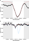 |
Fig. 9 Lithium abundance analysis. Panel a: median spectrum of HR 7275a (black dots) and Turbospectrum fit (dashed red line). The gray shaded areas indicate the regions outside the fitting range (white). Panel b: same as panel a, but for HR 7275b. The dashed blue line shows a PEPSI spectrum of 70 Vir. |
6 Summary and conclusions
We used various techniques to understand the activity behavior of the primary star in the HR 7275 system. We developed a python tool, DISTRACT, which employs two methods to isolate the spectra of two stars. This approach enabled us to quantify the following activity indicators for HR 7275a.
The average RV jitter of HR 7275a is comparable to that observed for the highly asynchronous primary star in the λ And system (Adebali et al. 2025). The RV contribution from HR 7275a spots exhibit two distinct global modulation patterns. The first pattern produces up to 320 m s−1 of RV jitter, while the second global modulation pattern peaks at 650 m s−1. Our global fits for these modulations provide an estimate of the general activity behavior of the star. However, the activity modulation differs from one rotation to another. Between BJD2 459 6402 459 828, we observed four consecutive rotations with sufficient sampling. During the first rotation, the RV modulation reaches up to 600ms−1 but decreases to 200ms−1 in the next two rotations, resulting in an average of 320 m s−1 across all four rotations. After BJD2 459 828, we obtained two addition but less well-sampled rotations. Both show a larger spread in RV jitter and a higher average of 650ms−1. We attribute this change to disk asymmetry caused by the relative positions of the spots and the stellar limb. This may be a feature that separates HR 7275a from its asynchronously rotating RSCVn cousin λ And, which shows stable spot coverage and RV jitter over 522 d (almost ten stellar rotations). Additionally, the presence of three relatively large spots, each occupying almost 10% of the surface of HR 7275a, indicates a more intense dynamo process than in λ And. We conclude that synchronized rotation does not necessarily favor more stable magnetic structures or more stable stellar magnetic activity.
We also observed this aspect in the chromospheric emissions. Figure B.3 shows that the activity peaks appear at different relative flux values. For CaIIH&K and CaIIIRT8542 emissions, the highest activity appears during the second stellar rotation. In contrast, Hα emission flux peaks during the third rotation, where we also construct the Doppler image of the primary star. This indicates that the emission fluxes in the Hα regime do not exactly follow the behavior of the Ca II IRT and CaIIH&Kfluxes. Considering the formation heights of these emission lines, we conclude that the more intense dynamo behavior affects different chromospheres to varying degrees.
Characterizing the activity jitter on RVs and confirming these effects with Doppler imaging provides a broader understanding of how starspot structures affect chromospheric emission. Figure 5 shows that the warmer spots produce stronger Ca II H&Kemission. We interpret this as a faculae-dominated region heating the upper atmosphere more than the cooler spots on HR 7275a. This effect is also observable in the Sun, where magnetic fields serve as the main heating mechanism in the chromosphere. The dominant spots C and D also appear closer together than the other resolved spots. This proximity may also enhance the emission compared to the observed single spots (A and E), during central-meridian passage.
Monitoring surface activity allowed us to determine both SB1 and SB2 solutions for the system by correcting the activity “jitter”. These corrections improve the orbital solution by 35% for the SB1 calculation and approximately 5% for the SB2 calculation. The smaller improvement for the SB2 solution likely results from the inability to detect surface effects on RVs for the secondary star, due to its very low v sin i and the low relative activity signal in the composite spectra. In future work, we plan to perform a simultaneous RV and activity fit with different analysis techniques such as Gaussian processes (e.g., Aigrain & Foreman-Mackey 2023).
The improved orbit also allowed us to determine more accurate stellar parameters for both the primary and secondary stars. The most recent orbital calculations by de Medeiros & Udry (1999), suggested minimum masses for the primary similar to those listed in Table 1. However, de Medeiros & Udry (1999) did not provide the orbital inclination, so they could not determine the actual masses. We derive a primary mass of 1.93 ± 0.45 M⊙, assuming an inclination of 52±8° from ParSES calculations. Eker (1989) suggested a mass range for the secondary star of 0.9-1.1 M⊙ from their SB1 solution. Combining our SB2 solution with the Stefan-Boltzmann equations, we find a consistent but higher value of 1.75 M⊙.
Finally, we derived lithium abundances for both components of the system for the first time. The primary star has A (Li) = 0.58 dex; the secondary star has A (Li)≈0.16. The detection for the secondary star is only marginal. The relatively low abundance of the giant primary indicates that its photospheric abundance experienced significant mixing.
Data availability
The complete versions of Tables A.1 and A.2 are available at the CDS via https://cdsarc.cds.unistra.fr/viz-bin/cat/J/A+A/706/A179
Acknowledgements
We thank an anonymous referee for the constructive and detailed comments that improved the quality of this article. This work is based partially on data obtained with the Stellar Activity-2 (STELLA-II) robotic telescope in Tenerife, an AIP facility jointly operated by AIP and IAC (https://stella.aip.de/) and partially on data from PEPSI acquired with the Large Binocular Telescope (LBT) and the Vatican Advanced Technology Telescope (VATT) (see https://pepsi.aip.de/). The LBT is an international collaboration among institutions in the United States, Italy and Germany. LBT Corporation partners are: The University of Arizona on behalf of the Arizona Board of Regents; Istituto Nazionale di Astrofisica, Italy; LBT Beteiligungsgesellschaft, Germany, representing the Max-Planck Society, The Leibniz Institute for Astrophysics Potsdam, and Heidelberg University; The Ohio State University, representing OSU, University of Notre Dame, University of Minnesota and University of Virginia. In this work, we heavily used python3 libraries; astropy (Astropy Collaboration 2013, 2018, 2022), numpy (Harris et al. 2020) and scipy (Virtanen et al. 2020). The authors thank B. Seli from Konkoly Observatory for making available his Python code for spot segmentation (see Kővári et al. 2024, Appendix F). ZsK acknowledges the financial support of the Hungarian National Research, Development and Innovation Office grant KKP-143986.
References
- Adebali, Ö., Strassmeier, K. G., Ilyin, I. V., et al. 2025, A&A, 695, A89 [NASA ADS] [CrossRef] [EDP Sciences] [Google Scholar]
- Aigrain, S., & Foreman-Mackey, D. 2023, ARA&A, 61, 329 [Google Scholar]
- Allende Prieto, C. 2004, Astron. Nachr., 325, 604 [NASA ADS] [CrossRef] [Google Scholar]
- Allende Prieto, C., Beers, T. C., Wilhelm, R., et al. 2006, ApJ, 636, 804 [NASA ADS] [CrossRef] [Google Scholar]
- Astropy Collaboration (Robitaille, T. P., et al.) 2013, A&A, 558, A33 [NASA ADS] [CrossRef] [EDP Sciences] [Google Scholar]
- Astropy Collaboration (Price-Whelan, A. M., et al.) 2018, AJ, 156, 123 [Google Scholar]
- Astropy Collaboration (Price-Whelan, A. M., et al.) 2022, ApJ, 935, 167 [NASA ADS] [CrossRef] [Google Scholar]
- Boisse, I., Bouchy, F., Hébrard, G., et al. 2011, A&A, 528, A4 [NASA ADS] [CrossRef] [EDP Sciences] [Google Scholar]
- Carroll, T. A., Strassmeier, K. G., Rice, J. B., & Künstler, A. 2012, A&A, 548, A95 [NASA ADS] [CrossRef] [EDP Sciences] [Google Scholar]
- Castelli, F., & Kurucz, R. L. 2003, in Modelling of Stellar Atmospheres, 210, eds. N. Piskunov, W. W. Weiss, & D. F. Gray, A20 [NASA ADS] [Google Scholar]
- Danby, J. M. A., & Burkardt, T. M. 1983, Celest. Mech., 31, 95 [NASA ADS] [CrossRef] [Google Scholar]
- de Medeiros, J. R., & Udry, S. 1999, A&A, 346, 532 [Google Scholar]
- Desort, M., Lagrange, A. M., Galland, F., Udry, S., & Mayor, M. 2007, in SF2A-2007: Proceedings of the Annual meeting of the French Society of Astronomy and Astrophysics, eds. J. Bouvier, A. Chalabaev, & C. Charbonnel, 402 [Google Scholar]
- Donati, J.-F., Semel, M., Carter, B. D., Rees, D. E., & Collier Cameron, A. 1997, MNRAS, 291, 658 [NASA ADS] [CrossRef] [Google Scholar]
- Ducati, J. R. 2002, VizieR Online Data Catalog: Catalogue of Stellar Photometry in Johnson’s 11-color system, CDS/ADC Collection of Electronic Catalogues, 2237, 0 [Google Scholar]
- Eker, Z. 1989, MNRAS, 238, 675 [Google Scholar]
- Folsom, C. P., Kochukhov, O., Wade, G. A., Silvester, J., & Bagnulo, S. 2010, MNRAS, 407, 2383 [Google Scholar]
- Fried, R. E., Eaton, J. A., Hall, D. S., et al. 1982, Ap&SS, 83, 181 [Google Scholar]
- Gaia Collaboration (Vallenari, A., et al.) 2023, A&A, 674, A1 [NASA ADS] [CrossRef] [EDP Sciences] [Google Scholar]
- Gray, D. F. 2022, The Observation and Analysis of Stellar Photospheres [Google Scholar]
- Gustafsson, B., Edvardsson, B., Eriksson, K., et al. 2008, A&A, 486, 951 [NASA ADS] [CrossRef] [EDP Sciences] [Google Scholar]
- Hall, D. S. 1972, PASP, 84, 323 [NASA ADS] [CrossRef] [Google Scholar]
- Harris, C. R., Millman, K. J., van der Walt, S. J., et al. 2020, Nature, 585, 357 [NASA ADS] [CrossRef] [Google Scholar]
- Hatzes, A. P. 2002, Astron. Nachr., 323, 392 [NASA ADS] [CrossRef] [Google Scholar]
- Hensberge, H., Ilijić, S., & Torres, K. B. V. 2008, A&A, 482, 1031 [NASA ADS] [CrossRef] [EDP Sciences] [Google Scholar]
- Ilyin, I. V. 2000, University of Oulu, Division of Astronomy [Google Scholar]
- Ilyin, I. 2012, Astron. Nachr., 333, 213 [NASA ADS] [CrossRef] [Google Scholar]
- Järvinen, S. P., & Strassmeier, K. G. 2025, A&A, 698, A93 [NASA ADS] [CrossRef] [EDP Sciences] [Google Scholar]
- Jovanovic, M., Weber, M., & Allende Prieto, C. 2013, Publ. Observ. Astron. Beograd, 92, 169 [NASA ADS] [Google Scholar]
- Kővári, Zs., Korhonen, H., Strassmeier, K. G., et al. 2013, A&A, 551, A2 [NASA ADS] [CrossRef] [EDP Sciences] [Google Scholar]
- Kővári, Zs., Strassmeier, K. G., Kriskovics, L., et al. 2024, A&A, 684, A94 [NASA ADS] [CrossRef] [EDP Sciences] [Google Scholar]
- Kochukhov, O., Makaganiuk, V., & Piskunov, N. 2010, A&A, 524, A5 [NASA ADS] [CrossRef] [EDP Sciences] [Google Scholar]
- Kriskovics, L., Vida, K., Kővári, Zs., Garcia-Alvarez, D., & Oláh, K. 2013, Astron. Nachr., 334, 976 [Google Scholar]
- Kurucz, R. 1993, Robert Kurucz CD-ROM, 13 [Google Scholar]
- Leconte, J., Lai, D., & Chabrier, G. 2011, A&A, 528, A41 [NASA ADS] [CrossRef] [EDP Sciences] [Google Scholar]
- Meléndez, J., Bergemann, M., Cohen, J. G., et al. 2012, A&A, 543, A29 [NASA ADS] [CrossRef] [EDP Sciences] [Google Scholar]
- Menuier, N. 2023, in Star-Planet Interactions, eds. L. Bigot, J. Bouvier, Y. Lebreton, A. Chiavassa, & A. Lèbre, 22 [Google Scholar]
- Neff, J. E., O’Neal, D., & Saar, S. H. 1995, ApJ, 452, 879 [NASA ADS] [CrossRef] [Google Scholar]
- O’Neal, D., Saar, S. H., & Neff, J. E. 1996, ApJ, 463, 766 [Google Scholar]
- Osten, R. A., & Saar, S. H. 1998, MNRAS, 295, 257 [CrossRef] [Google Scholar]
- Piskunov, N. E., & Wehlau, W. H. 1990, A&A, 233, 497 [NASA ADS] [Google Scholar]
- Plez, B. 2012, Turbospectrum: Code for spectral synthesis, Astrophysics Source Code Library [record ascl:1205.004] [Google Scholar]
- Popper, D. M. 1980, ARA&A, 18, 115 [NASA ADS] [CrossRef] [Google Scholar]
- Ryabchikova, T., Piskunov, N., Kurucz, R. L., et al. 2015, Phys. Scr, 90, 054005 [Google Scholar]
- Saar, S. H., & Donahue, R. A. 1997, ApJ, 485, 319 [Google Scholar]
- Sablowski, D. P., Järvinen, S., & Weber, M. 2019, A&A, 623, A31 [NASA ADS] [CrossRef] [EDP Sciences] [Google Scholar]
- Solanki, S. K., & Stenflo, J. O. 1984, A&A, 140, 185 [NASA ADS] [Google Scholar]
- Steffen, M., Prakapavicius, D., Caffau, E., et al. 2015, A&A, 583, A57 [NASA ADS] [CrossRef] [EDP Sciences] [Google Scholar]
- Strassmeier, K. G. 2009, A&A Rev., 17, 251 [Google Scholar]
- Strassmeier, K. G., & Steffen, M. 2022, Astron. Nachr., 343, e20220036 [NASA ADS] [Google Scholar]
- Strassmeier, K. G., Hall, D. S., Boyd, L. J., & Genet, R. M. 1989, ApJS, 69, 141 [NASA ADS] [CrossRef] [Google Scholar]
- Strassmeier, K. G., Hall, D. S., Fekel, F. C., & Scheck, M. 1993, A&AS, 100, 173 [Google Scholar]
- Strassmeier, K. G., Granzer, T., Weber, M., et al. 2004, Astron. Nachr., 325, 527 [NASA ADS] [CrossRef] [Google Scholar]
- Strassmeier, K. G., Ilyin, I., Järvinen, A., et al. 2015, Astron. Nachr., 336, 324 [NASA ADS] [CrossRef] [Google Scholar]
- Strassmeier, K. G., Ilyin, I., & Steffen, M. 2018, A&A, 612, A44 [NASA ADS] [CrossRef] [EDP Sciences] [Google Scholar]
- Strassmeier, K. G., Weber, M., Gruner, D., et al. 2023, A&A, 671, A7 [NASA ADS] [CrossRef] [EDP Sciences] [Google Scholar]
- Strassmeier, K. G., Kővári, Zs., Weber, M., & Granzer, T. 2024, Nat. Commun., 15, 9986 [Google Scholar]
- Virtanen, P., Gommers, R., Oliphant, T. E., et al. 2020, Nat. Methods, 17, 261 [Google Scholar]
- Vogt, S. S., & Penrod, G. D. 1983, PASP, 95, 565 [NASA ADS] [CrossRef] [Google Scholar]
- Weber, M., & Strassmeier, K. G. 2011, A&A, 531, A89 [NASA ADS] [CrossRef] [EDP Sciences] [Google Scholar]
- Weber, M., Granzer, T., & Strassmeier, K. G. 2016, SPIE Conf. Ser., 9910, 99100N [Google Scholar]
- Young, R. K. 1944, JRASC, 38, 366 [Google Scholar]
- Zhao, Y., & Dumusque, X. 2023, A&A, 671, A11 [NASA ADS] [CrossRef] [EDP Sciences] [Google Scholar]
Appendix A Extra tables
Observing log for STELLA-SES data.
Observing log for PEPSI-VATT data.
Period analysis of HR 7275 for different activity indicators.
Appendix B Extra figures
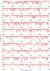 |
Fig. B.1 Mean spectrum of the secondary star in the CD-III range of PEPSI (4800-5400 Å). The black line is the observation, the red line is a model fit based on ParSES and MARCS. |
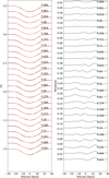 |
Fig. B.2 LSD profiles for the iMAP inversions. On the left panel the observed line profiles (red line) are compared with the fitted synthetic profiles (black dotted lines). The corresponding residuals are plotted in the right panel. Numbers on the right side of each panel indicate the rotational phase. |
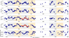 |
Fig. B.3 Chromospheric line emissions and effective temperature versus time. The dark blue circles indicate the STELLA observations while red triangles show the PEPSI dataset. Consecutive complete rotations are shaded with gray and orange colors. |
All Tables
All Figures
|
Fig. 1 Phase-folded radial velocities of both stars in the system. Circles indicate STELLA observations; triangles show PEPSI observations. The green lines (solid and dashed) represent the orbital fit, while the dashed black line marks the center-of-mass velocity. |
| In the text | |
|
Fig. 2 Spectral disentangling by median subtraction. Panel a: the mean spectrum of the secondary star is shown as a black line (top). The composite spectrum (blue) and the primary star spectrum (red) are plotted with a vertical shift of 0.15 at orbital phase 0.82. Panel b: time series composite spectra phase-folded with the orbital period. |
| In the text | |
|
Fig. 3 Radial velocities of HR 7275a from VATT+PEPSI and STELLA+SES. Top panel : SB1 orbital fit is shown as a black line along with the data. Observations from STELLA+SES are indicated with dark blue circles and VATT+PEPSI observations are shown as red triangles. Bottom panel: RV residuals after subtracting predicted orbital velocities. The RV jitter appears multi-peaked per rotation. The thick gray and orange lines highlight two different rotational-modulation models. |
| In the text | |
|
Fig. 4 Lomb-Scargle periodogram (red) of RV residuals from Fig. 3. The strongest peak occurs at half the stellar rotation period, while one-third of the rotation appears prominently as the second strongest peak. Phase dispersion minimization (PDM) is shown in blue, with its strongest peak at 27.2 days. |
| In the text | |
|
Fig. 5 Panel a: Doppler image of HR 7275a. The rotational phases are indicated via phase φ with a sampling of 0.25. Panel b: contemporaneous RV modulation due to spots. Panel c: relative flux modulation of CaIIIRT8542 Å simultaneous to the DI. Dark blue dots represent the STELLA dataset and red triangles indicate the PEPSI observations. |
| In the text | |
|
Fig. 6 Mercator map of the spotted surface of HR 7275a. |
| In the text | |
|
Fig. 7 Disentangled spectrum of HR7275b near Hα (upper panel) and the Ca II IRT region (lower panel). The observed spectrum is shown as a black line, and the model is indicated by a dashed red line. |
| In the text | |
|
Fig. 8 Stokes V magnetic field measurements for HR 7275 from 2024. Panel a: LSD line profiles from PEPSI, in units of normalized intensity. Panel b: integrated Stokes-V profiles, in units of Gauss. |
| In the text | |
|
Fig. 9 Lithium abundance analysis. Panel a: median spectrum of HR 7275a (black dots) and Turbospectrum fit (dashed red line). The gray shaded areas indicate the regions outside the fitting range (white). Panel b: same as panel a, but for HR 7275b. The dashed blue line shows a PEPSI spectrum of 70 Vir. |
| In the text | |
|
Fig. B.1 Mean spectrum of the secondary star in the CD-III range of PEPSI (4800-5400 Å). The black line is the observation, the red line is a model fit based on ParSES and MARCS. |
| In the text | |
|
Fig. B.2 LSD profiles for the iMAP inversions. On the left panel the observed line profiles (red line) are compared with the fitted synthetic profiles (black dotted lines). The corresponding residuals are plotted in the right panel. Numbers on the right side of each panel indicate the rotational phase. |
| In the text | |
|
Fig. B.3 Chromospheric line emissions and effective temperature versus time. The dark blue circles indicate the STELLA observations while red triangles show the PEPSI dataset. Consecutive complete rotations are shaded with gray and orange colors. |
| In the text | |
Current usage metrics show cumulative count of Article Views (full-text article views including HTML views, PDF and ePub downloads, according to the available data) and Abstracts Views on Vision4Press platform.
Data correspond to usage on the plateform after 2015. The current usage metrics is available 48-96 hours after online publication and is updated daily on week days.
Initial download of the metrics may take a while.