| Issue |
A&A
Volume 706, February 2026
|
|
|---|---|---|
| Article Number | A112 | |
| Number of page(s) | 11 | |
| Section | Planets, planetary systems, and small bodies | |
| DOI | https://doi.org/10.1051/0004-6361/202557737 | |
| Published online | 09 February 2026 | |
Astrometric Reconnaissance of Exoplanetary Systems (ARES)
I. Methodology validation with HST point-source images of Proxima Centauri
1
INAF – Osservatorio Astronomico di Padova,
Vicolo dell’Osservatorio 5,
Padova
35122,
Italy
2
Department of Astronomy & Astrophysics, University of California,
San Diego, La Jolla,
California
92093,
USA
★ Corresponding author: This email address is being protected from spambots. You need JavaScript enabled to view it.
Received:
17
October
2025
Accepted:
28
November
2025
Abstract
We present the first results of the Astrometric Reconnaissance of Exoplanetary Systems (ARES) project, aimed at validating and characterizing candidate exoplanets around the nearest systems using multi-epoch Hubble Space Telescope (HST) data. In this first paper, we focus on Proxima Centauri, leveraging archival and recent HST observations in point-source imaging mode. We refined the geometric-distortion calibration of the HST detector used and developed a robust methodology to derive high-precision astrometric parameters by combining HST measurements with the Gaia DR3 catalog. We determined Proxima’s position, proper motion, and parallax with uncertainties at the ~0.4-mas, 50-µas yr−1, and 0.2-mas levels, respectively. This allowed us to achieve consistent results with Gaia measurements within ~1σ. We further investigated the presence of the candidate exoplanet Proxima c by analyzing the proper-motion anomaly derived from combining long-term HST-based and short-term Gaia astrometry. Based on the assumption of a circular, face-on orbit, we obtained an estimated mass of mc = 3.4−3.4+5.2 M⊕, which is broadly consistent with radial-velocity constraints, but still limited by our current uncertainties. These results establish the foundation for the next phase of ARES, which will exploit HST spatial-scanning observations to achieve astrometric precisions of a few tens of µas, while also enabling a direct search for astrometric signatures of low-mass companions.
Key words: astrometry / planets and satellites: detection / stars: low-mass
© The Authors 2026
 Open Access article, published by EDP Sciences, under the terms of the Creative Commons Attribution License (https://creativecommons.org/licenses/by/4.0), which permits unrestricted use, distribution, and reproduction in any medium, provided the original work is properly cited.
This article is published in open access under the Subscribe to Open model. This email address is being protected from spambots. You need JavaScript enabled to view it. to support open access publication.
1 Introduction
Astrometry is a niche technique in the field of exoplanet detection, but it is potentially one of the most informative. The basis of the astrometric method is simple: the mutual gravitational interaction between a host star and its companion(s) makes them orbit around a common center of mass. For the host star, this orbital motion manifests as an astrometric “wobble” that deviates from the star’s normal proper and parallactic motions. Detection of an exoplanet by the host star’s astrometric wobble is similar in nature to the line-of-sight (LOS) radial-velocity (RV) method; however, because astrometric wobble is measured in two spatial dimensions instead of one, it does not suffer from the typical mass-inclination degeneracy of the RV method. In addition, the astrometric method is not affected by other limitations of spectroscopic measurements like spectral-line asymmetries or gravitational redshift. By measuring the deviations from the expected motion of the host star on the sky, we can directly derive the perturber’s mass (if the host mass is known) and its orbital parameters. Alas, the astrometric wobble induced on a host star is proportional to the planet/host star-mass ratio and it is, hence, typically very small; it is also inversely proportional to the distance of the host star to the Earth and, thus, it is only relevant for the closest stars to the Sun.
The Gaia Data Release 3 (DR3) release Gaia Collaboration (2016, 2023) has provided astrometry for more than a billion of sources. The Gaia consortium has run a preliminary search for companions around nearby stars in the unpublished Gaia-DR3 astrometric time series (Holl et al. 2023). However, the least massive objects (brown dwarfs and exoplanets) will be detectable by the astrometric method only around the brightest host stars. Low-mass companions to low-mass stars, the most common type of stars in the Milky Way, are generally too faint for Gaia measurements (Perryman et al. 2014), as is the case for stars in crowded fields or with extreme properties. The release of all the Gaia individual measurements with the DR4 (ca. December 2026) will enable the community to develop new tools to search for planets at the faint end of Gaia ’s sensitivity. However, these detections will be difficult to validate as few other instruments can provide a comparable astrometric precision. Alternative methods and facilities are needed to fill the low-mass gap left by Gaia as well as to independently validate the discoveries Gaia will make. The Astrometric Reconnaissance of Exoplanetary Systems (ARES) project is designed to address this need through a challenging use of Hubble Space Telescope (HST) data. ARES is aimed at validating and characterizing candidate exoplanets orbiting two of the closest systems to the Sun: Proxima Centauri (Proxima) and Luhman 16AB (Luh 16AB).
Proxima is a late-type M dwarf and the closest star to the Sun at ~1.3 pc. It is known to host multiple exoplanets, all found by the LOS RV method. Proxima b (discovered by Anglada-Escudé et al. 2016) has a minimum mass of 1.0 ± 0.1 M⊕, a semi-major axis of ~0.05 AU, and a period of ~11.2 days (Damasso et al. 2020), placing it within Proxima’s habitable zone. Proxima d has a minimum mass of 0.26 ± 0.05 M⊕, a semi-major axis of 0.03 AU, and a period of 5.1 days (Faria et al. 2022). A third exo-planet, Proxima c, was reported by Damasso et al. (2020), with a minimum mass of 5.8 ± 0.1 M⊕, a semi-major axis of ~1.58 AU, and a period of ~1900 days. However, the existence of Proxima c remains uncertain, even after subsequent direct imaging and astrometric observations (Gratton et al. 2020; Kervella et al. 2019, 2020, 2022; Benedict & McArthur 2020). As discussed in Damasso et al. (2020), the existence of Proxima c would be a challenge to various scenarios about the formation of super-Earth exoplanets. Confirming the existence of Proxima c is thus extremely important for exoplanet formation theory.
Luh 16AB is a brown-dwarf binary discovered by Luhman (2013) with the Wide-field Infrared Survey Explorer (WISE). At only ~2 pc from the Sun, Luh 16AB is the closest brown dwarf and brown-dwarf binary to the Sun. Luh 16A is an L8 dwarf with a mass of 35.4 ± 0.2 MJup, while Luh 16B is a T1 dwarf with a mass 29.4 ± 0.2 MJup (both masses from Bedin et al. 2024a). This system straddles the transition between the L dwarf and T dwarf spectral classes, a phase of brown dwarf evolution characterized by significant changes in their atmospheric properties, including the formation of CH4 gas and the depletion of condensate clouds (e.g., Burgasser et al. 2013; Kniazev et al. 2013; Apai et al. 2021). High-precision astro-metric measurements of the system have revealed perturbations of their proper, parallactic, and binary orbital motion, which could be related to a third, unseen body. The combined efforts of Boffin et al. (2014), Lazorenko & Sahlmann (2018) and Bedin et al. (2017, 2024a) have ruled out candidate companions down to Neptunian masses, limited by their astrometric precisions.
The ARES project plans to measure astrometric perturbations in the motion of these systems by unseen companions using multi-epoch HST observations taken with the Ultraviolet and VISible (UVIS) channel of the Wide Field Camera 3 (WFC3). The best techniques in point-source imaging with WFC3/UVIS are able to deliver a precision of ~300–400 µas Bellini & Bedin (2009); Bellini et al. (2011); however, is not sufficient for a statistically significant detection of the astrometric wobble induced by the candidate exoplanets. Instead, we chose to use images obtained using the so-called “spatial scanning” mode, which slews the telescope during the observation and spreads the light along a trail. The many samplings obtained in a trail enable astrometric precisions of tens of µas in a single exposure, far beyond what is possible with HST using the “classical” point-source imaging (e.g., Riess et al. 2014).
This first paper of the series described how we improved the methodology described in Bedin et al. (2017, 2024a) to set up the foundations to fit the astrometric parameters of our targets. Following on this aim, we chose to focus on point-source images of Proxima for which we have a clear understanding of positional precision and systematics. Proxima is bright and well measured in the Gaia DR3 catalog, so we can compare the astrometric parameters derived with our HST data with those from Gaia. Future works will focus on the analysis of the images in spatial-scanning mode, and search for the astrometric signatures of its companions. The paper is organized as follows. In Sect. 2, we introduce the dataset and its reduction using state-of-the-art techniques for precise and accurate astrometry; Sect. 3 provides an overview about the setup of the astrometric reference frame and the differences with past works on the same topic, as well as the fit of the “absolute” astrometric parameters. In Sect. 4, we present an attempt to estimate the mass of Proxima c, combining our and Gaia’s proper motions (PMs). We also discuss the limits of the point-source imaging. Finally, our conclusions and next steps are described in Sect. 5.
Log of observations used in this work.
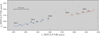 |
Fig. 1 Composite image of Proxima obtained by co-adding all HST exposures, properly normalized, from October 2012 to February 2025. The colored line represents the motion of Proxima predicted by our astrometric fit (see Sect. 3.3), with the color changing from blue to white to red as the epoch increases (see also labels in the plot). North is up and east is to the left. |
2 Data reduction
Proxima Centauri was imaged by HST through several archival and our own proprietary General Observer (GO) programs (Table 1). For this first part of the project, we made use of WFC3/UVIS data taken between 2012 and 2025 in F555W and F467M filters (see Fig. 1). Because of the brightness of Proxima, these images are very short so as not to saturate the target. Unavoidably, the setup of the F555W observations (which were also taken in subarray mode, with only one chip used) limits the number (less than 10 in the worst case) and the signal (up to six magnitudes fainter than Proxima) of the surrounding sources. Given the relatively redder color of Proxima with respect to the other field stars, the choice of the F467M filter in the latest programs leads to a less extreme exposure time for the observations, which results in a less dramatic scene (20–30 reference stars, only three magnitudes fainter than Proxima). In the next section we discuss how these different setups impacted the astrometric registration of our images.
We analyzed calibrated (dark- and bias-subtracted as well as flat-fielded) _flc exposures corrected for charge-transfer-efficiency (CTE) defects, which affects positions and flux of sources in the detector, as described in Anderson & Bedin (2010); Anderson & Ryon (2018). The _flc images are also best suited for astrometry because they are not resampled, thus retaining the real flux distribution of the sources that would be washed out by the mosaicking process in drizzled images (Anderson 2022).
The region of sky currently containing Proxima is sparse, so there is no need for a two-step astro-photometric reduction as in crowded fields (e.g., Libralato et al. 2018, 2022). We run the code hst1pass1 (Anderson 2022) to measure position and flux of all detectable sources in the field by means of a point-spread-function (PSF) fitting. We made use of effective-PSF (ePSF) models obtained by fine-tuning (for each image) publicly-available sets of library ePSFs derived as in Anderson & Bedin (2017). Positions were corrected for geometric-distortion (GD) effects using the WFC3/UVIS GD corrections by Bellini & Bedin (2009); Bellini et al. (2011). The GD of a detector changes over time, even for the instruments on board HST, although at a slower pace. In the next we describe an additional fine-tuning of the GD correction to compensate for these changes, which primarily impacted the more-recent F467M images. Finally, the astro-photometric catalog of each exposure contains a parameter called QFIT, which represents the goodness of the ePSF fit (Libralato et al. 2014; Anderson 2022). Bright, well-measured sources are characterized by a QFIT close to 0, whereas poorly measured and/or faint objects have a larger QFIT value. We used this parameter to discard low-quality Proxima measurements in the astrometric fit stage.
3 Determination of the astrometric parameters
Bedin et al. (2017, 2024b) and Bedin & Fontanive (2018, 2020) have detailed a procedure that makes use of the Gaia catalog to set up a common reference frame to compare multi-epoch observations of a target and fit its astrometric parameters. We followed a similar approach, while implementing some changes and improvements.
3.1 Astrometric reference frame and GD refinement
We used the Gaia DR3 catalog to set up a common reference frame for Proxima’s HST data. We considered only the Gaia sources in our field that fulfilled all the following conditions:

The first condition excludes Proxima itself from the sample. The parallaxes were corrected for the zero-point bias described in Lindegren et al. (2021) using the associated code2. This correction works only for sources with a five- or six-parameter solution, a requirement that is ensured by enforcing the last condition.
For each image, we propagated the Gaia positions in equatorial coordinates to the epoch of the observation. This epoch propagation was performed using the tool PyGaia3, which is designed for Gaia science performance simulation and data manipulation of astrometric catalogs. The repository documentation warns users that this package is not intended for accurate astrometry applications, and that the Astropy (Astropy Collaboration 2013, 2018) facility should be used instead. The PyGaia epoch-propagation routines follow the prescriptions in the official Gaia DR3 documentation (Hobbs et al. 2022), whereas those in Astropy include pieces of software from the International Astronomical Union’s Standard of Fundamental Astronomy (SOFA) repository4. However, the former tool performs much faster than the latter. We compared a set of simulated, epoch-propagated positions of a Proxima-like target (high parallax and PM, with a known LOS velocity) and found that within the temporal baseline covered by our HST observations, the coordinates computed with the two tools differ by 10 µas at most in 20 years, well below the accuracy of our HST data. For this reason, we used PyGaia in our work.
The aforementioned epoch propagation was performed with a linear model (i.e., the standard model of stellar motion), starting from the assumption that stars are moving with uniform velocity relative to the Solar System barycenter. While this model includes effects such as the perspective acceleration, which can be significant for high-PM stars close to the Sun like Proxima, it cannot be directly compared with our observations that are taken from (close to) the Earth at different times of the year, thus including the effect of the annual parallax. We modeled the annual-parallax contribution by adding to the position of the barycenter of the Solar System at a given epoch, based on the following quantity:
![Mathematical equation: $\left[ {\matrix{ {{\rm{\Delta }}\alpha } & {{\rm{\Delta }}\delta } \cr } } \right] = \left[ {\matrix{ {{{\rm{p}}_\alpha }} \cr {{{\rm{p}}_\delta }} \cr } } \right] \cdot \varpi ,$](/articles/aa/full_html/2026/02/aa57737-25/aa57737-25-eq3.png) where ϖ is the parallax and (pα, pδ) denote the parallactic factors computed using the python version of the Naval Observatory Vector Astrometry Software (NOVAS Barron et al. 2011) package5.
where ϖ is the parallax and (pα, pδ) denote the parallactic factors computed using the python version of the Naval Observatory Vector Astrometry Software (NOVAS Barron et al. 2011) package5.
These epoch-propagated equatorial coordinates were then projected on to a tangent plane centered at (α, δ)tan = (217.392321472, −62.676075117); namely, the position of Proxima in the Gaia DR3 catalog (epoch 2016.0). For this purpose, we can use, for instance, Eqs. (3) and (4) in Bedin & Fontanive (2018). These projected coordinates remain in angular units (e.g., degrees), which makes direct comparisons with the pixel-based coordinates in the HST-based catalogs difficult. Therefore, we applied three changes: (i) we divided these projected positions by an arbitrary pixel scale (40 mas pixel−1, which is similar to the pixel scale of the WFC3/UVIS camera); (ii) we flipped the x direction to align the detector’s x axis with the common convention of pointing towards West (the y axis is oriented towards north); and (iii) we added an offset of ∆(x, y) = (5000, 5000) pixels to avoid having to work with negative coordinates. All these choices are completely arbitrary, but necessary to set up a common, pixel-based reference frame that would allow us to transform positions from equatorial coordinates to the pixel-based coordinate system of any given HST image (and vice versa, as described in the next part of the work). We stress that the actual values used for the shift, scale, and orientation do not matter; what is important is that their consistency is maintained throughout the entire process.
We cross-identified the HST-based catalog of each image with the corresponding Gaia-based catalog, prepared as just described above. We collected all HST-Gaia position pairs obtained this way, and used them to refine the GD correction of the WFC3/UVIS detector following the prescriptions of Bellini & Bedin (2009). Any GD correction is derived by comparing a set of observed positions (taken with the detector used to solve for the GD) and a set of distortion-free positions. In our case, the former set corresponds to the HST-based positions, whereas the latter set is provided by the Gaia catalog (see, e.g., Griggio et al. 2023, 2024; Libralato et al. 2024a, for other works that used the Gaia catalog to solve for the GD correction of an imager). The refinement of the WFC3/UVIS GD correction can be summarized as follows.
For each chip, we used four-parameter linear transformations (two offsets, change of global scale, rotation) to transform the Gaia-based positions on to the GD-corrected reference frame of the corresponding HST catalog. The coefficients of such transformations were computed by means of the positions of bright, well-measured stars in both catalogs.
We applied an inverse GD correction to get these transformed Gaia positions in the raw HST reference system.
We defined the positional residuals as the difference between the HST-based and the Gaia-based raw positions.
We modeled these positional residuals (normalized as in Bellini & Bedin 2009) with two third-order polynomial functions, which represent the additional GD correction for the WFC3/UVIS detector.
We added the new GD correction to the original one from Bellini & Bedin (2009) and Bellini et al. (2011).
We iterated the entire process (cross-match and GD correction) ten times, after which we found negligible differences between the polynomial coefficients in two consecutive iterations. The GD refinement for the F555W solution does not provide a significant change, as expected since most of the F555W data was taken a few years after the WFC3/UVIS installation, so that the GD correction from Bellini & Bedin (2009); Bellini et al. (2011) is still optimal. For the F467M filter, we found that the GD changed over time, with small trends as a function of the y position. After the correction, this GD systematic ended up disappearing.
3.2 The catalog of Proxima’s positions
The next step consisted of creating the catalog with the multi-epoch measurements of the position of Proxima. While Proxima’s coordinates in every exposure come directly from the ePSF fit (described in Sect. 2), there are other quantities required prior to move to the next stage: a pixel-to-equatorial coordinate transformation (and its inverse) and an estimate of the positional error of Proxima.
For each, image we cross-identified the same stars and computed the six-parameter linear transformations (similar to the four-parameter transformations with the addition of two so-called skew terms that described the change of scale between x and y axes and the change of perpendicularity between x and y axes) necessary to transform the positions, as measured in the HST reference frame on to that of Gaia (defined as in Sect. 3.1). The coefficients of such transformations were computed by means of the positions of bright, well-measured stars in both catalogs (Proxima excluded). We also ensured that these stars would lie in the same WFC3/UVIS chip as Proxima. As shown in many astrometric works with HST data (e.g., Bellini et al. 2014; Libralato et al. 2018, 2022), a local approach works best in terms of minimizing residual systematics that can affect astrometry. Using stars within the same chip is an appropriate compromise between locality and statistics. Together with the details provided in Sect. 3.1, these transformations contain the necessary information to transform positions between the HST-and Gaia-based pixel reference frame, as well as to the ICRS (in equatorial coordinates), at any given epoch and image.
For the positional-error budget of each estimate of Proxima’s position, we needed to include two contributions: (i) the positional error of Proxima and (ii) the error of the aforementioned transformations. To estimate the former, we used the empirical relation between positional error and magnitude described in Sect. 5.2 and Fig. 2 of Bellini et al. (2014, provided via private communication by the first author). Proxima is very bright (instrumental magnitude ≲−13.5) in all our exposures and the predicted positional error is <0.01 WFC3/UVIS pixel (<0.4 mas). These values are in agreement with the expected positional precision for bright stars in Bellini et al. (2011).
The latter contribution is dominated by the positional error in the HST images of the stars used to compute the coefficients of the linear transformations. We estimated this value by transforming the position of Proxima from the HST-based to the Gaia-based pixel coordinate system using six-parameter linear transformations. The coefficients of these transformations were calculated by adding to each HST position a random noise (drawn from a Gaussian distribution with 0 mean and σ equal to the expected magnitude-dependent error of each star). We repeated this operation 1000 times and defined the error due to the transformations as the standard deviation of all these measurements. The final positional uncertainty for each Proxima measurement was defined as the sum in quadrature of these two errors. This error is, on average, 0.03 WFC3/UVIS pixel. For the F467M data, which have many stars in common between HST and Gaia measured with a relatively-high signal-to-noise ratio, all the measurements have about the same positional uncertainty (0.03 WFC3/UVIS pixel). For the F555W data, which can have fewer than ten stars in common and with a three-to-six magnitudes of difference with Proxima, the uncertainty ranges between 0.02 and 0.06 WFC3/UVIS pixel.
Finally, before determining the astrometric parameters, we analyzed the catalog of Proxima to identify entries with poor quality, looking for each filter at the positional-uncertainty and QFIT values as a function of magnitude. While the F467M data looked consistent, the F555W data showed clear outliers in the distribution. Thus, we excluded all measurements with a positional uncertainty larger than 0.05 WFC3/UVIS pixel (2 mas), and QFIT value larger than 0.07. The latter threshold was defined by visually inspecting the distribution of the QFIT as a function of instrumental magnitude. We noticed a skewed distribution of the QFIT values with average 0.05 and σ ~ 0.02. We chose a conservative cut at 0.07. The QFIT selection was applied only in the direction of increasing QFIT and not the opposite direction (i.e., mean −1σ). This is because a QFIT <0.05 is usually considered the proxy of a well-measured star. In total, the final sample for the astrometric analysis was comprised of 59 2D measurements.
Fitted astrometric parameters for Proxima.
3.3 Determination of the astrometric parameters
The goal of this paper is to determine the astrometric parameters of Proxima at a specific epoch, namely: the equatorial coordinates (αref, δref), the PM (µα cos δ, µδ), and the parallax, ϖ. We chose tref = 2016.0, so that we could directly compare our findings with those in the Gaia DR3 catalog.
We derived these astrometric parameters by comparing our HST measurements with a model representing the expected path of Proxima in the plane of the sky. The model was obtained by combining a linear motion (from PyGaia) and an annual-parallax displacement (using the NOVAS package as described in Sect. 3.1). A more sophisticated model for the stellar motion, such as that provided by PyGaia, is needed to include the effect of the perspective acceleration. In our work, we did not use any LOS RV velocity measurement in the fit, but assumed a constant value of −21.94 km s−1 from the Gaia DR3 catalog.
Proxima differs significantly in both color and magnitude from the adopted network of reference stars used for the alignment; namely, sources in the Gaia DR3 catalog with well-determined PMs and parallaxes. Although using _flc exposures should remove most systematics associated to the magnitude dependence of the CTE (and we will describe later how residual CTE systematic errors are also removed in the process), additional residuals might still arise owing the color difference of the target. In wide-filter passbands, the exact spectral energy distribution (SED) of each star affects both the fine structure of the PSF and the GD of the camera via optical refraction (see, e.g., Bellini et al. 2011, for an example of the relation between GD correction and stars’ SED). These color-dependent effects are equivalent to a form of differential chromatic refraction. We investigated the possible contribution of these effects, finding to be small for Proxima. Nevertheless, we report the results of the astrometric fit with a possible chromatic correction in Appendix A.
We developed our suits for the astrometric fit so that the comparison between observations and models happens in the image plane (specifically, the GD-corrected reference frame of each HST image) instead of the sky plane, in preparation for the analysis of the trailed images in future works. The implementation of this step is trivial because of how we set up our framework in Sect. 3 and it just requires to: (i) project the sky coordinates predicted by the model at any given epoch using the tangent point, (α, δ)tan, provided in Sect. 3.1; and (ii) transform each model position from the projected sky plane to the corresponding image plane of the HST exposure using the six-parameter linear transformations described in Sect. 3.2.
The best-fit astrometric parameters and corresponding errors were obtained by using the affine-invariant Markov Chain Monte Carlo (MCMC) method emcee (Foreman-Mackey et al. 2013). For each parameter, we defined an initial guess using a value close to the Proxima entry in the Gaia DR3 catalog and then allowed it to vary uniformly within a wide range of values (see Table 2). Starting from the initial guesses, we initialized 100 walkers and let them evolve for 5000 steps, maximizing the log-likelihood defined as
![Mathematical equation: $\ln {\cal L} = - {1 \over 2}\left[ {\chi _x^2 + \chi _y^2 + \mathop \sum \limits_{i = 1}^N \ln \left( {2\pi \sigma _x^2} \right) + \mathop \sum \limits_{i = 1}^N \ln \left( {2\pi \sigma _y^2} \right)} \right],$](/articles/aa/full_html/2026/02/aa57737-25/aa57737-25-eq14.png) where N is the number of measurements, (σx, σy) are the positional errors defined in Sect. 3 and
where N is the number of measurements, (σx, σy) are the positional errors defined in Sect. 3 and
 with Oi,
  , and Mi are the observed data-point, the observed uncertainty and the model values (either x or y position), respectively. The best-fit solution was defined the parameter set that maximizes the log-probability, after removing the first 20% of the steps as burn-in phase. The corresponding errors were computed as the 16th and 84th percentiles about the best-fit solution of the posterior distributions.
Working on the x/y image plane allows us to search for systematic trends in the data. The observation-model (O−C) residuals should be, on average, zero regardless the position on the detector where Proxima was imaged. After the first iteration, we noticed that this requirement was not fulfilled, meaning that some unknown systematics and/or the contribution of outliers are affecting our fit. The left-most panels of Fig. 2 shows an overview of the (O−C) x and y residuals at the first iteration of the astrometric fit as a function of (xraw, yraw) position on the detector. The first iteration produced a solution with a scatter that can be as large as 5.8 mas, (~0.14 WFC3/UVIS pixel), which seem to correlate with the position on the detector. These systematics could be related to residual CTE defects (which can be important for the F555W images since their exposure time is 1 s), as well as to chromatic and magnitude effects in the ePSF (Proxima is redder and 3–6 mag brighter than any other source in the field). We corrected these systematics by fitting a linear relation to the (O−C) residuals as a function of xraw/yraw as done by Bedin et al. (2017). This correction was computed separately for each filter.
However, in contrast with Bedin et al. (2017), where the dataset used was homogeneous (multi-epoch data taken with the same instrument, filter, and exposure time) and the observations were designed ad-hoc for their target, for Proxima, we have two distinct datasets. In particular, the 1-s exposures in the F555W filter are the most problematic: there are a dozen stars in the field of Proxima in the best case, so the image alignment (Sect. 3) end up being not as robust as for the F467M filter, resulting in a larger scatter in the (O−C) residuals for the F555W data than for the F467M one. This level of scatter made it difficult to remove bad measurements before the astrometric fit. For this reason, after each iteration we flagged and excluded all measurements that for which the (O−C) x/y residuals from the previous iteration were more than 3σ away from the median value of the residual distribution.
We iterated the entire procedure (astrometric fit, systematic correction, outlier rejection) three times, after which we found no clear systematics in the (O−C) residuals (see rightmost panels of Fig. 2) and the number of outliers did not change in two consecutive iterations (12 out of 59 data points). We estimated the goodness of our fit by computing the reduced chi-square  , where “dof” refers to the degrees of freedom, namely, the difference between the number of data points and the number of fitting parameters. The final
  is 0.41. The best-fit astrometric solution6 is reported in Table 2, and the corner plots are provide in Appendix B. A visual representation of the astro-metric solution of Proxima, together with the (O−C) residuals along (α cos δ, δ) directions, is presented in Fig. 3. Table 2 also reports the values taken from the Gaia DR3 catalog for comparison. The agreement between the two sets of parameters is at the 1σ level in the worst case, with the largest discrepancies being ∆α2016 ~ 0.3 mas and ∆ϖ ~ 0.3 mas. Remarkably, our and Gaia PMs are in agreement within 20 µas yr−1. Our positional and parallax uncertainties are larger than Gaia’s, especially for α2016.0, but in agreement with the typical positional uncertainty of a bright star with HST (0.4 mas ~ 0.01 WFC3/UVIS pixel; Bellini & Bedin 2009; Bellini et al. 2011). Appendix C provides the positions of Proxima used in our analysis.
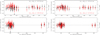 |
Fig. 2 Positional residuals from the model (O−C) as a function of xraw and yraw, respectively from top to bottom. Black points refer to the x residuals, while red points represent the y residuals. The gray dashed line in each plot is set at 0 for reference. The left panels show the O−C at the first iteration of the astrometric fit, while the right panels display the residuals at the last iteration of the fit (less points are visible because of the iterative rejection of outliers; see the text for details). In the top panels, we report the standard deviation (σO−C and the absolute maximum scatter of the points (|∆O−C|) as a reference. |
4 Proper motion anomaly using HIPPARCOS, Gaia, and HST
Our astrometric time series can potentially be used to search for residual astrometric signatures in the (O−C) plane. However, the precision achieved by our point-source images (which can be as large as 1 mas) is comparable to the amplitude of the residuals we want to investigate, making it challenging to draw any conclusion about potential signatures with enough statistical confidence. An alternative method to search for an unseen companion that is commonly used when dedicated astrometric series are not available is the so-called PM anomaly (PMa).
If a star is part of a binary system, its apparent motion in the plane of the sky varies over time due to the gravitational influence of its companion(s). The amplitude of this perturbation depends on the mass of the companion and the overall orbital configuration (e.g., the semi-major axis). The PMa technique is aimed at detecting these deviations by comparing two independent sets of PMs for the source: the long-term PM (in which orbital perturbations average out) and short-term PM (an “instantaneous” measurement of the star’s motion). Kervella et al. (2019) took advantage of the HIPPARCOS and Gaia DR2 catalogs to measure this PMa by comparing the Gaia DR2 (short-term) PM and the HIPPARCOS-Gaia (Hip-Gaia; long-term) PM. Subsequently, Kervella et al. (2022) updated the PMa values with the Gaia DR3 catalog. We followed the prescriptions Kervella et al. (2019, 2022) to compute the PMa by combining our HST long-term PM (temporal baseline of 10.89 yr) with the short-term PM provided by the Gaia DR3 and try to infer the mass of Proxima c, the only putative exoplanet around Proxima for which the PMa method is sensitive.
First, we measured the PMa vector by combining our HST and the Gaia DR3 PMs. This computation has to be done in three dimensions (analogous to the “standard model of linear motion” introduced in Sect. 3.3) to take into account effects such as the parallax and perspective acceleration of Proxima. Our HST-Gaia PMa for Proxima is
 which is similar to what found by Kervella et al. (2022):

Both estimates present a marginal significance. To derive a mass for Proxima c from the PMa, we followed the procedure described in Kervella et al. (2019). This methodology assumes a simplified geometry (a binary system with circular orbit seen with a face-on orientation), meaning that more complex orbital configurations can lead to different solutions. Upon these assumptions, the mass of the companion (m2) scales with the square root of the mass of the primary star (m1) and the observed PMa (∆µ), but it is also degenerate with orbital radius, r:
![Mathematical equation: ${{{m_2}} \over {\sqrt r }} = \sqrt {{{{m_1}} \over G}} \cdot \left( {{{{\rm{\Delta }}\mu \left[ {{\rm{mas y}}{{\rm{r}}^{ - 1}}} \right]} \over {\varpi [{\rm{mas}}]}} \cdot 4740.470} \right),$](/articles/aa/full_html/2026/02/aa57737-25/aa57737-25-eq21.png) where G is the universal gravitational constant, and 4740.470 is a conversion factor from mas yr−1 to m s−1. Kervella et al. (2019) showed that additional factors should be included: the orbital inclination, the time-window smearing of the short-term PM, and the sensitivity of the long-term PM. The first term was defined in a statistical fashion as in Sect. 3.6.1 of Kervella et al. (2019). The smearing factor, necessary to compensate for the fact the short-term PM is not instantaneous but taken over an extended period of time (1038 days for Gaia DR3), was computed as in Sect. 3.6.2 of Kervella et al. (2019). The factor related to the sensitivity of the long-term PM is included so not to bias the PMa vector if the orbital period of the binary system is significantly longer than the long-term-PM temporal baseline. In our work, we assumed the results of the simulations in Sect. 3.6.3 of Kervella et al. (2019) and shown in their Fig. 3, rescaled by our long-term temporal baseline.
where G is the universal gravitational constant, and 4740.470 is a conversion factor from mas yr−1 to m s−1. Kervella et al. (2019) showed that additional factors should be included: the orbital inclination, the time-window smearing of the short-term PM, and the sensitivity of the long-term PM. The first term was defined in a statistical fashion as in Sect. 3.6.1 of Kervella et al. (2019). The smearing factor, necessary to compensate for the fact the short-term PM is not instantaneous but taken over an extended period of time (1038 days for Gaia DR3), was computed as in Sect. 3.6.2 of Kervella et al. (2019). The factor related to the sensitivity of the long-term PM is included so not to bias the PMa vector if the orbital period of the binary system is significantly longer than the long-term-PM temporal baseline. In our work, we assumed the results of the simulations in Sect. 3.6.3 of Kervella et al. (2019) and shown in their Fig. 3, rescaled by our long-term temporal baseline.
Figure 4 shows the expected mass of Proxima c as a function of the orbital radius, assuming a mass of 0.1221 M⊙ for Proxima (Mann et al. 2015). The blue line represents our solution, while the light-blue region sets the 1σ uncertainty on the mass at any given radius, which was computed including the contributions of the PM errors with a Monte Carlo approach. The dashed gold line is the relation derived using the PMa from Kervella et al. (2022, the uncertainty region is omitted for clarity). The spikes at radius lower than 1 AU mark the parameter space in which our PMa is not sensitive. The pink triangle is the minimum mass of Proxima c from the work of Damasso et al. (2020, mc sin i = 5.7 ± 1.9 M⊕); meanwhile, the red point represents the mass measured by Kervella et al. (2020), which used the PMa of Kervella et al. (2019) and the results from Damasso et al. (2020) to estimate the orbital inclination (i = 152 ± 14 deg) and mass of Proxima c  .
.
Assuming a circular orbit for Proxima c with radius equal to the semi-major axis, a = 1.48 AU, from Damasso et al. (2020), we obtained a mass for Proxima c of  . A similar result was obtained considering the PMa from Kervella et al. (2022,
  . We also ran the analysis using the Hip-Gaia long-term PM from Kervella et al. (2022) and a short-term PM obtained using part of the HST data at our disposal (green line in Fig. 4). Specifically, we re-ran our analysis using only the F467M data taken in 2020s. We fixed α2016, δ2016 and ϖ to the values obtained in Sect. 3.3 and just fitted the PM components. These data span a temporal baseline of ~3 yr, similar to that of the Gaia DR3. We found a PM of
 which leads to

Using this value for the PMa, we obtained  . Although all estimates are in agreement at 1σ level with the minimum mass from Damasso et al. (2020), these PMa-based masses of Proxima c are likely biased by a mix of large PM uncertainty and smearing effect of the Gaia DR3 or HST short-term PMs. It is worth noting that recent studies using LOS RVs (e.g., Faria et al. 2022; Suárez Mascareño et al. 2025) have not found clear signatures of Proxima c, further complicating the puzzle. Additional astrometric monitoring is needed to constrain the existence and mass of Proxima c.
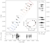 |
Fig. 3 Series of HST observations of Proxima. The main panel shows the path in the (α cos δ, δ) plane of Proxima. The filled black dots are the HST measurements used in the last iteration of the astrometric fit, while the open dots refer to the rejected measurements. The gray, solid line is the expected linear motion (i.e., without the annual-parallax contribution) of Proxima, whereas the colored line represents the astrometric solution of Proxima. The line color changes from blue to white to red as the epoch increases (from the bottom left to the top left of the plot). The inset in the main panel shows the residuals from the linear motion, which highlight the annual-parallax ellipse. The residuals of the astrometric fit as a function of α cos δ/δ coordinates are displayed in the side panels. The gray, dashed line is set to 0 as a reference. In each of these side panels, we report the standard deviation (σO−C and the absolute maximum scatter of the points (|∆O−C|). |
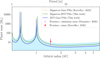 |
Fig. 4 Expected mass of Proxima c as a function of its orbital radius derived from the PMa analysis. The solid blue line shows the mass estimate obtained in this work from the combination of HST and Gaia-DR3 astrometry, with the shaded light-blue region representing the 1σ uncertainty. The relation obtained combining Hip-Gaia (marked just as “HIPPARCOS” in the plot legend for clarity) and part of the HST data is shown as a solid green line. The dashed yellow line represents the PMa-based relation obtained by Kervella et al. (2022) using HIPPARCOS and Gaia. The pink triangle marks the minimum mass derived of Proxima c from Damasso et al. (2020). The red point shows the mass estimate from Kervella et al. (2020). |
5 Conclusions
This first paper of the ARES project presents a refined astrometric analysis of Proxima using multi-epoch HST WFC3/UVIS observations obtained over 13 years. By improving the GD correction of the WFC3/UVIS detector and combining HST and Gaia-DR3 astrometry, we achieved sub-milliarcsecond precision on Proxima’s position, PM, and parallax. Our best-fit solution agrees with that from Gaia DR3 within ~1σ, validating the methodology and error budget. Our measurement also provides an independent test for the Gaia’s astrometry of this very-red M dwarf. Indeed, we linked our astrometry to that of Gaia using all suitable stars in the field except Proxima, and then fit Proxima’s position, PM, and parallax. If our HST or Gaia measurements of Proxima were affected by a color-dependent systematic that made Proxima “behave” differently from the other bluer sources, we expected to find a discrepancy in the astrometric parameters of Proxima determined using HST and Gaia. Since we found no such discrepancy, we conclude that Proxima measurement is robust.
We investigated the presence of the proposed exoplanet Proxima c by measuring the PMa from the combination of HST and Gaia PMs. The PMa method starts from the assumption of a circular and face-on orbit, so the derived mass can be different from the real one depending on the actual planetary architecture. Nevertheless, this method makes it possible to infer the mass of a companion when astrometric time series are not available. We derived a mass estimate of  for an orbital radius of 1.48 AU (i.e., the semi-major axis of Proxima c from past LOS RV analyses), consistent within uncertainties to RV-based measurements, but still limited by the current precision of the PMa method and dataset at our disposal.
This work establishes the foundations for the next phase of ARES. Future studies will exploit HST spatial-scanning observations, capable of reaching astrometric precisions of a few tens of µas per epoch, to directly search for the signatures of low-mass companions around Proxima and other nearby systems. These upcoming results will provide a critical benchmark for validating Gaia-based discoveries and refining our understanding of planetary systems in the solar neighborhood.
The next Gaia data releases will increase and improve the synergy between HST and Gaia. Gaia’s improved astrometric parameters at all magnitudes, including at the faint end, will enlarge the pool of suitable objects available to set up the reference network in studies similar to ours. Smaller uncertainties in positions, PMs and parallaxes will provide more robust epoch-propagated Gaia positions (Sect. 3). However, the HST-Gaia synergy extends beyond mutual support. HST data can complement the Gaia astrometric series by providing additional data points and increasing the temporal baseline for the astrometric fit. Furthermore, the combination of HST and Gaia (regardless of the data release) offers the possibility to yield PMs (and, potentially, parallaxes, depending on the temporal sampling) for sources within an HST field that currently only have a two-parameter solution in the Gaia catalog (e.g., Libralato et al. 2024b; Bedin 2025).
Acknowledgement
M.L. acknowledges support from the “IAF: Astrophysics Fellowships in Italy”. Based on observations with the NASA/ESA HST, obtained at the Space Telescope Science Institute, which is operated by AURA, Inc., under NASA contract NAS 5-26555. This work has made use of data from the European Space Agency (ESA) mission Gaia (https://www.cosmos.esa.int/gaia), processed by the Gaia Data Processing and Analysis Consortium (DPAC, https://www.cosmos.esa.int/web/gaia/dpac/consortium). Funding for the DPAC has been provided by national institutions, in particular the institutions participating in the Gaia Multilateral Agreement. This research made use of astropy, a community-developed core python package for Astronomy (Astropy Collaboration 2013, 2018), emcee (Foreman-Mackey et al. 2013), NOVAS (Barron et al. 2011), pygtc (Bocquet & Carter 2016). This work also employed PyGaia, which is based on the effort by Jos de Bruijne to create and maintain the Gaia Science Performance pages (with support from David Katz, Paola Sartoretti, Francesca De Angeli, Dafydd Evans, Marco Riello, and Josep Manel Carrasco), and benefits from the suggestions and contributions by Morgan Fouesneau, Tom Callingham, John Helly, Javier Olivares, Henry Leung, Johannes Sahlmann.
References
- Anderson, J. 2022, One-Pass HST Photometry with hst1pass, Instrument Science Report ACS 2022-02 [Google Scholar]
- Anderson, J., & Bedin, L. R. 2010, PASP, 122, 1035 [CrossRef] [Google Scholar]
- Anderson, J., & Bedin, L. R. 2017, MNRAS, 470, 948 [NASA ADS] [CrossRef] [Google Scholar]
- Anderson, J., & Ryon, J. E. 2018, Improving the Pixel-Based CTE-correction Model for ACS/WFC, Instrument Science Report ACS 2018-04 [Google Scholar]
- Anglada-Escudé, G., Amado, P. J., Barnes, J., et al. 2016, Nature, 536, 437 [Google Scholar]
- Apai, D., Nardiello, D., & Bedin, L. R. 2021, ApJ, 906, 64 [NASA ADS] [CrossRef] [Google Scholar]
- Astropy Collaboration (Robitaille, T. P., et al.) 2013, A&A, 558, A33 [NASA ADS] [CrossRef] [EDP Sciences] [Google Scholar]
- Astropy Collaboration (Price-Whelan, A. M., et al.) 2018, AJ, 156, 123 [Google Scholar]
- Barron, E. G., Kaplan, G. H., Bangert, J., et al. 2011, AAS Meeting Abstracts, 217, 344.14 [Google Scholar]
- Bedin, L. R. 2025, A&A, 704, A193 [NASA ADS] [CrossRef] [EDP Sciences] [Google Scholar]
- Bedin, L. R., & Fontanive, C. 2018, MNRAS, 481, 5339 [NASA ADS] [CrossRef] [Google Scholar]
- Bedin, L. R., & Fontanive, C. 2020, MNRAS, 494, 2068 [NASA ADS] [CrossRef] [Google Scholar]
- Bedin, L. R., Pourbaix, D., Apai, D., et al. 2017, MNRAS, 470, 1140 [NASA ADS] [CrossRef] [Google Scholar]
- Bedin, L. R., Dietrich, J., Burgasser, A. J., et al. 2024a, Astron. Nachr., 345, e20230158 [NASA ADS] [Google Scholar]
- Bedin, L. R., Dietrich, J., Burgasser, A. J., et al. 2024b, Astron. Nachr., 345, e20230158 [NASA ADS] [Google Scholar]
- Bellini, A., & Bedin, L. R. 2009, PASP, 121, 1419 [CrossRef] [Google Scholar]
- Bellini, A., Anderson, J., & Bedin, L. R. 2011, PASP, 123, 622 [CrossRef] [Google Scholar]
- Bellini, A., Anderson, J., van der Marel, R. P., et al. 2014, ApJ, 797, 115 [Google Scholar]
- Benedict, G. F., & McArthur, B. E. 2020, Res. Notes Am. Astron. Soc., 4, 86 [Google Scholar]
- Bocquet, S., & Carter, F. W. 2016, J. Open Source Softw., 1, 46 [NASA ADS] [CrossRef] [Google Scholar]
- Boffin, H. M. J., Pourbaix, D., Mužić, K., et al. 2014, A&A, 561, L4 [NASA ADS] [CrossRef] [EDP Sciences] [Google Scholar]
- Burgasser, A. J., Sheppard, S. S., & Luhman, K. L. 2013, ApJ, 772, 129 [Google Scholar]
- Damasso, M., Del Sordo, F., Anglada-Escudé, G., et al. 2020, Sci. Adv., 6, eaax7467 [Google Scholar]
- Faria, J. P., Suárez Mascareño, A., Figueira, P., et al. 2022, A&A, 658, A115 [NASA ADS] [CrossRef] [EDP Sciences] [Google Scholar]
- Foreman-Mackey, D., Hogg, D. W., Lang, D., & Goodman, J. 2013, PASP, 125, 306 [Google Scholar]
- Gaia Collaboration (Prusti, T., et al.) 2016, A&A, 595, A1 [NASA ADS] [CrossRef] [EDP Sciences] [Google Scholar]
- Gaia Collaboration (Vallenari, A., et al.) 2023, A&A, 674, A1 [NASA ADS] [CrossRef] [EDP Sciences] [Google Scholar]
- Gratton, R., Zurlo, A., Le Coroller, H., et al. 2020, A&A, 638, A120 [EDP Sciences] [Google Scholar]
- Griggio, M., Nardiello, D., & Bedin, L. R. 2023, Astron. Nachr., 344, easna.20230006 [NASA ADS] [Google Scholar]
- Griggio, M., Libralato, M., Bellini, A., et al. 2024, A&A, 687, A94 [NASA ADS] [CrossRef] [EDP Sciences] [Google Scholar]
- Hobbs, D., Lindegren, L., Bastian, U., et al. 2022, Gaia DR3 documentation Chapter 4: Astrometric data, Gaia DR3 documentation, European Space Agency; Gaia Data Processing and Analysis Consortium [Google Scholar]
- Holl, B., Sozzetti, A., Sahlmann, J., et al. 2023, A&A, 674, A10 [NASA ADS] [CrossRef] [EDP Sciences] [Google Scholar]
- Kervella, P., Arenou, F., Mignard, F., & Thévenin, F. 2019, A&A, 623, A72 [NASA ADS] [CrossRef] [EDP Sciences] [Google Scholar]
- Kervella, P., Arenou, F., & Schneider, J. 2020, A&A, 635, L14 [NASA ADS] [CrossRef] [EDP Sciences] [Google Scholar]
- Kervella, P., Arenou, F., & Thévenin, F. 2022, A&A, 657, A7 [NASA ADS] [CrossRef] [EDP Sciences] [Google Scholar]
- Kniazev, A. Y., Vaisanen, P., Mužić, K., et al. 2013, ApJ, 770, 124 [Google Scholar]
- Lazorenko, P. F., & Sahlmann, J. 2018, A&A, 618, A111 [NASA ADS] [CrossRef] [EDP Sciences] [Google Scholar]
- Libralato, M., Bellini, A., Bedin, L. R., et al. 2014, A&A, 563, A80 [NASA ADS] [CrossRef] [EDP Sciences] [Google Scholar]
- Libralato, M., Bellini, A., van der Marel, R. P., et al. 2018, ApJ, 861, 99 [CrossRef] [Google Scholar]
- Libralato, M., Bellini, A., Vesperini, E., et al. 2022, ApJ, 934, 150 [NASA ADS] [CrossRef] [Google Scholar]
- Libralato, M., Argyriou, I., Dicken, D., et al. 2024a, PASP, 136, 034502 [Google Scholar]
- Libralato, M., Bedin, L. R., Griggio, M., et al. 2024b, A&A, 692, A96 [NASA ADS] [CrossRef] [EDP Sciences] [Google Scholar]
- Lindegren, L., Bastian, U., Biermann, M., et al. 2021, A&A, 649, A4 [EDP Sciences] [Google Scholar]
- Luhman, K. L. 2013, ApJ, 767, L1 [NASA ADS] [CrossRef] [Google Scholar]
- Mann, A. W., Feiden, G. A., Gaidos, E., Boyajian, T., & von Braun, K. 2015, ApJ, 804, 64 [Google Scholar]
- Perryman, M., Hartman, J., Bakos, G. Á., & Lindegren, L. 2014, ApJ, 797, 14 [Google Scholar]
- Riess, A. G., Casertano, S., Anderson, J., MacKenty, J., & Filippenko, A. V. 2014, ApJ, 785, 161 [Google Scholar]
- Sahu, K. C., Bond, H. E., Anderson, J., & Dominik, M. 2014, ApJ, 782, 89 [NASA ADS] [CrossRef] [Google Scholar]
- Suárez Mascareño, A., Artigau, É., Mignon, L., et al. 2025, A&A, 700, A11 [NASA ADS] [CrossRef] [EDP Sciences] [Google Scholar]
- Zurlo, A., Gratton, R., Mesa, D., et al. 2018, MNRAS, 480, 236 [NASA ADS] [CrossRef] [Google Scholar]
Proxima passed close to faint background sources around epochs 2014.8 and 2016.2, causing microlensing events that shifted these star positions (Sahu et al. 2014; Zurlo et al. 2018). These sources are not included in the network of objects used to setup our reference frame (Sect. 3.1) because they are not visible in the F555W data (>8.5 mag fainter than Proxima), so we anticipate no impact on our analysis. To confirm this, we re-measured Proxima’s astrometric parameters excluding the images taken near these events. The parameters were consistent with those from the full sample at the 0.5σ level, except for the parallax, which showed consistency at ~2σ. The parallax changed the most because the excluded 2014.8 images are near the maximum parallax elongation, making them crucial for constraining that parameter.
Appendix A Astrometric fit with chromatic-correction terms
Fitted astrometric parameters for Proxima with the chromatic-correction terms.
 |
Fig. B.1 1D (histograms) and 2D (marginalized) projections of the posterior-probability distributions of the astrometric parameters of Proxima. The dashed, gray lines set the best-fit parameters (also reported, with the corresponding uncertainties, above each histogram). The marginalized projections of the posterior-probability distributions show 1, 2, and 3 σ contour in different shades of blue. |
As discussed in Sect. 3.3, we tested the inclusion of an empirical correction. We did not attempt to disentangle the chromatic effects individually, but rather to model their combined impact on the measured centroid of the target relative to the reference star network (with a different mean color), as a function of the detector orientation of each HST exposure with respect to the absolute reference frame set by Gaia. To this end, we introduced two additional free parameters in the astrometric fit, describing the orientation and amplitude of the corresponding systematic vector in the detector plane:
![Mathematical equation: $\left[ {\matrix{ {{\rm{\Delta }}{\alpha _{{\rm{color}}}}} & {{\rm{\Delta }}{\delta _{{\rm{color}}}}} \cr } } \right] = \left[ {\matrix{ {{k_\alpha }} & {{k_\delta }} \cr } } \right] \cdot \left[ {\matrix{ {{{\sin \theta } \over {\cos (\delta )}}} \cr {\cos \theta } \cr } } \right],$](/articles/aa/full_html/2026/02/aa57737-25/aa57737-25-eq36.png) where (kα, kδ) are the amplitudes of the correction along the (α, δ) directions, and θ is the position angle of the image (computed using the six-parameter linear transformations described in Sect. 3.2). The 1/ cos δ term is needed to compensate for the projection effects. Accounting for this systematic contribution leads to a slightly improved fit for Proxima, although with larger errors for some of the astrometric parameters.
where (kα, kδ) are the amplitudes of the correction along the (α, δ) directions, and θ is the position angle of the image (computed using the six-parameter linear transformations described in Sect. 3.2). The 1/ cos δ term is needed to compensate for the projection effects. Accounting for this systematic contribution leads to a slightly improved fit for Proxima, although with larger errors for some of the astrometric parameters.
We report in Table A.1 the results of the astrometric fit with the chromatic-correction terms in the model. The final  is 0.48. The agreement with Gaia is slightly better (0.5-σ level). The largest discrepancies are again ∆α2016 ~ 0.1 mas and ∆ϖ ~ 0.2 mas. Convergence of the astrometric-fit process was reached in six iterations, and the number of rejected measurements in the process was 9. Using this solution and the same prescriptions detailed in Sect. 4, for Proxima c, we obtained a mass of
  .
.
Appendix B Corner plots
Figure B.1 displays the corner plots of the final fit of the astrometric parameters of Proxima described in Sect. 3.3.
Appendix C Observed positions of Proxima
Table C.1 provides the measurements of Proxima included in our fit, together with other useful quantities. We provide both the pixel-based positions corrected for GD in each image (i.e., those actually used in Sect. 3.3) and the corresponding equatorial coordinates.
Proxima’s measurements used in our work.
All Tables
All Figures
|
Fig. 1 Composite image of Proxima obtained by co-adding all HST exposures, properly normalized, from October 2012 to February 2025. The colored line represents the motion of Proxima predicted by our astrometric fit (see Sect. 3.3), with the color changing from blue to white to red as the epoch increases (see also labels in the plot). North is up and east is to the left. |
| In the text | |
|
Fig. 2 Positional residuals from the model (O−C) as a function of xraw and yraw, respectively from top to bottom. Black points refer to the x residuals, while red points represent the y residuals. The gray dashed line in each plot is set at 0 for reference. The left panels show the O−C at the first iteration of the astrometric fit, while the right panels display the residuals at the last iteration of the fit (less points are visible because of the iterative rejection of outliers; see the text for details). In the top panels, we report the standard deviation (σO−C and the absolute maximum scatter of the points (|∆O−C|) as a reference. |
| In the text | |
|
Fig. 3 Series of HST observations of Proxima. The main panel shows the path in the (α cos δ, δ) plane of Proxima. The filled black dots are the HST measurements used in the last iteration of the astrometric fit, while the open dots refer to the rejected measurements. The gray, solid line is the expected linear motion (i.e., without the annual-parallax contribution) of Proxima, whereas the colored line represents the astrometric solution of Proxima. The line color changes from blue to white to red as the epoch increases (from the bottom left to the top left of the plot). The inset in the main panel shows the residuals from the linear motion, which highlight the annual-parallax ellipse. The residuals of the astrometric fit as a function of α cos δ/δ coordinates are displayed in the side panels. The gray, dashed line is set to 0 as a reference. In each of these side panels, we report the standard deviation (σO−C and the absolute maximum scatter of the points (|∆O−C|). |
| In the text | |
|
Fig. 4 Expected mass of Proxima c as a function of its orbital radius derived from the PMa analysis. The solid blue line shows the mass estimate obtained in this work from the combination of HST and Gaia-DR3 astrometry, with the shaded light-blue region representing the 1σ uncertainty. The relation obtained combining Hip-Gaia (marked just as “HIPPARCOS” in the plot legend for clarity) and part of the HST data is shown as a solid green line. The dashed yellow line represents the PMa-based relation obtained by Kervella et al. (2022) using HIPPARCOS and Gaia. The pink triangle marks the minimum mass derived of Proxima c from Damasso et al. (2020). The red point shows the mass estimate from Kervella et al. (2020). |
| In the text | |
|
Fig. B.1 1D (histograms) and 2D (marginalized) projections of the posterior-probability distributions of the astrometric parameters of Proxima. The dashed, gray lines set the best-fit parameters (also reported, with the corresponding uncertainties, above each histogram). The marginalized projections of the posterior-probability distributions show 1, 2, and 3 σ contour in different shades of blue. |
| In the text | |
Current usage metrics show cumulative count of Article Views (full-text article views including HTML views, PDF and ePub downloads, according to the available data) and Abstracts Views on Vision4Press platform.
Data correspond to usage on the plateform after 2015. The current usage metrics is available 48-96 hours after online publication and is updated daily on week days.
Initial download of the metrics may take a while.