| Issue |
A&A
Volume 706, February 2026
|
|
|---|---|---|
| Article Number | A313 | |
| Number of page(s) | 11 | |
| Section | Galactic structure, stellar clusters and populations | |
| DOI | https://doi.org/10.1051/0004-6361/202557973 | |
| Published online | 23 February 2026 | |
The stellar to sub-stellar masses transition in 47 Tuc
1
INAF, Observatory of Rome,
Via Frascati 33,
00077
Monte Porzio Catone (RM),
Italy
2
Osservatorio Astronomico di Padova,
Vicolo dell’Osservatorio 5,
35122
Padova,
Italy
3
Dipartimento di Fisica e Astronomia Augusto Righi, Università degli Studi di Bologna,
Bologna,
Italy
4
Dipartimento di Fisica e Astronomia “Galileo Galilei”, Univ. di Padova,
Padova,
Italy
5
Dipartimento di Matematica e Fisica, Università degli Studi Roma Tre,
via della Vasca Navale 84,
00100
Roma,
Italy
★ Corresponding author: This email address is being protected from spambots. You need JavaScript enabled to view it.
Received:
4
November
2025
Accepted:
14
December
2025
Abstract
Context. The study of the globular cluster 47 Tuc offers an opportunity to shed new light on the debated issue of the presence of multiple populations in globular clusters, as recent results from HST photometry and high-resolution spectroscopy outlined star-to-star differences in the surface chemical composition.
Aims. The goal of the present investigation is the interpretation of recent JWST data of the low main sequence of 47 Tuc, in order to explore the stellar to sub-stellar transition, derive the mass distribution of the individual sources, and disentangle stars from different populations.
Methods. Stellar evolution modelling of low-mass stars of metallicity [Fe/H] = −0.78 and oxygen content [O/Fe] = +0.4 and [O/Fe] = 0 was used to simulate the evolution of the first and the second generation of the cluster. The comparison between the calculated sequences with the data points was used to characterise the individual objects, split the different stellar components, and infer the current mass function of the cluster.
Results. The first generation of 47 Tuc harbours ~45% of the overall population of the cluster, the remaining 55% making up the second generation. The transition from the stellar to the sub-stellar domain is found at 0.074 M ⊙ and 0.07 M⊙ for the first and second generations, respectively. The mass function of both stellar generations is consistent with a Kroupa-like profile down to ~0.22 M⊙.
Key words: stars: abundances / stars: evolution / stars: interiors / globular clusters: individual: NGC 104
© The Authors 2026
 Open Access article, published by EDP Sciences, under the terms of the Creative Commons Attribution License (https://creativecommons.org/licenses/by/4.0), which permits unrestricted use, distribution, and reproduction in any medium, provided the original work is properly cited.
This article is published in open access under the Subscribe to Open model. This email address is being protected from spambots. You need JavaScript enabled to view it. to support open access publication.
1 Introduction
Observational evidence collected in the last decades demonstrates beyond any reasonable doubt that the majority of Galactic globular clusters (GC), if not all of them, harbour two or more stellar populations, differing in the distribution of the light element abundance (Kraft 1994; Gratton et al. 2019; Milone & Marino 2022) and, as has been deduced by the interpretation of the morphology of the horizontal branch (HB) and from the detection of multiple main sequences (MSs), of the helium mass fraction (Norris 1981; D'Antona et al. 2002; Lee et al. 2005; D'Antona et al. 2005; Piotto et al. 2007; D'Antona & Caloi 2008; Tailo et al. 2020; D'Antona et al. 2022).
These findings stimulated a lively debate regarding the action of a self-enrichment mechanism operating soon after the formation of GC, such that new stellar generations (second generation, hereinafter 2G) formed from the ashes of stars belonging to the first, original population (1G). Several candidates have been proposed as possible pollutants of the intra-cluster medium that might trigger the formation of multiple populations; namely, fast-rotating massive stars (Decressin et al. 2007), massive binaries (de Mink et al. 2009), super-massive stars (Denissenkov & Hartwick 2014), and massive AGBs (Ventura et al. 2001). The difficulties encountered by the various scenarios in accounting for the results of the observations were extensively discussed by Renzini et al. (2015).
The investigations of this argument have traditionally focused on the interpretation of two main aspects: on the one hand the MS spread, the one observed in the red giant branch (RGB); on the other hand the morphology of the HB. These two aspects, in combination with the chemical patterns derived from high-resolution spectroscopy, are fundamental to infer information on the presence of multiple populations in a given GC, and to trace the history of the star formation during the infancy of the cluster. The most recent years have witnessed the development of a new method, based on appropriate combinations of magnitudes in different filters, which proves extremely powerful in disentangling different stellar populations evolving in a given GC (Milone et al. 2015, 2017; Milone & Marino 2022).
The advent of HST allowed us to extend the observations of GC stars to the low MS, down to the brown dwarf domain (Bedin et al. 2001; Richer et al. 2002, 2006, 2008). The interpretation of low-mass (Μ < 0.2 M⊙) star data provides additional information regarding the presence of multiple populations in GC. Indeed, the spectral energy distribution (SED) of these objects is extremely sensitive to variations in element abundances, due to the relevant role that molecular chemistry plays in the thermal stratification of low-temperature atmospheres (Marley et al. 2002). Furthermore, low-mass stars are fully convective and are exposed to minimal nuclear processing, given the long timescales of hydrogen burning. The study of a brown dwarf is equally interesting: unlike its higher-mass counterparts (Μ > 0.07 M⊙) that reach the conditions for stable hydrogen burning, these objects undergo a gradual cooling process, evolving to lower effective temperatures and luminosities. The decrease in effective temperature favours the formation of complex chemical compounds in the atmospheres, which eventually condense into liquid and solid states, with the formation of clouds (Lunine et al. 1986). The extreme sensitivity of the spectra to chemical composition and age makes the analysis of the brown dwarf a potentially efficient tool to discriminate among different stellar populations and to infer the age of GC.
Interesting studies focused on the chemical diversity of GC stars in the M < 0.2 M⊙ mass domain have been published; for example, by Dotter et al. (2015); Gerasimov et al. (2022a,b). Recent studies on the lower MS of M4 (Milone et al. 2014) and NGC 6752 (Milone et al. 2019) revealed that the relative distribution of stars belonging to different stellar generations deduced from the analysis of the upper MS and the RGB also characterises the lower MS. Dondoglio et al. (2022) showed that the fraction of stars in the different populations of NGC 2808 is constant throughout the mass range extending up to ~0.2 M⊙.
The innovative advent of JWST has further extended the possibility of investigating the very low mass domain of GCs, rendering possible a detailed photometry of the stellar populations down to the brown dwarf domain. In this regard, Marino et al. (2024a, hereinafter MA24) have recently presented JWST data for 47 Tuc, covering the mass domain below ~0.1 M⊙. A thorough interpretation of the dataset by MA24 was hampered by the lack of M < 0.1 M⊙ stellar models, calculated for the chemical composition of the different stellar populations of 47 Tuc.
To overcome this difficulty, we calculated stellar models of mass M ≥ 0.06 M⊙ of the same metallicity of 47 Tuc, based on two different oxygen contents, chosen to span the ~0.4 dex spread in [O/Fe] indicated in MA24. We used these results to characterise the sources observed in terms of mass and chemical composition. Part of the effort is dedicated to reconstructing the present-day mass function (MF) of the 1G and 2G of the cluster across the discontinuity between the stellar and sub-stellar domains.
The paper is organised as follows. A description of the ATON code for stellar evolution used to calculate the evolutionary sequences, and the physical and chemical ingredients adopted, is presented in Section 2. The results obtained, with a discussion of the role of non-greyness and of the separation of the sequences of stars with different chemistry in the most relevant colour-magnitude planes considered, are presented in Sect. 3. In Sect. 4, we derive the MF for the low MS and the transition masses, and in Sect. 5 we summarise and speculate on the results.
2 Numerical, physical, and chemical inputs
The stellar models used in the present work were calculated by means of the ATON code for stellar evolution, in the version described in Ventura et al. (1998). Although the structures of the lowest-mass stars and brown dwarfs are very simple, as they are fully convective, and therefore are close to polytropic structures, in principle, their study is actually hampered by a large number of uncertainties, explored over the years by more and more sophisticated approaches (see, e.g. Kumar 1963; Hayashi & Nakano 1963; D’Antona & Mazzitelli 1985; Nelson et al. 1986; Burrows et al. 1993; Baraffe et al. 1995; Montalbán et al. 2000, to quote only the historical paths.). The uncertainties come from two different difficulties.
First, below ~4000K the atmospheric structure is increasingly dominated by complex molecules. Thus, the atmospheric structure - and its temperature-density stratification - requires the complex physics of band formation to be included. The calculation of atmospheric non-grey opacities is also complicated by the possible complex role of condensates (e.g. Burgasser et al. 2002b). The evolution with decreasing Teff of the molecular band strength defines the classic M, L, T spectral types in the population I brown dwarfs (Kirkpatrick et al. 1999; Burgasser et al. 2002a,b), but it is still not fully understood in recent observations of the MS end of population II GCs (starting from Dieball et al. 2016, for the lowest MS in the cluster M4) and the associated model computation especially developed by Gerasimov et al. (2020). The results for NGC 6397 (Scalco et al. 2024b) and NGC 6752 (Scalco et al. 2024a) are now complemented by those of 47 Tuc (Scalco et al. 2025). Difficult issues such as the role of condensates (Burgasser et al. 2002b; Gerasimov et al. 2024) must be calibrated on the observations themselves. For the lowest masses, non-ideal effects are also important in the atmospheric region.
The second problem concerns the role of the equation of state (EOS) adopted to describe the interior. The most used EOS is at present the one developed by (Saumon et al. 1995, SCVh EOS) for pure hydrogen, pure helium, and pure carbon, for which the necessary intermediate compositions are obtained by the additive volume law, including considering carbon as an ‘average’ metal. Only more recently was a new EOS for pure H and pure He calculated by Chabrier et al. (2019), and it is still subject to the problem that it does not account for the interactions between the two species (see, e.g. the discussion in Montalbán et al. 2000).
We tackled the first problem by adopting as boundary conditions the atmosphere sets computed by Gerasimov et al. (2024). The reason for this choice is twofold. First, the atmospheric grids by Gerasimov et al. (2024) were calculated for the values [α∕Fe] = 0, +0.4, which bracket the range of α-enhancements deduced from the observations of 47 Tuc stars (Marino et al. 2016): this allows for a thorough analysis in width of the cluster MS across the various colour-magnitude diagrams considered. Furthermore, the use of boundary conditions by Gerasimov et al. (2024) allows for a straightforward comparison between the results obtained in the present work and those by Scalco et al. (2025), which are also based on the atmospheric models by Gerasimov et al. (2024).
For the EOS, we used the tables of the ATON code (Ventura et al. 1998) for which the real gas regime was also computed for H-He mixtures, by matching the EOS by Iglesias & Rogers (1996, (OPAL)) - including its updates until 2007 - with tables at high density computed following Stolzmann & Bloecker (1996); Stolzmann & Blöcker (2000). A full description of the EOS tables is given in Ventura et al. (2008).
The evolutionary sequences were started from an early evolutionary pre-MS phase, corresponding to the central temperature of 5 × 10⁵ K, and were extended until the end of core hydrogen burning; for objects not reaching full support by nuclear energy generation, the computations were stopped for ages <50 Gyr, or below the threshold covered by the atmospheric grids (at Teff = 500 K). The range of masses is in the 0.06-0.8 M⊙ domain1.
We computed two sets of models, taking advantage of the available atmospheric grids by Gerasimov et al. (2024). The first set assumes the standard chemical composition of the 1G of 47 Tuc, namely [Fe/H] = −0.78, and alpha enhancement of [a/Fe] = +0.4 (Marino et al. 2016). Based on the solar mixture by Asplund et al. (2009), these values correspond to the metallicity Z = 0.0047. The initial helium is taken as Y = 0.255. A second set of tracks simulates the evolution of the stars belonging to the 2G of 47 Tuc: in this case we assume a depletion in the oxygen content, so that [O/Fe] = 0 (Marino et al. 2016), and a helium mass fraction of Y = 0.30, in agreement with the analysis of the spread of helium in 47 Tuc by Milone et al. (2018).
We considered different locations of the matching region between the interior and the exterior, located at optical depth τ = 1,3,10,100, as was described in detail in Montalbán et al. (2004). We finally adopted τ=10 as boundary for the interior computations, as a compromise to have a good description of the non-grey atmosphere and the necessity of having an EOS including the correct description of the real gas for the smallest masses.
The reason why we limit our exploration to [O/Fe] = 0 and [O/Fe] = +0.4 is because these are the oxygen abundances for which the model atmospheres by Gerasimov et al. (2024) are available. This limitation prevents a more detailed study of the different stellar populations in 47 Tuc, but it proves sufficient to undertake a broad distinction between 1G and 2G stars and to investigate the behaviour of models at the bottom of the MS. For the sake of comparison, we also computed the evolutions for a grey atmosphere, whereby the matching of the results from the solution of the equations of stellar equilibrium from the interior and those from the modelling of the atmosphere was done at the optical depth τ = 2/3.
3 Results
The low MS structures, according to the arguments discussed in the previous section, demand the use of detailed non-grey atmospheric and sub-atmospheric modelling. Furthermore, when the HR diagram is moved to the observational planes, the effects of the absorption bands related to the presence of many specific molecular species, particularly water, affect the relation between the effective temperature of the star and the SED. In this section we first discuss the differences between the results obtained with the grey and non-grey treatments of the external regions, then we focus on the possibility of disentangling the multiple populations of 47 Tuc by interpreting the distribution of the stars in the colour-magnitude diagram.
3.1 The role of non-greyness in the theoretical HR diagram
Fig. 1 shows the position on the HR diagram at the age of 12 Gyr of grey (squares) and non-grey (triangles) stellar models for masses in the 0.08-0.6 M⊙ range. For the lowest masses below 0.08 M⊙, we show the evolutionary tracks covering the ages from 8 to 12 Gyr, with the location at 12 Gyr indicated. For clarity reasons, for the non-grey models we show the τ = 10 case only, as the results obtained with different τ are extremely similar (within 20 K) each other.
The MS luminosity decreases with the stellar mass for Μ ≥ 0.08 M⊙: H-burning sets at ~6.4 × 10⁻² L⊙ for Μ = 0.5 M⊙; ~7.6 × 10⁻³L⊙ for M = 0.2M⊙;-1.3 × 10⁻³ L⊙ for M = 0.1M⊙. The lower mass domain is characterised by the growing influence of core electron degeneracy, which prevents efficient heating of the central regions following the increase in densities. In the very low-mass domain the central temperatures are low enough that H-burning is fully inhibited, and the brown dwarfs cool along approximately constant radius sequences with decreasing luminosities. There is a very small range of masses in which pp burning is ignited, but the nuclear luminosity is not able to fully support the stellar luminosity, and these ‘transition objects’ slowly decrease in luminosity on timescales of a billion years (D’Antona & Mazzitelli 1985) (see Fig. 2).
The main effect of non-greyness in the theoretical HR diagram of Fig. 1 is that M > 0.1 M⊙ stellar models are cooler than the grey counterparts. This is particularly important for 0.10.2 M⊙ stars, for which the differences, ∆Teff, in the effective temperature are slightly below −500 K. For higher masses, we find that ∆Teff is - 250 K at 0.5 M⊙ (and nearly the same for 0.6 M⊙), then becomes negligible for higher masses. The differences are due to the fact that the Eddington approximation results in an atmospheric profile substantially cooler and denser than the non-grey profile, so a hotter effective temperature matches the internal adiabatic stratification, as has been extensively discussed in the literature (see e.g. Chabrier & Baraffe 1997).
The treatment of the boundary conditions also affects the threshold mass separating the stars that reach the MS from those that follow a sub-stellar behaviour, evolving along a constant radius track towards fainter luminosities. The threshold mass is −0.08 M⊙ and −0.073 M⊙ for the grey and non-grey cases, respectively2. The impact of non-greyness tends to vanish in the sub-stellar domain, as the evolution of these stars, which runs along constant radius sequence, is essentially determined by the stellar mass. Non-grey model atmospheres are the fundamental input to derive colours anyway, and in the following we deal only with the non-grey models, whose inputs are described in Section 2.
In Fig. 1 the most interesting and well-known feature is the gap in luminosity at the boundary between stars and transition masses, which catches the eye as a sudden increase in the luminosity difference between adjacent models for the same mass difference (compare the luminosity gap between the 0.08 M⊙ and 0.07 M⊙ non-grey models and the much smaller gap between the 0.08 M⊙ and 0.09 M⊙ model).
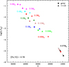 |
Fig. 1 Full points represent the position on the HR diagram of grey (squares) and non-grey (triangles) stellar models with mass in the 0.070.6 M⊙ range, at the age of 12 Gyr. The colour highlights the same mass of the two sequences. For grey stellar models of mass 0.07 M⊙ and 0.08 M⊙, and for the non-grey 0.07 M⊙ model, the evolution in the age range from 8 to 12 Gyr is displayed, the points indicating the position at 12 Gyr. |
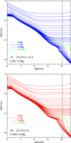 |
Fig. 2 Time variation of the luminosity of stellar models calculated with the physical and chemical input described in Section 2. Stellar models representing the 1G and the 2G of the cluster are shown in the top and bottom panel, respectively. The dashed green line indicates the age of 12 Gyr. The tracks in green highlight the time evolution of the minimum mass supported by proton-proton chain luminosity at the age of 12 Gyr; namely, 0.074 M⊙ (top panel, 1G) and 0.070 M⊙ (bottom panel, 2G). The tracks of the stars of mass 0.2 M⊙ (dotted lines), 0.1 M⊙ (dash-dotted), and 0.08 M⊙ (dashed) are highlighted. |
3.2 Structure and evolution of 1G and 2G stars
The temporal evolution in the luminosity of 1G and 2G stellar models is shown in Fig. 2. The luminosity decreases during the initial evolutionary stages, when the stars are supported by gravitational contraction3. The global behaviour is sensitive to the mass of the star, particularly whether the mass is above the threshold required to start H burning. The tracks reported in Fig. 2 show a clear separation between the higher masses, in which stable hydrogen burning is activated and the luminosity remains constant, and the smaller masses, in which the hydrogen burning power (Lnuc) remains lower the stellar luminosity so that it continues to decrease. The minimum mass reaching Lnuc = Ltot is 0.074 M⊙ for 1G and 0.070 M⊙ for 2G. This difference in mass can be attributed to the different initial helium mass fractions for the two sets of models. To verify this, we compared models with the same helium content, Y=0.255, of 1G and 2G, and found that the atmospheric boundary conditions were not very different despite the very different [O/Fe] content of the two mixtures. We also computed 2G models for different Y values and report the colours and luminosities of the minimum mass that reach the Lnuc = Ltot condition in Table 1. The minimum masses and luminosities decrease slightly with increasing helium content.
The luminosity differences between stellar models of the same mass belonging to the two generations decrease from −40%, for 0.3-0.5 M⊙ stars, to −20%, down to 0.1 M⊙. The differences increase again in the low-mass domain, because the threshold masses for the ignition of hydrogen differ, and thus stars of the same mass behave differently when the transition between the stellar and the sub-stellar domain is approached.
The time evolution of the luminosity for the lowest mass range examined shows also a non-linear behaviour dependent on the treatment of the equation of state into these high-density-low-temperature structures. The interior structure of the stellar models of different mass taken at the age of 12 Gyr is shown in Fig. 3 for both 1G and 2G.
The regions of molecular hydrogen and helium partial ionisation are highlighted in the figures, together with the region in which the real gas effects become important in the structure. The latter region is limited by the lines of temperature and pressure ionisation. The drops in the central temperature below M = 0.073 M⊙ (top panel of Fig. 3, 1G) and M = 0.07 M⊙ (bottom panel, 2G) characterise the transition between the stellar and sub-stellar regime, and it appears clear in the figures that, in addition to the boundary conditions, the EOS description in the real gas regime may also affect the mass location of the transition.
Figures Fig. 2 and mostly Fig. 3 show in an interesting way the transition between stars and brown dwarf regimes. The masses plotted below M = 0.08 M⊙ are spaced by 0.001 M⊙, and we see that in the log(T) versus log(ρ) plane they are first very close together, then more distant, and finally very close again. The region in which they become more distant corresponds to the transition between stellar and sub-stellar structures, which is covered by a very small range of masses, −5 × 10⁻³ M⊙.
3.3 Disentangling the stellar populations in the low main sequence
The difference in the oxygen content between the stars belonging to the 1G and 2G of 47 Tuc, though not particularly relevant for the determination of the position of the stars in the theoretical HR diagram, definitively affects the distribution in the observational colour-magnitude diagrams, specifically in those using filters overlapping with the absorption features associated with the presence of oxygen-bearing molecules (primarily water). Such features are deeper in the spectra of 1G stars, given the higher oxygen mass fraction, than in the 2G counterparts. This effect arises at effective temperatures below 4000 K, becoming more and more important as Teff decreases (Gerasimov et al. 2024).
Following Milone et al. (2023) and MA24, we focused on the (mF115W - mF322W2, mF322W2) and (mF150W - mF322W2, mF322W2) colour-magnitude diagrams. This combination of filters maximises the impact of the oxygen variation between the populations, as the filters cover the spectral region where the flux difference between 1G and 2G stars is at its maximum.
The flux of 2G stars is higher than that of 1G stars in the spectral region covered by the H2O bands, the differences being of the order of 30%. The largest differences are found in the wavelength intervals λ ~ 2.6-2.8 μm, including the median wavelength of the F322w2 filter.
Tables A.1 and A.2 report the effective temperature and luminosity of the model stars belonging to 1G and 2G of the cluster, respectively, the (mF115W - mF322W2) and (mF150W - mF322W2) colours, and mF322W2, at the age of 12 Gyr. The last two columns in the tables give the fraction luminosity of the star due to protonproton reactions at the age of 12 Gyr (unity means that the star reaches stable core H-burning conditions), and the maximum value attained by the same quantity during the evolution.
In Fig. 4, we show the distribution of 47 Tuc sources by MA24 in the (mF115W - mF322W2, mF322W2) diagram. Cluster members along the low MS, reported as yellow points, have been selected according to the indication coming from the proper motions, as is reported in Milone et al. (2023) and MA24. In a nutshell, we selected as cluster members all stars brighter than the mF115W = 26.1 mark, for which the proper motion has a low uncertainty, and on the left of the DR = 2.1 mark. We also included in the CMD stars that do not have proper motions yet: these sources are indicated with cyan dots in Fig. 44.
Overlapping with the data points we report the 12 Gyr isochrones for the 1G and the 2G population of the cluster: solid squares along each isochrone indicate the position of stellar models of a given mass. A satisfactory agreement between the theoretical isochrones and the data points was obtained by assuming reddening E(B - V) = 0.03 and distance modulus (m - M)0 = 13.3: this choice allowed us to reproduce the excursion towards the red of the data points at mF322W2 > 24.
Starting from the brighter region of the plane, the 1G and 2G sequences first move approximately vertically, down to mF322w2 ~ 24: 1G stars are ~0.2 mag bluer than the 2G counterparts, due to the deeper water absorption feature centred at 2.7 μm, which damps the mF322w2 flux, making (mFn5w -mF322w2) redder. We note a slight trend towards the blue in the 23 < mF322w2 < 24 region, as the effective temperature of the stars populating that part of the plane approaches ~2200 K, where the SED peaks in the spectral region at 1.1-1.2 μm.
Both the 1G and the 2G MSs turn to the red for mF322w2 magnitudes above ~24, attained by stars of a mass below 0.08 M⊙, characterised by effective temperatures below 2000 K: this is due to the formation of condensate species (clouds), which favours the shift of the SED to longer wavelengths. The 1G and 2G sequences return to the blue for mF322w2 > 25.5, as a consequence of the gravitational settling of the clouds, which are gradually removed from the atmosphere.
For a better understanding of the colour excursion of the isochrones across the (mFn5w - mF322w2, mF322w2) plane, we show in the top panel of Fig. 6 several spectra at different temperatures (from 2000 K to 500 K and at fixed gravity), while in the middle panel we show the logarithm of their ratio (note that we have taken the 1000 K as reference). We clearly see that the depression caused by water molecules gets deeper as the spectra gets colder. To show why this is relevant for our data, in the bottom panel we plot the throughputs of selected JWST filters5 that fall into the wavelength range of the observed photometric catalogues. Indeed, as we see from the figure, the F322W2 filter intercepts most of the depression, providing a satisfactory explanation to the behaviour we see in our models. This behaviour is the continuation of that already studied in hotter stars (>3000 K) with observed spectra in this cluster (Marino et al. 2024b) and in others (see e.g. Milone et al. 2019, in NGC 6752 with HST).
On general grounds the behaviour of the stellar colours MF115W-MF322W2 is well reproduced, although not perfectly, by the sets of model atmospheres we are using, implying that the way Gerasimov et al. (2024) include condensate species (clouds) in the model is adequate. Indeed use of these atmospheres allows to reproduce: a) the shift to the red of these colours at Teff < 2000 K, not predicted by gas-only models; b) the shift to the blue at Teff < 1500 K, due to the gravitational settling of the clouds, gradually removing them from the atmosphere. Nevertheless, it would be too much to infer the goodness of the qualitative difference between the two sets of models adopted for 1G and 2G. In particular, the observed MS in this plane shows a broadening consistent with the difference between the two sets of isochrones, but precisely at Teff ~ 2000 K the 1G models that have 0.09 ≤ M/M⊙ ≤ 0.075 do not seem to have a plausible correspondence in the data, as they traverse only a few points of the sample. It looks like the different populations merge into a single sequence corresponding to the 2G model location. This merging appears to occur indeed also in the models, but only after reaching the reddest colours, and the broad data in the magnitude range MF322W = 25-276 seem to correspond to the models shifting to the blue due to the cloud settling.
The left side of Fig. 5 shows the distribution of the stars of the cluster in the (mF150W - mF322W2, mF322W2) plane. The blue and red lines indicate the 12 Gyr isochrones for the 1G and 2G stars, respectively, while the full points correspond to the same masses indicated in Fig. 4. We note the significant deviation of the isochrones from the observed sequence in the region of the plane around mF322W2 ~ 24, where the isochrones are far from reproducing the discontinuity in the observed MS. This discrepancy between the theoretical modelling and the data points was recently noticed by Scalco et al. (2025), who demonstrated that a satisfactory fit of the data point in this plane can be obtained only by assuming that the surface chemical composition of the stars at the age of the cluster changes with the stellar mass. This conclusion stems from the fact that reproducing the observations of the very low MS requires the presence of CH4 molecules, which suggests a smaller surface abundance of oxygen in the stars of lower mass; this is the sine qua non condition for the formation of CH4 molecules at the expense of CO. Scalco et al. (2025) propose that the smaller abundance oxygen might be connected to the depletion of oxygen atoms onto dust grains. We leave this problem open.
Transition mass and properties for different chemistries.
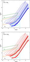 |
Fig. 3 Thermodynamic structure of the stellar models of different mass at the age of 12 Gyr, in the density - temperature plane. The boundaries of the partial helium and partial hydrogen ionisation regions are shown, as well as the region in which corrections to the ideal gas EOS become important, limited at high density by the pressure ionisation boundary. The top panel refers to 1G models; the bottom panel to 2G. The same structures highlighted in Fig. 2 are highlighted here. Below 0.08 M⊙ the mass step is 0.001 M⊙. This allows one to see how fast in mass steps the transition between stars and brown dwarfs is. |
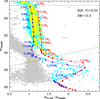 |
Fig. 4 mF322W2 versus (mFn5W - mF322W2) colour-magnitude diagram of 47 Tuc stars from Milone et al. (2023) and MA24. Cyan dots indicate all sources observed for 47 Tuc, yellow dots indicate confirmed cluster members according to the criteria described in Section 3.3, and grey dots indicate SMC members. The blue and the red lines indicate 12 Gyr isochrones for the 1G and 2G of the cluster, respectively. Some specific masses are labelled along the isochrones. The masses 0.5,0.4,0.3,0.25,0.2,0.15,0.12,0.1,0.09,0.085,0.08 M⊙ are shown. Below 0.08 M⊙ the models are spaced by 0.001 M⊙ down to 0.06 M⊙ for the 1G and to 0.058 M⊙ for the 2G. Finally, the upper dashed green line represents the saturation limit (mF322W2 ≃ 18.5), while the lower diagonal green line indicates the limit where proper motions are available (mpn5w = 26.1 as in MA24, properly converted in mF322W2). |
4 The mass function of 47 Tuc
To build the MF for 47 Tuc, Φ(M) (where Φ(M) × dM gives the number of stars with mass in the (M, M + dM) range), we convolved the luminosity function (dN/dmF322W2, LF) in the F322W2 filter by MA24, based on the number counts of the stars within mF322W2 bins 0.4 mag wide, with the mass-mF322W2 relations obtained for the 1G and the 2G of the cluster at the age of 12 Gyr, shown in Fig. 7. Therefore, we have
 (1)
(1)
The LF considered takes into account the corrections for completeness, given in MA24.
If we assume that all the stars reported in Fig. 4 belong to the 1G or the 2G, we obtain the MF shown in the top panel of Fig. 8. For both stellar populations, we note an increasing trend towards the low-mass domain, down to ~0.2-0.3 M⊙, then an approximately constant MF for M < 0.2 M⊙. The minimum of the MF at ~0.8 M⊙, and the rise in the very low-mass domain, are determined by the oscillating behaviour of the LF, which exhibits a deep minimum at mF322W2 ~ 25, then a steep rise at higher F322W2 magnitudes.
As a further step, we attempted to construct separate MFs for the 1G and the 2G. Following MA24, we started with the assumption that 1G stars account for 42% of the overall population of 47 Tuc, while the residual 58% is composed of 2G stars. This is averaged between the two fields examined by MA24. As a second step, we considered the possibility that these percentages can slightly change according to the regions of the plane considered, as a possible consequence of the different slopes of the mass-mF322W2 relations for 1G and 2G stars, which are shown in Fig. 7: indeed the runs of mF322W2 with the mass of the two groups of stars are extremely similar for masses above 0.25 M⊙, while in the lower mass domain the 2G relation is steeper, and thus in a given mF322W2 bin the mass range spanned by 2G stars is narrower than the 1G. Therefore, we allowed the fraction of 1G stars to increase from 42% at mF322W2 = 22.5 to 44% at mF322W2 = 23.5 (we note here that this is still within the errors of the values given by MA24). In this way, we obtained the MFs shown in the right panel of Fig. 8. Both 1G and 2G MFs are consistent with a Kroupa-like profile slope 1.1. Regarding the M < 0.08 M⊙ mass range, both in the 1G and 2G cases, we note a significant increase in the MF, which reflects the notable increase in the number of sources populating the faintest mF322W2 bins, as is clear in Fig. 4.
The last points of the MFs shown in Fig. 8 rely on the hypothesis that the increase in the number of stars shown by the empirical LF is indeed real, as was found by MA24. Obviously it is very awkward to believe in a sharp increase of the MF in a very small range of brown dwarf masses, unless they correspond to the transition region from stars to brown dwarfs, as is suggested by MA24, where the mass luminosity relation has a sharp change of slope. Let us assume, then, that the MF is flat for M < 0.2 M⊙, as is shown in the bottom panel of Fig. 8, and look at the derivative of the mass-F322W2 magnitude relation of the models. The result, for both 1G and 2G models, is shown on the right side of Fig. 5, normalised to the upper part of the luminosity function. We see that the behaviour of the stellar models implies a sharp decrease in the number of stars during the transition from the stellar to the brown dwarf regime, but at smaller masses the brown dwarf simple cooling causes a new increase in the LF, similar to the increase in the empirical LF, but occurring ~ 1.5 mag dimmer. In view of the uncertainties in the models, we suggest that it is possible that the transition from the stellar to the BD regime is indeed what we are witnessing in the data. If the small mass interval of the transition masses is indeed located at mF322W ~ 24, it could also better justify the apparent lack of 1G stars noticed when discussing Fig. 4.
The present findings are based on empirical arguments related to the continuity of the MF of 1G and 2G populations of 47 Tuc. For a more reliable calculation of the MF in the very low-mass domain, both a theoretical effort in the study of model atmospheres and a further observational effort for membership determination by proper motions of the faintest stars populating the bottom of the MS are needed.
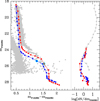 |
Fig. 5 Colour-magnitude data in the (mF150W2 — mF322W2, mF322W2) plane (left, grey dots) are compared with the theoretical models. Contrary to the previous diagram, the agreement is unsatisfactory. These are the data from which the luminosity function was derived. The LF is shown in the right side of the figure (grey dots), together with the theoretical luminosity function obtained by assuming a flat MF below 0.3 M⊙, by normalising the mass luminosity derivative of the models to the data. The figure shows that the observational LF would be reproduced if the transition masses were more luminous than computed by about 1.5 mag. |
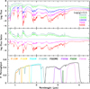 |
Fig. 6 Top panel : synthetic spectra of various temperatures at the labelled gravity; their chemistry and elements distribution correspond to the 1G case. Middle panel : ratio between the spectra showed in the top panel and the one at 1000 K, taken as reference. Bottom panel : throughput of several JWSR filters that are important for the wavelength range of our data. |
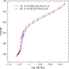 |
Fig. 7 mF322W2 versus logarithm of the mass relation defined by 1G (blue line) and 2G (red) stellar models. |
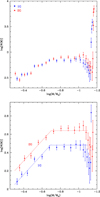 |
Fig. 8 Mass function of the two stellar populations of 47 Tuc. The top panel shows the MF derived under the hypothesis that all the stars either belong to the 1G (blue dots) or belong to the 2G (red dots) of the cluster. The bottom panel reports the MF based on the assumption that 40% of 47 Tuc stars belong to the 1G. This percentage increases to 46% for F322W2 > 21. Both MFs are consistent with a Kroupa-like profile with slope 1.1 down to masses ~0.22 M⊙, then stay constant until the very low-mass domain. |
5 Conclusions
We used recent JWST data of 47 Tuc to study the bottom of the MS of the cluster, with particular care to the still poorly explored transition from the stellar to the sub-stellar domain. With this aim, we calculated evolutionary sequences of M ≥ 0.06 M⊙ stars with metallicity [Fe/H] = −0.78, based on the non-grey treatment of the atmospheric and sub-atmospheric layers. The different stellar populations of 47 Tuc were investigated by adopting oxygen with [O/Fe] = +0.4, to represent the 1G, and stellar models with [O/Fe] = 0, to simulate the 2G of the cluster.
We discuss in detail the transition between stars - masses fully sustained by p-p burning - and brown dwarfs - masses that do not ignite hydrogen due to electron degeneracy. The intermediate transition masses are supported by p-p burning for billions of years, but finally cool as brown dwarfs, as was shown in seminal computations by D’Antona & Mazzitelli (1985). We show that the mass range covered by transition masses is very small, and this produces a dip in the derivative of the mass luminosity relation.
We find a slight mass difference between the threshold value separating the stellar and the sub-stellar domains, the last ones permanently burning central hydrogen are 0.074 M⊙ for the 1G and 0.071 M⊙ for the 2G. A satisfactory agreement between the isochrones and the data points in the (mF115W - mF322W2, mF322W2) colour-magnitude diagram is obtained with reddening E(B - V) = 0.03 and distance modulus (m - M)0 = 13.21. Theoretical isochrones successfully reproduce the colour spread of the MS in the mF322W2 < 23 region of the plane, as well as the upturn to the red in the fainter region of the diagram. In particular, these results indicate that the 1.3 < (mF115W - mF322W2) < 2.2 region at mF322W2 > 24 is populated by M ≤ 0.08 M⊙ stars, which represent the gradual transition from the stellar to substellar domain. We speculate on the possibility that this transition from the star to brown dwarf domain actually occurs at a higher luminosity: this would provide a better agreement between the observed colour-magnitude diagrams and the isochrones and a better agreement with the rising of the LF at the dimmest magnitudes, and with the apparent disappearance of the 1G sequence when the MS rapidly turns to redder colours.
Acknowledgements
This work is based on observations made with the NASA/ ESA/CSA James Webb Space Telescope. The data were obtained from the Mikulski Archive for Space Telescopes (MAST) at the Space Telescope Science Institute, which is operated by the Association of Universities for Research in Astronomy, Inc., under NASA contract NAS 5-03127 for JWST. These specific observations analysed are associated with program JWST-GO-2560 and they can be accessed via doi: 10.17909/6t82-4360. CV acknowledges support by the INAF-fellowship 2024 “Asteroseismological properties of red giant and clump stars” and support by the INAF-fellowship 2025 “Web services and imaging data reduction for LBT”. PV acknowledges support by the INAF-Theory-GRANT 2022 “Understanding mass loss and dust production from evolved stars”. This work has been funded by the European Union - NextGenerationEU RRF M4C2 1.1 (PRIN 2022 2022MMEB9W: “Understanding the formation of globular clusters with their multiple stellar generations”, CUP C53D23001200006). (PI Anna F. Marino).
References
- Asplund, M., Grevesse, N., Sauval, A. J., & Scott, P. 2009, ARA&A, 47, 481 [CrossRef] [Google Scholar]
- Baraffe, I., Chabrier, G., Allard, F., & Hauschildt, P. H. 1995, ApJ, 446, L35 [NASA ADS] [CrossRef] [Google Scholar]
- Bedin, L. R., Anderson, J., King, I. R., & Piotto, G. 2001, ApJ, 560, L75 [NASA ADS] [CrossRef] [Google Scholar]
- Burgasser, A. J., Kirkpatrick, J. D., Brown, M. E., et al. 2002a, ApJ, 564, 421 [NASA ADS] [CrossRef] [Google Scholar]
- Burgasser, A. J., Marley, M. S., Ackerman, A. S., et al. 2002b, ApJ, 571, L151 [NASA ADS] [CrossRef] [Google Scholar]
- Burrows, A., Hubbard, W. B., Saumon, D., & Lunine, J. I. 1993, ApJ, 406, 158 [NASA ADS] [CrossRef] [Google Scholar]
- Chabrier, G., & Baraffe, I. 1997, A&A, 327, 1039 [NASA ADS] [Google Scholar]
- Chabrier, G., Mazevet, S., & Soubiran, F. 2019, ApJ, 872, 51 [NASA ADS] [CrossRef] [Google Scholar]
- D’Antona, F., & Caloi, V. 2008, MNRAS, 390, 693 [CrossRef] [Google Scholar]
- D’Antona, F., & Mazzitelli, I. 1985, ApJ, 296, 502 [CrossRef] [Google Scholar]
- D’Antona, F., Caloi, V., Montalbán, J., Ventura, P., & Gratton, R. 2002, A&A, 395, 69 [CrossRef] [EDP Sciences] [Google Scholar]
- D’Antona, F., Bellazzini, M., Caloi, V., et al. 2005, ApJ, 631, 868 [Google Scholar]
- D’Antona, F., Milone, A. P., Johnson, C. I., et al. 2022, ApJ, 925, 192 [CrossRef] [Google Scholar]
- de Mink, S. E., Pols, O. R., Langer, N., & Izzard, R. G. 2009, A&A, 507, L1 [NASA ADS] [CrossRef] [EDP Sciences] [Google Scholar]
- Decressin, T., Meynet, G., Charbonnel, C., Prantzos, N., & Ekström, S. 2007, A&A, 464, 1029 [NASA ADS] [CrossRef] [EDP Sciences] [Google Scholar]
- Denissenkov, P. A., & Hartwick, F. D. A. 2014, MNRAS, 437, L21 [Google Scholar]
- Dieball, A., Bedin, L. R., Knigge, C., et al. 2016, ApJ, 817, 48 [NASA ADS] [CrossRef] [Google Scholar]
- Dondoglio, E., Milone, A. P., Renzini, A., et al. 2022, ApJ, 927, 207 [NASA ADS] [CrossRef] [Google Scholar]
- Dotter, A., Ferguson, J. W., Conroy, C., et al. 2015, MNRAS, 446, 1641 [Google Scholar]
- Gerasimov, R., Homeier, D., Burgasser, A., & Bedin, L. R. 2020, RNAAS, 4, 214 [Google Scholar]
- Gerasimov, R., Burgasser, A., Homeier, D., et al. 2022a, in American Astronomical Society Meeting Abstracts, 240, 331.04 [Google Scholar]
- Gerasimov, R., Burgasser, A. J., Homeier, D., et al. 2022b, ApJ, 930, 24 [NASA ADS] [CrossRef] [Google Scholar]
- Gerasimov, R., Burgasser, A. J., Caiazzo, I., et al. 2024, ApJ, 961, 139 [NASA ADS] [CrossRef] [Google Scholar]
- Gratton, R., Bragaglia, A., Carretta, E., et al. 2019, A&A Rev., 27, 8 [Google Scholar]
- Hayashi, C., & Nakano, T. 1963, Prog. Theor. Phys., 30, 460 [CrossRef] [Google Scholar]
- Iglesias, C. A., & Rogers, F. J. 1996, ApJ, 464, 943 [NASA ADS] [CrossRef] [Google Scholar]
- Kirkpatrick, J. D., Reid, I. N., Liebert, J., et al. 1999, ApJ, 519, 802 [NASA ADS] [CrossRef] [Google Scholar]
- Kraft, R. P. 1994, PASP, 106, 553 [Google Scholar]
- Kumar, S. S. 1963, ApJ, 137, 1121 [Google Scholar]
- Lee, Y.-W., Joo, S.-J., Han, S.-I., et al. 2005, ApJ, 621, L57 [NASA ADS] [CrossRef] [Google Scholar]
- Lunine, J. I., Hubbard, W. B., & Marley, M. S. 1986, ApJ, 310, 238 [NASA ADS] [CrossRef] [Google Scholar]
- Marino, A. F., Milone, A. P., Casagrande, L., et al. 2016, MNRAS, 459, 610 [NASA ADS] [CrossRef] [Google Scholar]
- Marino, A. F., Milone, A. P., Legnardi, M. V., et al. 2024a, ApJ, 965, 189 [NASA ADS] [CrossRef] [Google Scholar]
- Marino, A. F., Milone, A. P., Renzini, A., et al. 2024b, ApJ, 969, L8 [Google Scholar]
- Marley, M. S., Seager, S., Saumon, D., et al. 2002, ApJ, 568, 335 [NASA ADS] [CrossRef] [Google Scholar]
- Milone, A. P., & Marino, A. F. 2022, Universe, 8, 359 [NASA ADS] [CrossRef] [Google Scholar]
- Milone, A. P., Marino, A. F., Bedin, L. R., et al. 2014, MNRAS, 439, 1588 [NASA ADS] [CrossRef] [Google Scholar]
- Milone, A. P., Marino, A. F., Piotto, G., et al. 2015, ApJ, 808, 51 [NASA ADS] [CrossRef] [Google Scholar]
- Milone, A. P., Piotto, G., Renzini, A., et al. 2017, MNRAS, 464, 3636 [Google Scholar]
- Milone, A. P., Marino, A. F., Renzini, A., et al. 2018, MNRAS, 481, 5098 [NASA ADS] [CrossRef] [Google Scholar]
- Milone, A. P., Marino, A. F., Bedin, L. R., et al. 2019, MNRAS, 484, 4046 [NASA ADS] [CrossRef] [Google Scholar]
- Milone, A. P., Marino, A. F., Dotter, A., et al. 2023, MNRAS, 522, 2429 [CrossRef] [Google Scholar]
- Montalbán, J., D’Antona, F., & Mazzitelli, I. 2000, A&A, 360, 935 [Google Scholar]
- Montalbán, J., D’Antona, F., Kupka, F., & Heiter, U. 2004, A&A, 416, 1081 [NASA ADS] [CrossRef] [EDP Sciences] [Google Scholar]
- Nelson, L. A., Rappaport, S. A., & Joss, P. C. 1986, ApJ, 311, 226 [Google Scholar]
- Norris, J. 1981, ApJ, 248, 177 [Google Scholar]
- Piotto, G., Bedin, L. R., Anderson, J., et al. 2007, ApJ, 661, L53 [NASA ADS] [CrossRef] [Google Scholar]
- Renzini, A., D’Antona, F., Cassisi, S., et al. 2015, MNRAS, 454, 4197 [Google Scholar]
- Richer, H. B., Brewer, J., Fahlman, G. G., et al. 2002, ApJ, 574, L151 [Google Scholar]
- Richer, H. B., Anderson, J., Brewer, J., et al. 2006, Science, 313, 936 [NASA ADS] [CrossRef] [PubMed] [Google Scholar]
- Richer, H. B., Dotter, A., Hurley, J., et al. 2008, AJ, 135, 2141 [NASA ADS] [CrossRef] [Google Scholar]
- Saumon, D., Chabrier, G., & van Horn, H. M. 1995, ApJS, 99, 713 [NASA ADS] [CrossRef] [Google Scholar]
- Scalco, M., Gerasimov, R., Bedin, L. R., et al. 2024a, Astron. Nachr., 345, e20240018 [NASA ADS] [Google Scholar]
- Scalco, M., Libralato, M., Gerasimov, R., et al. 2024b, A&A, 689, A59 [NASA ADS] [CrossRef] [EDP Sciences] [Google Scholar]
- Scalco, M., Gerasimov, R., Bedin, L. R., et al. 2025, A&A, 694, A68 [NASA ADS] [CrossRef] [EDP Sciences] [Google Scholar]
- Stolzmann, W., & Bloecker, T. 1996, A&A, 314, 1024 [Google Scholar]
- Stolzmann, W., & Blöcker, T. 2000, A&A, 361, 1152 [Google Scholar]
- Tailo, M., Milone, A. P., Lagioia, E. P., et al. 2020, MNRAS, 498, 5745 [CrossRef] [Google Scholar]
- Ventura, P., Zeppieri, A., Mazzitelli, I., & D’Antona, F. 1998, A&A, 334, 953 [Google Scholar]
- Ventura, P., D’Antona, F., Mazzitelli, I., & Gratton, R. 2001, ApJ, 550, L65 [CrossRef] [Google Scholar]
- Ventura, P., D’Antona, F., & Mazzitelli, I. 2008, Ap&SS, 316, 93 [CrossRef] [Google Scholar]
The choice of starting point has no effect on the conclusions reached, considering that in the low-mass domain explored in the present work the duration of early evolutionary phases is negligible when compared to that of the MS lifetime. Also, for stars in the sub-stellar mass domain the starting point of the evolution is not relevant, because the cooling timescales are of the order of a few gigayears, while the initial contraction phase during which the central temperature increased proceeds with timescales below 108 yr.
Thus, in Fig. 1, we show the evolution of the 0.08 M⊙ grey stellar model, while for the non-grey counterpart of the same mass, we show only the MS location at 12 Gyr.
Below 0.2 M⊙, the initial deuterium burning phase lasts for 2Myr or longer, and appears in the figure as a temporary pause in luminosity during the contraction phase.
We note that Scalco et al. (2025) limit their analysis to M ≥ 0.1 M⊙, corresponding to mF322W2 ≤ 23 mag. This choice is related to the set of isochrones adopted, which unlike ours do not extend down to beyond the transition from the stellar to the non-stellar domain, and to the availability of direct spectroscopic estimates of the chemical abundances of very low-mass stars.
Although the proper motions of these stars are not available, they were considered as cluster members and included in the analysis, following Milone et al. (2023) and MA24, who concluded that the stars in that part of the CMD as probable BDs, with some not relevant contamination from the MC, and foreground or background objects. Their inclusion is further justified by the identification by MA24 of two candidate BDs in that specific range of colours and magnitude values (see their Figure 4). Solving this possible ambiguity would require further observational explorations by the JWST of that region of the CMD in order to obtain accurate proper motion estimates.
Appendix
Table A.1 and Table A.2 below show the values for 47 Tuc 1G and 2G isochrones, based on stellar evolutionary models of different masses (specifications in the notes).
Theoretical and observational quantities for 47 Tuc 1G isochrone
Theoretical and observational quantities for 47 Tuc 2G isochrone
All Tables
All Figures
|
Fig. 1 Full points represent the position on the HR diagram of grey (squares) and non-grey (triangles) stellar models with mass in the 0.070.6 M⊙ range, at the age of 12 Gyr. The colour highlights the same mass of the two sequences. For grey stellar models of mass 0.07 M⊙ and 0.08 M⊙, and for the non-grey 0.07 M⊙ model, the evolution in the age range from 8 to 12 Gyr is displayed, the points indicating the position at 12 Gyr. |
| In the text | |
|
Fig. 2 Time variation of the luminosity of stellar models calculated with the physical and chemical input described in Section 2. Stellar models representing the 1G and the 2G of the cluster are shown in the top and bottom panel, respectively. The dashed green line indicates the age of 12 Gyr. The tracks in green highlight the time evolution of the minimum mass supported by proton-proton chain luminosity at the age of 12 Gyr; namely, 0.074 M⊙ (top panel, 1G) and 0.070 M⊙ (bottom panel, 2G). The tracks of the stars of mass 0.2 M⊙ (dotted lines), 0.1 M⊙ (dash-dotted), and 0.08 M⊙ (dashed) are highlighted. |
| In the text | |
|
Fig. 3 Thermodynamic structure of the stellar models of different mass at the age of 12 Gyr, in the density - temperature plane. The boundaries of the partial helium and partial hydrogen ionisation regions are shown, as well as the region in which corrections to the ideal gas EOS become important, limited at high density by the pressure ionisation boundary. The top panel refers to 1G models; the bottom panel to 2G. The same structures highlighted in Fig. 2 are highlighted here. Below 0.08 M⊙ the mass step is 0.001 M⊙. This allows one to see how fast in mass steps the transition between stars and brown dwarfs is. |
| In the text | |
|
Fig. 4 mF322W2 versus (mFn5W - mF322W2) colour-magnitude diagram of 47 Tuc stars from Milone et al. (2023) and MA24. Cyan dots indicate all sources observed for 47 Tuc, yellow dots indicate confirmed cluster members according to the criteria described in Section 3.3, and grey dots indicate SMC members. The blue and the red lines indicate 12 Gyr isochrones for the 1G and 2G of the cluster, respectively. Some specific masses are labelled along the isochrones. The masses 0.5,0.4,0.3,0.25,0.2,0.15,0.12,0.1,0.09,0.085,0.08 M⊙ are shown. Below 0.08 M⊙ the models are spaced by 0.001 M⊙ down to 0.06 M⊙ for the 1G and to 0.058 M⊙ for the 2G. Finally, the upper dashed green line represents the saturation limit (mF322W2 ≃ 18.5), while the lower diagonal green line indicates the limit where proper motions are available (mpn5w = 26.1 as in MA24, properly converted in mF322W2). |
| In the text | |
|
Fig. 5 Colour-magnitude data in the (mF150W2 — mF322W2, mF322W2) plane (left, grey dots) are compared with the theoretical models. Contrary to the previous diagram, the agreement is unsatisfactory. These are the data from which the luminosity function was derived. The LF is shown in the right side of the figure (grey dots), together with the theoretical luminosity function obtained by assuming a flat MF below 0.3 M⊙, by normalising the mass luminosity derivative of the models to the data. The figure shows that the observational LF would be reproduced if the transition masses were more luminous than computed by about 1.5 mag. |
| In the text | |
|
Fig. 6 Top panel : synthetic spectra of various temperatures at the labelled gravity; their chemistry and elements distribution correspond to the 1G case. Middle panel : ratio between the spectra showed in the top panel and the one at 1000 K, taken as reference. Bottom panel : throughput of several JWSR filters that are important for the wavelength range of our data. |
| In the text | |
|
Fig. 7 mF322W2 versus logarithm of the mass relation defined by 1G (blue line) and 2G (red) stellar models. |
| In the text | |
|
Fig. 8 Mass function of the two stellar populations of 47 Tuc. The top panel shows the MF derived under the hypothesis that all the stars either belong to the 1G (blue dots) or belong to the 2G (red dots) of the cluster. The bottom panel reports the MF based on the assumption that 40% of 47 Tuc stars belong to the 1G. This percentage increases to 46% for F322W2 > 21. Both MFs are consistent with a Kroupa-like profile with slope 1.1 down to masses ~0.22 M⊙, then stay constant until the very low-mass domain. |
| In the text | |
Current usage metrics show cumulative count of Article Views (full-text article views including HTML views, PDF and ePub downloads, according to the available data) and Abstracts Views on Vision4Press platform.
Data correspond to usage on the plateform after 2015. The current usage metrics is available 48-96 hours after online publication and is updated daily on week days.
Initial download of the metrics may take a while.