| Issue |
A&A
Volume 707, March 2026
|
|
|---|---|---|
| Article Number | A93 | |
| Number of page(s) | 19 | |
| Section | Planets, planetary systems, and small bodies | |
| DOI | https://doi.org/10.1051/0004-6361/202554984 | |
| Published online | 04 March 2026 | |
RedDots: Multiplanet system around M dwarf GJ 887 in the solar neighborhood
1
Institut für Astrophysik und Geophysik (IAG), Universität Göttingen,
Friedrich-Hund-Platz 1,
37077
Göttingen,
Germany
2
Centre for Exoplanet Science, SUPA, School of Physics and Astronomy, University of St Andrews,
North Haugh,
St Andrews
KY16 9SS,
UK
3
Thüringer Landessternwarte Tautenburg,
Sternwarte 5,
07778
Tautenburg,
Germany
4
School of Physical Sciences, The Open University,
Walton Hall,
Milton Keynes
MK7 6AA,
UK
5
Private Astronomer
6
Institut de Ciències de I’Espai (ICE-CSIC),
Campus UAB, Carrer de Can Magrans s/n,
08193
Cerdanyola del Vallès, Barcelona,
Catalonia,
Spain
7
INAF, Osservatorio Astrofisico di Catania,
via Santa Sofia,
78
Catania,
Italy
8
Scuola Normale Superiore,
Piazza dei Cavalieri 7,
56126
Pisa,
Italy
★ Corresponding author: This email address is being protected from spambots. You need JavaScript enabled to view it.
Received:
1
April
2025
Accepted:
23
December
2025
Abstract
GJ 887 is a bright M dwarf in the solar neighborhood with two currently reported nontransiting exoplanets with periods of 9 d and 21 d, along with an additional unconfirmed signal at 50 d. We reanalyzed the system with 101 new HARPS and 12 new ESPRESSO radial velocities (RVs) secured with a cadence to confirm or refute the origin of the 50 d signal. To do so, we searched for signals related to stellar activity in photometric data and spectroscopic indicators. We modeled the stellar activity in the RVs with Gaussian processes (GPs). With the Bayesian analysis, we confirmed a four-planet model, including the two previously known planets at periods of 9.2619 ± 0.0005 d and 21.784 ± 0.004 d, as well as two newly confirmed exoplanets: an Earth-mass planet, with a 4.42490 ± 0.00014 d period and a sub-meter-per-second amplitude, and a super-Earth with a 50.77 ± 0.05 d period located in the habitable zone (HZ). This super-Earth is the second closest planet in the HZ, after Proxima Cen b. We found an additional signal in a 2:1 resonance with the 4.4 d planet at 2.21661 ± 0.00010 d with an amplitude of 0.37 ± 0.09 m/s, which could be related to an additional planet. However, other explanations of its origin are also plausible. This signal remains a candidate, as further investigation is required to confirm its true nature. If the signal is caused by a planet, its minimum mass would be half that of Earth. We measured the stellar rotation period with the characteristic periodic timescale of the GP. We found a period of 38.7 ± 0.5 d, which is consistent with the rotation period determined from photometry and other activity indices.
Key words: methods: data analysis / techniques: radial velocities / planets and satellites: detection / stars: activity / stars: low-mass / stars: individual: GJ 887
© The Authors 2026
 Open Access article, published by EDP Sciences, under the terms of the Creative Commons Attribution License (https://creativecommons.org/licenses/by/4.0), which permits unrestricted use, distribution, and reproduction in any medium, provided the original work is properly cited.
This article is published in open access under the Subscribe to Open model. This email address is being protected from spambots. You need JavaScript enabled to view it. to support open access publication.
1 Introduction
Radial velocity (RV) surveys with stabilized high-precision spectrographs, such as High Accuracy Radial velocity Planet Searcher (HARPS; Mayor et al. 2003), Echelle SPectrograph for Rocky Exoplanets and Stable Spectroscopic Observations (ESPRESSO; Pepe et al. 2010), and Calar Alto high-Resolution search for M dwarfs with Exoearths with Near-infrared and optical Echelle Spectrographs (CARMENES; Quirrenbach et al. 2014), together with space-based photometric surveys such as Kepler (Borucki et al. 2010) and Transiting Exoplanet Survey Satellite (TESS; Ricker et al. 2015) have played key roles in the detection and characterization of more than 5000 confirmed exoplanets. The best spectrographs produce RV uncertainties <1 m s−1, leading to a steady flow of low-mass planet detections. Low-mass planets in the habitable zone (HZ) of their host stars are particularly exciting and M dwarfs are advantageous for finding such planets since their reflex RV amplitudes are higher and the HZ is located at shorter orbital periods than for Sun-like stars. Across all stellar types, there are 70 planets in the HZ according to the Habitable Worlds Catalog1.
One of the main limitations in detecting these planets is the magnetic activity of their host stars. Spots and plage are regions in the stellar atmosphere caused by magnetic activity. They create flux inhomogeneities on the visible stellar surface that result in asymmetries that cause apparent Doppler shifts in the location of the spectral line center. Consequently, on timescales of a few rotations of the star, spots and plages can be misinterpreted as Doppler reflex motions of the star caused by exoplanets, while stellar variability appears as correlated noise that blurs exoplanetary signals. Since spots and plage have finite lifetimes, both the amplitudes and phases of their signals in the RVs are incoherent. The amplitudes of the apparent Doppler shifts of spots and plage are usually on the order of 1-10 m/s (Crass et al. 2021). M dwarfs show a wide range in magnetic activity ranging from inactive to very active (e.g., Jeffers et al. 2018, 2022). On multiple occasions, the reported planet signals were questioned in follow-up papers that analyzed the same systems with additional data and different activity models. The planetary status of reported planet signals was downgraded in several cases in follow-up publications (e.g., GJ 667 C d Robertson & Mahadevan 2014, GJ 832 c Gorrini et al. 2022) because the signals were attributed to stellar activity. We modeled the activity from correlated noise models with a Gaussian process (GP) regression (e.g., Haywood et al. 2014). Other stellar phenomena that affect RV measurements include p-mode oscillations and granulation, but these are less prominent in M dwarfs than in FGK-stars and they can be reduced significantly by nightly binning of multiple observations (Dumusque et al. 2011).
Jeffers et al. (2020) reported two planets on orbits of 9 d and 21 d around the M1 dwarf GJ 887. An additional signal at 50 d was identified but it was unclear whether this was caused by stellar activity or a planet. Using a GP model they found the likelihood of the two-planet and three-planet model was statistically indistinguishable. Jeffers et al. (2020) found GJ 887 was less magnetically active than other stars of similar spectral type. The combination of the quiet, nearby star, confirmed planets close to the inner edge of the HZ, and the possibility of a third planet within the HZ means GJ 887 is particularly interesting for further characterization. If the 50 d signal is due to a planet, the system would be a prime candidate for atmospheric characterization, with such proposed imaging missions such as the Habitable Worlds Observatory (HWO; Mamajek & Stapelfeldt 2024) or interferometry missions such as Large Interferometer For Exoplanets (LIFE; Quanz et al. 2022) due to its brightness and proximity to the sun.
We present new RV data on GJ 887, secured by the RedDots collaboration, which we analyze along with archival data. RedDots uses a nightly observing cadence strategy which has led to detections around our nearest stellar neighbor Proxima Centauri (Anglada-Escudé et al. 2016) and various other nearby stars, such as GJ 1061 (Dreizler et al. 2020) and GJ 887 (Jeffers et al. 2020). In Section 2, we present the properties of the star. In Section 3, we describe observations. The methods to analyze the observations are discussed in Section 4 and the results are presented in Section 5. In Sections 6 and 7, we discuss and summarize the results.
2 Stellar properties
GJ 887, also known as HD 217987 and Lacaille 9352, has an effective temperature of 3688 ± 86 K, corresponding to an M1V spectral type (Mann et al. 2015). It has solar-like metallicity, [Fe/H] = −0.06 ± 0.08, and with distance of d = 3.2877 pc and V = 7.39, it is one of the brightest M dwarfs in the sky. Table 1 summarizes the stellar parameters. In the interval 1998 to 2018, GJ 887 exhibited low starspot coverage, low photometric variability, low activity in the Ca II H and K lines, and low Hα activity (Jeffers et al. 2020). Jeffers et al. (2020) found periodicities in activity indicators around 38 d and 55 d, however, due to the low activity level the rotation period (Prot), could not be determined.
3 Observational data
3.1 Spectroscopy
We used a total of 850 spectra from HARPS and 19 from the ESPRESSO. There are other publicly available data: 75 from Keck, 38 from UCLES and 38 from PFS, but we elected not to use them. UCLES (median uncertainty: 1.87 m/s), Keck (median uncertainty: 2.15 m/s), and PFS (median uncertainty: 1.02 m/s) all show a significantly lower precision than the HARPS and ESPRESSO data.
Stellar parameters of GJ 887.
3.1.1 HARPS
HARPS is a fiber-fed echelle spectrograph installed at a 3.6 m telescope located at La Silla observatory in Chile. It reaches a spectral resolution of 115 000 on 72 echelle orders wavelengths between 3800 Å and 6900 Å. The observations are listed in Table A.1 and the RV time series is given in Table A.3. Approximately half were obtained in high-cadence sequences spread over six nights: 402 by 0101.D-0494(B) + 90 by 191.C-0505(A). This sampling is unsuitable for the periods we wish to examine. There are 176 archival spectra and 182 RedDots spectra with suitable sampling. After nightly binning of the data, 277 RVs remain, 101 of which were obtained after the previous study of Jeffers et al. (2020). The spectra used by Jeffers et al. (2020) are indicated in Table A.1.
The RVs were computed by template-matching with serval (Zechmeister et al. 2018), which fits the RVs order-by-order. For M dwarfs template matching, by fitting the full observed spectrum, better accounts for line blending and achieves higher RV precision compared to the cross-correlation-function (CCF) method (Anglada-Escudé & Butler 2012), which benefits from isolated lines that are more common in FGK-stars (Anglada-Escudé & Butler 2012). As a first step, serval builds a high signal-to-noise co-added template from all 850 HARPS spectra and uses this to compute the order-by-order RV, which is then averaged to the total RV. Additionally, the following activity indicators were computed by serval: line indices (Na D1, Na D2, and Hα), differential line width (dLW), which measures variations of the average line profile and the chromatic index (CRX), which is the wavelength dependence of the RVs measured by fitting a line to the individual order velocities. We also used the CCF full width half maximum (FWHM) and CCF bisector inverse span (BIS) (Queloz et al. 2001) from the ESO-DRS pipeline. All of these indicators are helpful for determining Prot and to distinguish between planet reflex motions and stellar activity artifacts in the RVs.
The optical fiber change in 2015 and the warm-up of the instrument during the covid pandemic in 2020 both caused instrumental offsets in the RVs and changes in the instrumental jitter properties. Accordingly, we separated the HARPS data into three different blocks with: 88 pre fiber change RVs (HARP-Spre, median uncertainty: 0.44 m/s), 164 post fiber change RVs (HARPSpost, median uncertainty: 0.87 m/s), and 25 post warm-up RVs (HARPSpw, median uncertainty: 0.61 m/s).
3.1.2 ESPRESSO
ESPRESSO (Pepe et al. 2010) is a fiber-fed, cross-dispersed echelle spectrograph located in the Combined Coudé Laboratory at Paranal Observatory in Chile. ESPRESSO, installed on the 8.2-m Unit Telescopes (UTs) of the Very Large Telescope (VLT), provides a resolving power of R ~ 138 000 over the wavelength range 3780-7890 Å. The ESPRESSO spectra display excellent precision (median uncertainty: 0.17 m/s), but after the nightly binning, only 12 spectra remained that were spread over a span of three years. We used RVs and uncertainties from the standard CCF procedure of the ESO-DRS pipeline.
3.2 Photometric data
To search for transiting planets we used Sectors 2, 28, and 69 of the TESS mission (Ricker et al. 2015). Each sector covers 27 d of continuous observations with a short break in the middle of the sector. GJ 887 is magnitude 5.56 in the TESS band, which leads to a median uncertainty of 0.00011 on the normalized flux of the pre-search data conditioning simple aperture photometry (PDCSAP) light curves. This is sufficient for detections of transiting planets with Earth radius, which would have a transit depth of 0.00038 around GJ 887. For a photometric determination of the stellar rotation period, we employed data from the All-Sky Automated Survey (ASAS; Pojmanski 2002). We used 523 observations by ASAS spanning from 2001 to 2009 with a median precision of 0.03 on the normalized flux. The light curve is shown in Figure A.2.
4 Methods
4.1 Periodogram methods
Periodograms are a valuable tool for identifying periodic signals in RV data. As a first step, we used the generalized Lomb Scar-gle (GLS, Zechmeister & Kürster 2009) periodograms as a blind search for sinusoidial signals in the RVs. Additionally, we used stacked Bayesian generalized Lomb Scargle (sBGLS, Mortier & Collier Cameron 2017) periodograms to identify coherent signals (stable over the observing time) induced by planet reflex motions of the star and incoherent signals induced by stellar activity artifacts in the RVs. Furthermore, we used ℓ1−periodograms (Hara et al. 2017), which search for multiple Keplerian signals simultaneously, naturally down-weighting signals caused by noise or aliasing as the inclusion of an additional signal is penalized. Each of the three methods was applied to the RVs. Applying the GLS to the activity indicators offers a good first insight into the origin of signals in the RV data.
4.2 Modeling
For modeling and characterizing exoplanets in the presence of stellar activity, a sophisticated analysis scheme is required. We used the juliet package (Espinoza et al. 2019), in which a variety of routines for exoplanet characterization are implemented. The Keplerian RV models are implemented with the RadVel (Fulton et al. 2018) package. For modeling the stellar activity, we used GP. Therefore, we employed the quasiperiodic kernel from george (Ambikasaran et al. 2015) with a covariance function,
![Mathematical equation: k(\tau)=\sigma_i^2\exp\left(-\alpha\tau^2-\Gamma\sin^2\left[\frac{\pi\tau}{P_{rot}}\right]\right),](/articles/aa/full_html/2026/03/aa54984-25/aa54984-25-eq3.png) (1)
(1)
with the amplitude of the signal for each specific HARPS interval, σi, the inverse length scale, α, and the amplitude of the oscillatory part, Γ. The mean lifetime of the spots ℓ can be estimated from ℓ = 1 / √2 We compare the activity model of the QP kernel to other activity models that we ran with the Simple Harmonic Oscillator (SHO) and double-SHO (dSHO) kernels (e.g., Kossakowski et al. 2021) from the celerite package (Foreman-Mackey et al. 2017). For the posterior estimation, we used the dynamic nested sampling scheme dynesty (Speagle 2020). This is different from the Markov chain Monte Carlo (MCMC) technique used in the previous study (Jeffers et al. 2020) since dynesty yields the Bayesian evidence, Z, directly and is less likely to be trapped in local likelihood maxima. There is strong (moderate) evidence for one model in preference to another if ∆ log Z > 5 (∆ log Z > 2.5) (Trotta 2008). This enables us to quantitatively compare results with different numbers of planets, as well as for circular and eccentric orbits and combinations thereof in multi-planet systems. For each RV interval, we fit a separate jitter and offset as well as a separate GP amplitude, σi. The priors used are given in Table A.2.
4.3 Dynamic stability
To determine the stability of the system, we used the Stability of Planetary Orbital Configurations Klassifier (SPOCK; Tamayo et al. 2020), a machine learning tool to determine the probability of a configuration being stable. For posteriors of several planet configurations, we computed the probability of stability of each sample. We used these weights to determine weighted medians and confidence intervals for the reported parameter values.
4.4 Transit search
We searched for transits in the PDCSAP light curves of TESS. To account for stellar variability in the light curve, we clipped outliers over 5σ and flattened out the trend with an r-spline implemented in Wotan (Hippke et al. 2019). We applied the transit least-squares (TLS; Hippke & Heller 2019) technique on the flattened PDCSAP curves. The method is based on blindly fitting transit models for a given period grid. However, instead of uninformed box-shaped transit shapes (BLS; Kovács et al. 2002), a median transit model out of all known transit curves is used fitting the same parameters (period, phase, and depth) as BLS. For each period on the grid we can compute a signal detection efficiency (SDE) which is a measurement of the statistical significance of a planet transiting at the given period.
5 Results
5.1 Estimation of the stellar rotation period
In the first step, we searched for periodocities that appear in time series of photometric data and spectroscopic indices.
5.1.1 Photometric rotation period
We used data from ASAS and TESS to estimate the rotation period photometrically. After binning the (unflattened) TESS data to daily chunks, we computed the GLS periodogram for both datasets (Figure 1). In the TESS periodogram, no signals are seen to reach the 0.1 FAP level. This is expected since the sampling of the data in three 27 d long sectors, which makes the periodogram unreliable for longer periods of >~12 d (Boyle et al. 2025). The sampling of the TESS data is therefore suboptimal for detecting rotations of M stars that typically have longer rotation periods (Suárez Mascareño et al. 2016). In the more regularly sampled ASAS data (Fig. A.2), there is a prominent 1 d sampling peak due to the window function, but multiple other signals show up in the periodogram. The periodogram shows several long period peaks at 340 d and above which are likely caused by systematics or long-term signals of the star. The peak at 182 d is likely a systematic at half a year. The highest remaining peak is around 39 d. This could be related to stellar activity, and is a typical rotation period for an early M dwarf, while the periods exceeding 160 d are not expected for M dwarfs (Suárez Mascareño et al. 2016; Newton et al. 2018).
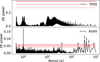 |
Fig. 1 GLS periodograms of photometric TESS (upper panel) and ASAS (lower panel) data, including 0.1, 0.01, and 0.001 FAP levels in red. Significant peaks with periods higher than the 1 d sampling peak are highlighted in cyan triangles. |
5.1.2 Spectroscopic rotation period
To confirm the rotation period around 39 d with spectroscopic indices, we computed their GLS periodograms. In several indicators the long-term trend over 20 years is dominating the signal (e.g., Figure A.1). Since our aim is to determine the rotation period, rather than the long-term trend, we need to account for it.
To do so, we subtracted the mean of all points within 600 d of the observation from each data point. This timescale was chosen to be significantly higher than the plausible rotation period so that only long-term activity cycle trends would be filtered out.
Most of the activity indicators, RV, FWHM, BIS, dLW, Hα, Na D1, and Na D2, have a signal close to the 39 d photometric period (Figure 2). Although the FWHM and BIS 39 d peaks do not reach the 0.1 FAP level, they still appear to be noteworthy, as the highest, apart from the 1 d sampling artifact. Some indicators show a peak around 19 d, which would be the first harmonic of the rotation period (cf. Barnes et al. 2024). The peaks at 49 d in the dLW, Na D1, and Na D2 are unlikely to be aliases of the 39 d signal, as their amplitudes do not match the alias pattern expected from the sampling (Dawson & Fabrycky 2010). Their consistently weaker power across most indicators argues against a rotational origin, but an activity-related explanation cannot be excluded.
In the new RedDots observing campaign in 2021, the star showed strong activity in multiple activity indicators (e.g., differential line width, dLW, Na D1 ) as well as in the RV itself (Fig. 3). A long-term trend, attributable to an activity cycle, can be seen in those indicators (Fig. A.1).
In one of the consecutively observed seasons, the star shows an activity outbreak (Figure 3). The activity is most prominent in the RVs, Na D1, and dLW. In these indicators, two clear minima and maxima separated by 39 d, respectively, can be seen; these suggest increased stellar activity. This is additional evidence for a 39 d rotation period with 19 d as its harmonic. Nevertheless, in the GP models we investigate whether a rotation period around 39 d is still valid when taking the planet signals into account.
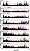 |
Fig. 2 GLS periodograms of HARPS RV data and seven activity indicators described in the plots including 0.1, 0.01, and 0.001 FAP levels. The long-term trend was removed from all time series by subtracting the 600 d average from each observation. The blue line indicates the rotation period determined by photometry. The cyan lines represent signals that we attribute to planets (solid) and candidates (dashed). |
5.2 RV signal search
In this section, we seek to determine the significance of signals in the RVs. Figure 4 shows the GLS periodogram of all HARPS and ESPRESSO RVs. The strongest peak belongs to planet b at 9.3 d with a false alarm probability (FAP) of the signal of 5.8 × 10⁻⁸.
Thus, at this point, we removed the signal from the data. We modeled the new signal with a Keplerian in order to determine the component to subtract. Subtracting the 9.3 d signal leaves the highest peak at 21.8 d with a FAP of 8.0 × 10⁻⁹, which belongs to planet c. Subtracting this signal leaves the 39 d rotation period as the highest peak with an FAP of 3.9 × 10⁻¹². As we shown in the previous section, this belongs to the rotation period; however, for the time being, we chose to remove the signal with a Keplerian. This leaves a signal at 50.7 d with an FAP of 1.6 × 10⁻⁶ at the period of the planet candidate d. Subtracting this 50.7 d signal leaves a peak at 19 d, which is half the rotation period and therefore unlikely to be caused by a planet. To avoid this effect we fitted the stellar activity with a quasiperiodic GP described in 4.2. We fit the hyperparameters simultaneous with the planets and remove the predictive mean. The model with three planets and a GP reveals a signal at 4.4 d with a FAP of 4.6 × 10⁻¹¹ in the residuals. Including the fourth Keplerian signal in the model leaves a signal at 2.2 d with an FAP of 8.3 × 10⁻³. Including this planet in the model as well leaves no significant signals. The highest remaining peak with FAP 3.6 × 10⁻² is at 1.4 d.
We also computed an ℓ1−periodogram (Fig. 5) for the HARPS RVs. With this periodogram, we can model the noise with a combination of a white noise jitter term and a red noise Gaussian term with given correlation length. Then we divide the observations into a 60% training and a 40% test set following the method of Hara et al. (2020). We generated a model, including all Keplerian signals with an FAP<0.1, and a noise term generated with given hyperparameters for white and red noise, on the training set. We then computed the likelihood of the data for the calculated model. For each set of hyperparameters we repeated this procedure 400 times and take the median of the likelihoods. Thus we assigned a likelihood to each set of hyperparameters. By exploring the parameter space for different hyperparameters and looking for the maximum likelihood, we obtained a good model for red and white noise.
We report the FAP values corresponding to the mean in log10 FAP of the best 20% ranked models. For these best parameter sets, 5 peaks in the ℓ1−periodogram remain significant, four of which belong to the periods of the planet candidates at 4.42 d (FAP: 2.6 × 10⁻⁴), 9.26 d (FAP: 1.4 × 10⁻¹⁰), 21.7 d (FAP: 2.0 × 10⁻¹⁰) and 50.7 d (FAP: 5.2 × 10⁻³); the fifth belongs to the rotation period at 39.2 d (FAP: 1.1 × 10⁻³).
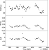 |
Fig. 3 Time series of the active phase of GJ 887 in the RV and in Na D1 and dLW indicators. The spectra were recorded during the 2019 RedDots observing campaign. |
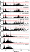 |
Fig. 4 GLS periodogram of RVs 0.1, 0.01 and 0.001 FAP levels, shown in red. The blue line indicates the rotation period determined by photometry and spectroscopy. The cyan lines represent signals that we attribute to planets (solid) and candidates (dashed). The individual panels represent residuals of the respective model in the legend. |
5.3 Modeling of RVs
To determine the number of planets and estimate their orbital parameters, we ran Keplerian models. In the data used in Jeffers et al. (2020), the stellar contribution was minimal that models including and excluding a GP showed similar likelihoods. In the new RVs, however, GJ 887 shows strong activity. Since we have strong evidence for a rotation period around 39 d we can include rotationally modulated GPs. We tried the QP, SHO, and dSHO kernels for the GP models. The SHO failed to faithfully model the activity, yielding a worse log Z and values in the characteristic oscillator frequency that correspond to periods of only a few days with uncertainty on the order of days. These values contradict the spectroscopic and photometric rotation periods and indicate overfitting, as the GP attempts to absorb short-term variability in the RVs. This shows that the SHO kernel does not provide an adequate description of the stellar activity. Models with the QP kernel showed slightly better log Z compared to the dSHO kernel despite being less complex (four parameters rather than five). We adopt wide log-uniform priors on the GP period (J(10,100)) to show that the estimated rotation period from photometry and spectroscopic indices agrees with the GP model. The other GP parameters are taken log-uniform distributions as well and can be found in Table A.2. The priors on the planetary periods were centered on the candidate signals reported by Jeffers et al. (2020) and those identified in our GLS and ℓ1 periodograms. This is common practice for Bayesian model comparison (Gorrini et al. 2023; Dreizler et al. 2024; Basant et al. 2025) as shallow signals can be difficult to find for the algorithm in the presence of multiple planets and red and white noise in the RVs. We could make the argument that to assess the significance of a signal, a prior over the whole parameter space of the period (e.g., J(0.5, 10 000) d) must be considered. Therefore, we additionally report a corrected value for ∆ log Z, where the evidence of a model is multiplied by
 (2)
(2)
for the narrow period range of [P1, P2]. For the other planet parameters, we used uniform priors on the RV amplitude U(0.01,5) since signals of higher order of magnitude would be clearly visible by eye. The eccentricity is fixed to zero in circular models and has a prior of U(0,0.9) in eccentric models as higher eccentricities are very unlikely. The prior for ω is U(0,2π) and t0 has a uniform prior with a width that matches the corresponding period. An extensive overview of all prior is given in Table A.2.
As a first step we tried to fit the two-planet model proposed Jeffers et al. (2020); Harada et al. (2025). Both planets could be recovered clearly ( and
and  on orbits
  and
and  ) on eccentric orbits and the model is overwhelmingly preferred over a model without planets with ∆ log Z = 48.64 (∆ log Z = 34.32 when correcting for the choice of narrow priors). It is also moderately preferred over a model with both or one of the planets on a circular orbit. All Bayesian evidences are summarized in Table A.5. The key models are given capital letters in the text, and are listed in Table 2.
We compare the two-planet model (model A) with a three-planet model, including the 50 d (model B) candidate and retrieve a model with a better evidence by ∆ log Z = 7.25 (∆ log Z = 0.34 when correcting for the choice of narrow priors). For this planet, it is important to note that the GP affects and mitigates the signal. Comparing model A and model B for a non-GP model yields ∆ log Z = 19.20 for the uncorrected and ∆ log Z = 12.29 for the corrected case. Since the candidate was already identified in Jeffers et al. (2020), we named the candidate GJ 887 d. The planet in this case was fitted on a circular orbit, which led to a better d log Z than an eccentric orbit and its resulting RV semi amplitude was  . In both models, the rotation period of the star was around 39 d.
In the residuals of model B, a periodogram peak at 4.4 d appears with a FAP of 7 × 10⁻¹² (Fig. 4 panel 6). This signal was detectable in the raw data (Fig. 4 panel 1 and Fig. 5); however, the peak in the GLS periodogram was less significant than peaks attributed to aliases or noise. Fitting a three-planet model with the candidate at 4.4 d and planets from model A (4.4 d + A = model C) results in a significant improvement of ∆ log Z = 27.15 (∆ log Z = 18.22 with corrected evidences) over A, which is strong evidence for the detection of a new planet. For this and all of the following models, the Bayesian evidences show values where variations of the ∆ log Z values would qualitatively affect the interpretations on statistical significances. Therefore, we ran each model five times and reported the median log Z and its uncertainty according to Nelson et al. (2020). The medians and uncertainties can be found in Table 2. We call this new planet candidate GJ 887 e and it has an amplitude of  . We add the 50 d candidate to model C (C + 50 d = model D) and find an improvement of ∆ log Z = 6.48 (∆ log Z = −0.43) over model C, . The uncertainties of the evidences are both below 1. An overview of all posterior medians and confidence intervals of this model can be found in Table 3.
We computed a GLS periodogram of the residuals of model D to see if any periodic signals remain after subtracting the model. As can be seen in Figure 4 panel 7 another peak has appeared and reached a FAP of 0.0083 in the residuals. The period of this signal is very close to a 2:1 resonance with the 4.4 d planet, but it becomes significant only after removing the signal of the 4.4 d planet. Adding this candidate on an orbit with an eccentricity fixed at 0 to model D (2.2 d + D = model E) leads to an improvement in evidence of ∆ log Z = 4.42 (∆ log Z = −3.27 for the corrected evidences). The uncertainty on log Z is ~1 for both models, which does not change much on the interpretation of the evidences. Allowing for an eccentricity in this model leads to a lower Bayesian evidence. We call this candidate GJ 887 f. The additional signal is fitted with a RV semi-amplitude of  , namely, this is a 4.5σ detection. The ratio between the posterior periods of candidates e and f in the five-planet model is 1.99626
 :1.
:1.
An eccentric planet whose RV signal mimics the RV signal of a resonant pair (Anglada-Escudé et al. 2010) cannot be ruled out easily. A five-planet model with 2.2 d and 4.4 d planets on circular orbits is preferred by ∆ log Z = 5.93 over an otherwise identical four-planet model (4.4 d, 9.3 d, 21.8 d and 50.8 d) with eccentric orbits for the inner three planets. We also note that the evidence for the five-planet model E is a strong improvement over a four-planet model that does not include the 50 d planet (E - 50 d = model F). The Bayesian evidence of model E over model F is ∆ log Z = 9.42 (∆ log Z = 2.51). Posterior medians and confidence intervals of the five-planet model can be found in Table A.6.
Since the addition of candidate f did not lead to an increase in evidence of ∆ log Z > 5 over the model not including the signal, we report the four-planet model D as our preferred model (Table 3). Figure 6 shows the phase folded RV curves. The left panels are phase plots of the whole model: the fit is excellent with few residuals. To assess the impact of the GP, we consider the right panels, which display the phase plots without subtracting the GP model from the RVs. All of the signals are recognizable in the binned phase plots; however, the RVs deviate significantly from the model. This shows that a GP is needed to account for stellar activity in order to detect the low-amplitude signals at 4.4 d and 2.2 d as the evidence for this signal only becomes significant for the GP model. The full GP model is given in Figure A.7. The posterior distributions including correlation plots can be seen in Figure A.4 for the planet parameters, Figure A.5 for jitter and offset parameters, and Figure A.6 for GP parameters.
The planet parameters are all distributed as Gaussians, except for the arguments of periastron, ω, for both eccentric planets. These show roughly uniform posteriors over the whole parameter space. The choice of an alternative parametrization with  and
and  instead of e and ω led to wider confidence intervals of the derived eccentricity and the overall Bayesian evidence was slightly worse so that we retained the standard parametrization of e and ω.
The distributions of the jitters of HARPSpost and HARPSpw sets peak at 0 ms−1. Other than that all parameters have distributions as expected. The α parameter seems to peak at 0, but this happens only due to the fact that we allowed the model to have high α parameters and, thus, a short correlation length. The distribution is expected to peak close to 0 in a linearly scaled plot.
The combination of a long observational base-line and dense sampling yields a high frequency resolution, so we could select very narrow priors for the periods of the inner planets. However, to test that the low-amplitude signals for candidates e and f are not dependent on the narrow priors, we re-ran models D and E with wider priors for the periods of the shallow signals. In model D, the prior of the period of candidate e (f) was U(4.42,4.43) d (U(2.21, 2.22) d), namely, the prior spans 0.01 d. The recovered posterior period was  (
( ), so the 1σ confidence interval is only 2.6% (2.0%) of the prior. Widening the prior by a factor of 10 (15) to U(4.4,4.5) d (U(2.15,2.3) d) yields essentially the same posterior period:
  (
( ). The posteriors are not significantly affected by the prior choice.
To confirm that the results for the planet configurations and parameters do not depend on the activity model, we ran all models with a dSHO kernel. The overall results are similar to the QP models: the rotation period was around 39 d and the planet parameters agree within 1-2σ. Additionally, the models including the 4.4 d planet perform much better than those that do not. There is moderate evidence for the 2.2 d candidate, as there was in the QP model. In the dSHO models however, the evidence for the 50 d planet decreases as the difference between Bayesian evidence between models CdSHO and DdSHO is only ∆ log Z = 6.05. When including the 2.2 d planet the difference between the models is ∆ log Z = 3.31 (EdSHO over FdSHO). This could be because the dSHO model has more parameters and is therefore more flexible. The 50 d signal could be partly absorbed by the GP, which is an effect that happens more efficiently with a more flexible model. The Bayesian evidences of all models we ran are shown in Table A.5.
For the posteriors of the models D and E we tested the (re-sampled) posterior configurations for stability with SPOCK. Some of the samples with higher eccentricities of planets b and c were down-weighted, however, neither of the median values of the posterior distributions was changed significantly by factoring in the stability. The adjusted medians and confidence intervals of the weighted posteriors are tabulated in Tables 3 and A.6.
We also computed the mutual Hill separation (Weiss et al. 2018), with the separation in units of mutual Hill radii,
 (3)
(3)
for neighboring pairs of planets j and j + 1 with the semimajor axes, a, the masses, m, and the host star mass, M. For the five-planet configuration febcd in this system we obtain mutual Hill separations of  (fe),
(fe),  (eb),
(eb),  (bc), and
  (cd). For other planet configurations these separations vary only insignificantly. These values are typical for multiplanet systems (Weiss et al. 2018).
To further examine the short period signals we re-ran models A-F with the unbinned data. This could allow a better representation of the RV signals. The evidence for model E over model D however, was only ∆ log Z = 1.78 (∆ log Z = −5.91 corrected), which could be evidence against the 2.2 d candidate compared to the QP model, but it could also be the effect of short-term activity, which is the reason the data were binned in the first place.
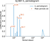 |
Fig. 5 ℓ1-periodogram of all HARPS data. The model includes a white and a red noise model corresponding to the best likelihood as well as all signals exceeding a FAP of 0.1. Those signals are highlighted with red dots and their period. |
log Z values of the results of all referenced GP models with the quasiperiodic (QP) kernel on binned dataa.
Table of posterior medians and 1σ-intervals of model Da.
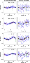 |
Fig. 6 Phase folded plot of a four-planet model including candidates e, b, c, and d. The colors represent HARPSpre (purple), HARPSpost (blue), HARPSpw (green), and ESPRESSO (red) observations. In the left panels the model except for the respective planet component was subtracted from the RVs. In the right panels the model except for the planet and GP components are subtracted from the RVs. The yellow dots indicate phase-binned RV. |
5.4 Injection-recovery tests
To show that planet signals can be recovered and confirmed by Bayesian model comparison as it is used in Section 5.3 in the GP models, we run injection-recovery tests similar to those of Rajpaul et al. (2024). We are particularly interested in the recovery of low-amplitude short-period signals similar to the candidates e and f and periods above the rotation period similar to candidate d. Therefore, we added sinusoidal signals on the original RVs. We selected periods similar to the previously mentioned candidates in regions of the periodogram that show no other significant peaks so that the injected signals are not confused with potential additional signals in the data. We selected the periods 3.1 d as short-period injection and 66 d as long-period injection and injected two different RV semi-amplitude signals in each of these periods. As semi-amplitudes for the short-period signal we used Kinj = 0.94 ms−1 and Kinj = 0.37 ms−1 just as the recovered signals from the candidates e and f. For the long-period signal we injected Kinj = 1.8 m s−1, as recovered for candidate d, and to test the capability of the model, we injected Kinj = 1.2 ms−1 at the same period. With this procedure we created four new time series and for each of these we ran a four-planet model (D) and a five-planet model with a prior including the period of the injected signal (D + injected signal). We then compared the Bayesian evidence of these two models for each time series to determine if the recovery was successful. The widths of the (uniform) priors of the injected planets were similar to the corresponding planets f, e, and d and are tabulated in Table A.4.
For the short-period signal we recovered the Kinj = 0.94 ms−1 with ∆logZ = 29.20, which is a clear detection and the results are similar to the detection of candidate e. The recovered amplitude was  . For the injected Kinj = 0.37 ms−1 the five-planet model performs better than the four-planet model by ∆ log Z = 5.19 and the recovered amplitude was
  . This suggests a strong detection. The difference in Bayesian evidence is comparable to the difference we saw between the four-planet and five-planet models in the original data. That parallel shows the model comparison is behaving consistently: it reacts the same way both to the injected signal we know is real and to the 2.2 d candidate in the actual data. We note that the recovered period of the injected planet was
  which is significantly different from the injected Pinj = 3.1 d, which is a sampling effect caused by timing of observing periods as one large chunk of observations was recorded in 2005 and another large chunk was recorded in 2019, which leads to a sampling frequency of
  which is consistent with the aliasing pattern. Similar patterns can be observed when zooming in on the periods of the other signals, which can be seen in Figure A.8. For this experiment it does not play a role as we were interested in the Bayesian model comparison of the models.
For the long-period injection we were able to recover the injected planet with Kinj = 1.8 m/s with an evidence ∆logZ = 11.53 and a recovered amplitude of  , however, for the Kinj = 1.2 m/s signal, we only recovered the signal with an evidence of ∆ log Z = 1.67 with an amplitude of
  over the four-planet model. This shows that a GP can interfere with planet signals close to the period of the GP.
In conclusion, in the idealized conditions of a circular orbit, with no dynamical interaction with other planets, and in a low noise region of the GLS periodogram, the signal could just be detected. For the candidate f whose orbit could be eccentric or affected by dynamical interactions over time this implies a detection of a planet with the recovered parameters is within reach, but it is on the edge of detectability with the current data. The Bayesian model comparison values for the injected signals match those obtained for the real planets and candidates when using similar priors, which validates our method of using narrow priors.
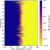 |
Fig. 7 FAP of injected signal with given period and amplitude. The red dashed line describes the smoothed 0.01 FAP level. |
5.5 Detection limits
We can describe detection limits in a more formal way with the methodology of Liebing et al. (2024). The estimation of the detection limit works under the assumption that no signals are present in the residuals and only noise remains. Because the 2.2 d signal remains in the four-planet model residuals, we use the five-planet model residuals. We add a Keplerian signal of a noneccentric planet to the RV residuals of the five-planet GP model. Then we use the FAP calculated by the GLS implementation from Zechmeister & Kürster (2009) at the true, injected period to determine the detectability of the signal. This is done for a grid of amplitudes K and periods P. Our grid spans 0.5100 d with a step size of 0.1 d and 0.1-1 m s−1 with a step size of 0.01 m s−1. We determine the detection threshold using the value of K below which the signal has FAP > 0.01. Figure 7 shows the FAP values over the amplitude-period grid. The red dashed line is the threshold, smoothed by a Savitzky-Golay filter. The mean detection limit over 0.5-100 d is 25 ± 3 cm s−1. For shortperiod signals around 2 d the estimated detection limit is around 23 cm s−1, which would allow the detection of a 37 cm s−1 signal, such as candidate GJ 887 f. For longer periods (>20 d) the detection limit increases to ~26 cm s−1. However, as shown in the previous section, injected signals interact with the GP and the residuals are affected by the GP.
5.6 Coherence of signals
To test whether the candidate planet signals are coherent, we computed sBGLS periodograms for the relevant period ranges. The sBGLS tracks how the significance of a periodicity evolves as data are added sequentially, enabling incoherent activity-induced signals to be distinguished from stable planetary ones. For the stronger signals of planets b, c, d, and the stellar rotation period, we pre-whiten the data by removing all planetary signals and the rotation period as a Keplerian, except for the one being tested. For the signals of candidates f and e we use the residuals of the GP models including planets b, c and d (and e for the periodogram of planet f).
In Figure A.8, we see clearly coherent signals for the candidates f, e, and b. For candidates c and d the signal is most evident in the end of observations, which is characteristic for a coherent signal, however both signals peak around 150-170 and drop off before peaking in the end. This first peak appears for both signals approximately at the time where the star becomes active. Consequently the RVs are dominated by the stellar activity there and interfere with the signals of the candidates. In the end when the activity drops becomes weaker according to the indicators, the candidate signals become stronger again. For the rotation period at 39 d the signal appears coherent at first sight. However, a closer look reveals a drop-off for the last observations. This happens, because the star becomes less active at this period of time.
As a second approach, we investigated in the same RV residuals as described for sBGLS, the temporal stability of the detected periodicities using apodised signals models (Gregory 2016; Hara et al. 2022), which introduce a Gaussian envelope to track how the signal amplitude evolves over time. This technique, employed by Suárez Mascareño et al. (2025) to validate the coherence of planetary signals, enables us to distinguish genuinely stable, planet-like periodicities from activity-induced signals. As test periods we used posterior medians as fixed values from Table A.6. The parameters of the Gaussian from Suárez Mascareño et al. (2025) and remaining planet parameters are fitted using MCMC. All planets and candidates have an amplitude that is stable in the median and within 1 and 2 σ intervals (Figure 8). Only for candidate f the 3 σ confidence interval, shows a stronger signal around 2], 457 000 BJD. We note that the amplitude of the signal discussed here is not necessarily equal to the amplitudes inferred from the GP models. In this analysis, each signal is fitted individually after removing the contributions of other planets and stellar activity, following the procedure described in the sBGLS analysis. The rotation period in contrast shows a signal that is very strong around around 2 459 000 BJD despite not being present at all in the median before that. This shows that the signal of the rotation period at 38.7 d is incoherent.
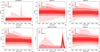 |
Fig. 8 Stability test with apodised models for the candidate signals, showing the evolution of the effective semi-amplitude over the observational baseline. |
5.7 Transit search
Jeffers et al. (2020) detected no planet transits in TESS Sector 2. With two additional TESS Sectors (28 and 69) we revisited this question, searching for transits of the planets and candidates we found in the RVs. We flattened the light curves using splines with a window length of 1 d from the Wōtan package (Hippke et al. 2019) (upper three panels of A.3). To find potential transits we applied the TLS algorithm. In the lower panel of Figure A.3 we can see the SDE of the combined light curve. None of the peaks are significant; no peaks coincide with the RV periods. We can estimate the radius of the planets from their minimum masses from probabilistic models of Chen & Kipping (2017). The radii Rf = 0.81 R⊕, Re = 1.12 R⊕, Rb = 1.77 R⊕, Rc = 2.39 R⊕, and Rd = 2.29 R⊕ combined with the stellar radius of Rs = 0.468 R⊕ predict transit depths of Df = 0.00025, De = 0.00048, Db = 0.00120, Dc = 0.00219, and Dd = 0.00201. The median error of the normalized TESS flux is 0.00011 so that transits of each candidate would be detectable. Although the limited temporal coverage of TESS leaves open the possibility of missed events, no transit signatures are detected in the light curves. The inner planets are therefore non-transiting, and, given both the absence of signals and the lower geometric transit probability of outer planets, it is unlikely that the outer planets transit.
6 Discussion
We determined the rotation period of this important nearby star, and significantly improved the RV analysis. We find strong evidence for planet GJ 887 d in the HZ. We discuss our results below.
6.1 Rotation period
Jeffers et al. (2020) suggested rotation periods of around 37 d and 55 d, but their study was hampered because the star was inactive during their observations. Our new data include coverage during a time when GJ 887 was more active.
We estimated the rotation period of GJ 887 in Section 5.1. ASAS photometry hints at a period around 39 d. Several activity indicators: FWHM, BIS, dLW, Hα, Na D1, and Na D2, as well as the RVs also reveal a 39 d periodicity. In dLW, Hα, Na D1, and Na D2, we see a weaker signal at 49 d; however, since it does not show up in photometry and several indicators it is unlikely to be the rotation period.
In 2019 many spectra were obtained on consecutive nights, and cover a strong activity outbreak. Measuring times between the peaks in the time series yields 39 d for the RV, dLW, and Na D1 time series. In the analysis using apodised models the signal shows a strong amplitude of several ms−1 so that the signal is incoherent and therefore not a planet. Lastly, all GP models with high Bayesian evidence suggest a rotation period around 39 d. Our preferred model, the four-planet model, model D, suggests a rotation period of  when searching with a wide prior of J(10,100). When modeling the rotation period with a Keplerian, residuals appear at Prot/2, which is typical for the rotation period. The signal around 50 d which Jeffers et al. (2020) attributed to either stellar activity or a planet, we now interpret as a planet.
6.2 Assessment of signals in RVs
We found multiple significant signals in the GLS periodograms when subtracting significant signals iteratively at periods 9 d, 21 d, 50 d, 4.4 d, and 2.2 d.
The strongest signals are at 9 d and 21 d and belong to the previously reported planets b and c (Jeffers et al. 2020). The FAPs in the GLS periodograms are 5.8 × 10⁻⁸ and 8.0 × 10⁻⁹ and respectively 1.4 × 10⁻¹⁰ and 2.0 × 10⁻¹⁰ in the l1 periodogram. Fitting both signals in Bayesian models treating the stellar rotation as GP improves the Bayesian evidence by ∆ log Z = 34.56 and ∆ log Z = 14.08. Correcting the evidences for the choice of a narrow prior still leaves strong evidences for both signals (∆ log Z = 26.82 and ∆ log Z = 7.50). The 9 d signal is perfectly coherent in the sBGLS periodogram. The 21 d signal does not appear perfectly coherent, however the incoherence appears in the active phase of the star, where the RV signal is dominated by stellar activity. The amplitude of the signal appears stable over the complete time series according to analysis using apodised models. Consequently, we reported both signals as planets, in agreement with Jeffers et al. (2020).
The signal at 50 d shows a FAP of 1.6 × 10⁻⁶ in the GLS periodogram after subtracting planets b and c and the rotation period with Keplerians and FAP of 5.2 × 10⁻³ in the l1 periodogram. Including the 50 d planet in GP models improves the evidence in all models with ∆ log Z = 6.48 when not fitting the 2.2 d signal and by ∆ log Z = 9.57 when including the signal in the model. When correcting for the choice of a narrow prior of the periods, this evidence decreases to ∆ log Z = −0.43 and ∆ log Z = 2.51, thereby offering only moderate evidence for the signal at best. Using the corrected evidence for the 50 d signal from the non-GP models, we obtained strong evidence for the existence of the planet (∆ log Z = 12.29).
In the four-planet GP model, we reached a 4.6σ detection considering the semi-amplitude and its uncertainty ( ). The signal is consequently significant. The signal shows a similar pattern in the sBGLS periodogram as the confirmed 21 d planet. The amplitude of the planet remains stable for the whole time series using apodised models. The Na D indicators and the dLW show activity at a period of 48 d, however, most of the indicators do not show signals around 50 d. Additionally, the semi-amplitude of the signal in the posterior remains stable independent of how the stellar activity is dealt with. Therefore, we conclude that the signal is most likely caused by a planet and we confirm the signal as planet d.
The signal at 4.4 d is not significant when treating stellar activity with a Keplerian. However, it shows a FAP of 4.6 × 10⁻¹¹ in the residuals of the three-planet GP model. In the ℓ1 periodogram the signal is detected with a FAP of 2.6 × 10⁻⁴. Including the planet in a GP model improves the Bayesian evidence by ∆ log Z = 27.15 (∆ log Z = 18.22 for corrected evidences) compared to the three planet model. The uncertainty on the semiamplitude  suggests a 9.8σ detection. There is no signal at this period in the activity indicators and the signal is coherent in the sBGLS periodogram. The analysis using apodised models shows a constant period over the whole period of observations. Consequently, this is a clear detection of a new planet that we call GJ 887 e.
The signal of the 2.2 d candidate is neither significant in the ℓ1-periodogram nor in the GLS periodogram without subtracting a GP model. However, when subtracting the four-planet GP model including the planets confirmed above, the residuals show a signal with a FAP of 8.3 × 10⁻³ at 2.2 d. Adding the 2.2 d signal improves the fit by ∆ log Z = 4.42 compared to the four-planet model, however, when correcting the evidence for the choice of prior the evidence results in a negative Bayes evidence (∆ log Z = −3.27). In the five-planet model, the signal yields a 4.5 σ detection of the semi-amplitude,  . According to common standards a model needs to show a significance of ∆ log Z > 5 for being considered a planet, which was not achieved in this model. Still, with additional RVs from an ultra-precise instrument such as ESPRESSO, confirmation could be possible if the signal is indeed planetary in origin. Activity plays no role on the timescale of the signal for this star and the signal is coherent in the sBGLS periodogram and in the analysis using apodised models. An alternative explanation is that the signal arises from dynamical interactions with other planets, leaving a residual from the 4.4 d planet. This is plausible since the 2.2 d feature lies close to a mean-motion resonance with planet e. The posterior distribution of the resonant angle φ = 2λ2 - λ1 is strongly clustered (resultant length R = 0.84), peaking near π∕2 with an approximate dispersion σ ≈ 0.58 rad. This clustering indicates the angle is likely librating rather than circulating, which is suggestive of a 2:1 mean-motion resonance.
Harada et al. (2025) investigated the system using 262 archival HIRES and HARPS RVs. Our dataset, comprising 277 HARPS and 12 ESPRESSO RVs, is bigger and consequently more sensitive. The cited authors used less HARPS data and did not treat the rotation period with a GP model; therefore, the 4.4 d and 50 d planets were not detected in that work.
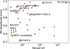 |
Fig. 9 Planets from the NASA Exoplanet Archive with an RV-amplitude below 1.2 m/s that were first discovered with the RV method and that do not have a controversial flag in the archive. The planets are plotted period against RV amplitude. Planets around M stars are highlighted in red and GJ 887 e and f are highlighted in blue and orange. |
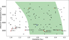 |
Fig. 10 Planets in the NASA Exoplanet Archive with their effective temperatures against their insolation. The HZ (green) according to Kopparapu et al. (2014) for a 5 M⊕ planet. Close-by planets (d < 5 pc) are highlighted in red. GJ 887 d is marked blue. Solar system planets are marked in orange. |
6.3 Detectability of RV signals
To investigate the impact of the GPs on the detectability of planets in our data, we performed injection-recovery tests for long and short period planets. The injected RV signals correspond to the idealized situation of a planet on a circular orbit that does not interact with the other planets, with a period unaffected by aliases or harmonics of other signals.
The injected 66 d signal with the same amplitude as GJ 887 d was easily recovered. However, when decreasing the amplitude to 1.2 ms−1, the signal could no longer be detected. This shows the danger of a GP that acts on a timescale similar to the periods of the planets. A shallow planetary signal can be absorbed or weakened by the GP and can therefore remain undetected.
The short-period planet with Kinj = 0.94 ms−1 could be recovered easily, with a similar improvement in ∆ log Z as planet e. For the Kinj = 0.37 ms−1 injection we obtained a similar evidence as for candidate f, however, the an alias of the injected period was recovered. We conclude that with the current dataset and our model we are not quite able to find strong evidence for a planet of this amplitude at this period.
Figure 9 shows planets that were first detected by RVs. Few planets with K < 1 m s−1 have been detected around M stars: only the recently detected Teegarden’s Star b (Dreizler et al. 2024), Barnard b (González Hernández et al. 2024) and Barnard cde (Basant et al. 2025); both orbit inactive stars. Tee-garden’s Star b was confirmed without a GP model. González Hernández et al. (2024) confirm a short-period signal with a 55 cm s−1 amplitude (Barnard b) and three short-period candidates with amplitudes of 20-47 cm s−1. With more data Basant et al. (2025) confirmed these three candidates modeling stellar activity with a univariate GP, similar to the analysis that has been carried out in this work. GJ 393 b (Amado et al. 2021) has a similar amplitude in a similar orbit to GJ 887 e and was confirmed using a GP. Around K and G stars, a number of sub-meter-per-second (m s−1) detections have been made. Notably, the systems tau Cet (Feng et al. 2017) and HD 215152 Delisle et al. (2018) host multiple planets with sub-m s−1 amplitudes first detected by RVs. All of these systems were observed several hundred times by high-precision spectrographs (e.g., ESPRESSO, HARPS, CARMENES) with a sufficient cadence to sample the periods of the candidates.
Our injection-recovery tests showed that even lower amplitude planets could be found in these short-period orbits with a FAP of 0.01. The detection of planet GJ 887 e and the potential detection of candidate GJ 887 f are part of ongoing progress to detection of lower RV amplitudes. This will help improve our understanding of the properties of low-mass planets.
6.4 Habitability of GJ887d
Planet d with  has instellation of
  using the posteriors of the planetary parameters and the reported Gaussian errors on the stellar parameters (Table 1). The planet is in the HZ (Kopparapu et al. 2014) of its host star (Figure 10). The HZ for GJ 887 spans from planetary orbits of 43 to 122 days. With a minimum mass of
  GJ 887 d is a super-Earth (2 M⊕ < M < 10 M⊕) for inclinations i > 41°. Without an independent radius estimate the density and hence the composition of the planet cannot be determined. According to Luque & Pallé (2022) planets in this mass range have either a rocky, a water-world or a puffy sub-Neptune composition.
In the coming decades an atmospheric characterization of GJ 887 d might be possible with direct imaging missions from space. Due to its brightness and its distance of only 3.29 pc from the Sun, GJ 887 is on the target list of the proposed missions: LIFE (Quanz et al. 2022), the Habitable Exoplanet Observatory (HabEx; Gaudi et al. 2020) and HWO (Mamajek & Stapelfeldt 2024). GJ 887 d could therefore be an ideal target to detect biomarkers on a HZ planet.
For our target planet, we find an angular separation of  and a reflected-light contrast of
  × 10−9, assuming an Earth-like albedo of 0.3. HWO is expected to achieve an inner working angle (IWA) of 65 mas (Tier C) (Mamajek & Stapelfeldt 2024). The mission’s contrast floor is set near (2.5-4) × 10−11 (Mamajek & Stapelfeldt 2024). Thus, the planet’s angular separation from the star is on the edge of the inner working angle making detectability with HWO unclear. Its brightness ratio is orders of magnitude above the HWO detection threshold making the angular separation the dominant limitation.
GJ 887 displays a low level of magnetic activity. Mesquita et al. (2022) estimated GJ887’s HZ to be in Earth-like stellar wind conditions and to receive an Earth-like level of Galactic cosmic rays. However, GJ 887 can nonetheless exhibit some flaring activity (Loyd et al. 2020) which can in principle affect the habitability of GJ 887 d. The interactions of stellar wind, flares, and cosmic rays with GJ 887 d are strongly dependent on the planetary magnetic field, which remains so far unknown.
7 Summary
Our analysis of 277 HARPS and 12 ESPRESSO RVs recovered Jeffers et al. (2020)’s two reported planets. We confirmed a planet in a 50 d orbit within the HZ that was detected by Jeffers et al. (2020). Additionally, we detected and confirmed a planet in a 4.4 d orbit with a sub-m s−1 RV amplitude. A further coherent signal at 2.2 d in the residuals of the four-planet GP model is close to 2:1 resonance with the 4.4 d planet, with an amplitude of  . There is evidence that this signal belongs to a planet; however, the statistical significance is insufficient to claim this signal a planet. The amplitude of the signal is below the stability excursions of the HARPS spectrograph. Future investigations with high-precision spectrographs could help to identify the origin of the signal. Our signal detections were made possible by new RedDots observations with a daily cadence. These were ideal to sample the periods of the planets and captured two rotations of the star, with the period Prot ~ 39 d visible in several activity indicators and the RVs. The same rotation period was found in ASAS photometry and also recovered by the GP modeling of the stellar activity.
GJ 887 is a compelling system for further study. It is a nearby and, hence, bright, M dwarf, hosting a minimum of four planets including a super-Earth-mass, Earth-mass, and potentially subEarth-mass planets. At least one of the planets is in the habitable zone.
Data availability
RV data and activity parameters is also available at the CDS via anonymous ftp to cdsarc.cds.unistra.fr (130.79.128.5) or via https://cdsarc.cds.unistra.fr/viz-bin/cat/J/A+A/707/A93
Acknowledgements
CH and ACC acknowledge support from UKRI/ERC Synergy Grant EP/Z000181/1 (REVEAL). JRB and CAH were funded by the Science and Technology Facilities Council under consolidated grant ST/T000295/1 and ST/X001164/1. FDS acknowledges support from a Marie Curie Action of the European Union (Grant agreement 101030103). We thank the anonymous referee for their careful reading of the manuscript and for their constructive comments, which helped improve the clarity and quality of the paper.
References
- Amado, P. J., Bauer, F. F., Rodríguez López, C., et al. 2021, A&A, 650, A188 [NASA ADS] [CrossRef] [EDP Sciences] [Google Scholar]
- Ambikasaran, S., Foreman-Mackey, D., Greengard, L., Hogg, D. W., & O’Neil, M. 2015, IEEE Trans. Pattern Anal. Mach. Intell., 38, 252 [Google Scholar]
- Anglada-Escudé, G., & Butler, R. P. 2012, ApJS, 200, 15 [Google Scholar]
- Anglada-Escudé, G., López-Morales, M., & Chambers, J. E. 2010, ApJ, 709, 168 [CrossRef] [Google Scholar]
- Anglada-Escudé, G., Amado, P. J., Barnes, J., et al. 2016, Nature, 536, 437 [Google Scholar]
- Barnes, J. R., Jeffers, S. V., Haswell, C. A., et al. 2024, MNRAS, 534, 1257 [NASA ADS] [CrossRef] [Google Scholar]
- Basant, R., Luque, R., Bean, J. L., et al. 2025, ApJ, 982, L1 [Google Scholar]
- Borucki, W. J., Koch, D., Basri, G., et al. 2010, Science, 327, 977 [Google Scholar]
- Boyle, A. W., Mann, A. W., & Bush, J. 2025, ApJ, 985, 233 [Google Scholar]
- Browning, M. K., Basri, G., Marcy, G. W., West, A. A., & Zhang, J. 2010, AJ, 139, 504 [NASA ADS] [CrossRef] [Google Scholar]
- Chen, J., & Kipping, D. 2017, ApJ, 834, 17 [Google Scholar]
- Crass, J., Gaudi, B. S., Leifer, S., et al. 2021, arXiv e-prints [arXiv:2107.14291] [Google Scholar]
- Dawson, R. I., & Fabrycky, D. C. 2010, ApJ, 722, 937 [Google Scholar]
- Delisle, J. B., Ségransan, D., Dumusque, X., et al. 2018, A&A, 614, A133 [NASA ADS] [CrossRef] [EDP Sciences] [Google Scholar]
- Dreizler, S., Jeffers, S. V., Rodríguez, E., et al. 2020, MNRAS, 493, 536 [Google Scholar]
- Dreizler, S., Luque, R., Ribas, I., et al. 2024, A&A, 684, A117 [NASA ADS] [CrossRef] [EDP Sciences] [Google Scholar]
- Dumusque, X., Santos, N. C., Udry, S., Lovis, C., & Bonfils, X. 2011, A&A, 527, A82 [NASA ADS] [CrossRef] [EDP Sciences] [Google Scholar]
- Espinoza, N., Kossakowski, D., & Brahm, R. 2019, MNRAS, 490, 2262 [Google Scholar]
- Feng, F., Tuomi, M., Jones, H. R. A., et al. 2017, AJ, 154, 135 [Google Scholar]
- Foreman-Mackey, D., Agol, E., Ambikasaran, S., & Angus, R. 2017, AJ, 154, 220 [Google Scholar]
- Fulton, B. J., Petigura, E. A., Blunt, S., & Sinukoff, E. 2018, PASP, 130, 044504 [Google Scholar]
- Gaia Collaboration (Vallenari, A., et al.) 2023, A&A, 674, A1 [NASA ADS] [CrossRef] [EDP Sciences] [Google Scholar]
- Gaudi, B. S., Seager, S., Mennesson, B., et al. 2020, arXiv e-prints [arXiv:2001.06683] [Google Scholar]
- González Hernández, J. I., Suárez Mascareño, A., Silva, A. M., et al. 2024, A&A, 690, A79 [NASA ADS] [CrossRef] [EDP Sciences] [Google Scholar]
- Gorrini, P., Astudillo-Defru, N., Dreizler, S., et al. 2022, A&A, 664, A64 [NASA ADS] [CrossRef] [EDP Sciences] [Google Scholar]
- Gorrini, P., Kemmer, J., Dreizler, S., et al. 2023, A&A, 680, A28 [NASA ADS] [CrossRef] [EDP Sciences] [Google Scholar]
- Gregory, P. C. 2016, MNRAS, 458, 2604 [NASA ADS] [CrossRef] [Google Scholar]
- Hara, N. C., Boué, G., Laskar, J., & Correia, A. C. M. 2017, MNRAS, 464, 1220 [Google Scholar]
- Hara, N. C., Bouchy, F., Stalport, M., et al. 2020, A&A, 636, L6 [NASA ADS] [CrossRef] [EDP Sciences] [Google Scholar]
- Hara, N. C., Delisle, J.-B., Unger, N., & Dumusque, X. 2022, A&A, 658, A177 [NASA ADS] [CrossRef] [EDP Sciences] [Google Scholar]
- Harada, C. K., Dressing, C. D., Turtelboom, E. V., et al. 2025, AJ, 170, 343 [Google Scholar]
- Haywood, R. D., Collier Cameron, A., Queloz, D., et al. 2014, MNRAS, 443, 2517 [Google Scholar]
- Hippke, M., & Heller, R. 2019, A&A, 623, A39 [NASA ADS] [CrossRef] [EDP Sciences] [Google Scholar]
- Hippke, M., David, T. J., Mulders, G. D., & Heller, R. 2019, AJ, 158, 143 [Google Scholar]
- Jeffers, S. V., Schöfer, P., Lamert, A., et al. 2018, A&A, 614, A76 [NASA ADS] [CrossRef] [EDP Sciences] [Google Scholar]
- Jeffers, S. V., Dreizler, S., Barnes, J. R., et al. 2020, Science, 368, 1477 [Google Scholar]
- Jeffers, S. V., Barnes, J. R., Schöfer, P., et al. 2022, A&A, 663, A27 [NASA ADS] [CrossRef] [EDP Sciences] [Google Scholar]
- Kopparapu, R. K., Ramirez, R. M., SchottelKotte, J., et al. 2014, ApJ, 787, L29 [Google Scholar]
- Kossakowski, D., Kemmer, J., Bluhm, P., et al. 2021, A&A, 656, A124 [NASA ADS] [CrossRef] [EDP Sciences] [Google Scholar]
- Kovács, G., Zucker, S., & Mazeh, T. 2002, A&A, 391, 369 [Google Scholar]
- Liebing, F., Jeffers, S. V., Gorrini, P., et al. 2024, A&A, 690, A234 [NASA ADS] [CrossRef] [EDP Sciences] [Google Scholar]
- Loyd, R. O. P., Shkolnik, E. L., France, K., Wood, B. E., & Youngblood, A. 2020, RNAAS, 4, 119 [NASA ADS] [Google Scholar]
- Luque, R., & Pallé, E. 2022, Science, 377, 1211 [NASA ADS] [CrossRef] [Google Scholar]
- Mamajek, E., & Stapelfeldt, K. 2024, arXiv e-prints [arXiv:2402.12414] [Google Scholar]
- Mann, A. W., Feiden, G. A., Gaidos, E., Boyajian, T., & von Braun, K. 2015, ApJ, 804, 64 [Google Scholar]
- Mayor, M., Pepe, F., Queloz, D., et al. 2003, The Messenger, 114, 20 [NASA ADS] [Google Scholar]
- Mesquita, A. L., Rodgers-Lee, D., Vidotto, A. A., Atri, D., & Wood, B. E. 2022, MNRAS, 509, 2091 [Google Scholar]
- Mortier, A., & Collier Cameron, A. 2017, A&A, 601, A110 [NASA ADS] [CrossRef] [EDP Sciences] [Google Scholar]
- Nelson, B. E., Ford, E. B., Buchner, J., et al. 2020, AJ, 159, 73 [Google Scholar]
- Newton, E. R., Mondrik, N., Irwin, J., Winters, J. G., & Charbonneau, D. 2018, AJ, 156, 217 [Google Scholar]
- Pepe, F. A., Cristiani, S., Rebolo Lopez, R., et al. 2010, SPIE Conf. Ser., 7735, 77350F [Google Scholar]
- Pojmanski, G. 2002, Acta Astron., 52, 397 [NASA ADS] [Google Scholar]
- Quanz, S. P., Ottiger, M., Fontanet, E., et al. 2022, A&A, 664, A21 [NASA ADS] [CrossRef] [EDP Sciences] [Google Scholar]
- Queloz, D., Henry, G. W., Sivan, J. P., et al. 2001, A&A, 379, 279 [NASA ADS] [CrossRef] [EDP Sciences] [Google Scholar]
- Quirrenbach, A., Amado, P. J., Caballero, J. A., et al. 2014, SPIE Conf. Ser., 9147, 91471F [Google Scholar]
- Rajpaul, V. M., Barragán, O., & Zicher, N. 2024, MNRAS, 530, 4665 [Google Scholar]
- Ricker, G. R., Winn, J. N., Vanderspek, R., et al. 2015, J. Astron. Telesc. Instrum. Syst., 1, 014003 [Google Scholar]
- Robertson, P., & Mahadevan, S. 2014, ApJ, 793, L24 [NASA ADS] [CrossRef] [Google Scholar]
- Speagle, J. S. 2020, MNRAS, 493, 3132 [Google Scholar]
- Suárez Mascareño, A., Rebolo, R., & González Hernández, J. I. 2016, A&A, 595, A12 [Google Scholar]
- Suárez Mascareño, A., Artigau, É., Mignon, L., et al. 2025, A&A, 700, A11 [NASA ADS] [CrossRef] [EDP Sciences] [Google Scholar]
- Tamayo, D., Cranmer, M., Hadden, S., et al. 2020, PNAS, 117, 18194 [CrossRef] [PubMed] [Google Scholar]
- Trotta, R. 2008, Contemp. Phys., 49, 71 [Google Scholar]
- Weiss, L. M., Marcy, G. W., Petigura, E. A., et al. 2018, AJ, 155, 48 [Google Scholar]
- Zechmeister, M., & Kürster, M. 2009, A&A, 496, 577 [CrossRef] [EDP Sciences] [Google Scholar]
- Zechmeister, M., Reiners, A., Amado, P. J., et al. 2018, A&A, 609, A12 [NASA ADS] [CrossRef] [EDP Sciences] [Google Scholar]
Appendix A Supplementary information
Chronological list of observations (before binning) giving PI, number of observations and Program IDa.
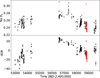 |
Fig. A.1 Long-term trend in Na D1 and dLW indicators over the entire dataset. The phase where the star was active and observed over two full rotations is marked in red |
Priors for all QP models with candidates among f, e, b, c, and da.
First RVs of the HARPS dataset after binning.
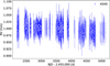 |
Fig. A.2 Photometric time series of GJ 887 from the ASAS survey |
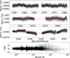 |
Fig. A.3 TESS PDCSAP light curves of GJ 887 of sectors 2, 28, and 69 in the top three panels with trends fitted as splines in red. In the lower panel a Transit Least Squares periodogram is shown along with vertical bars for the location of the planets (solid) and the candidate (dashed). |
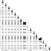 |
Fig. A.4 Correlations between orbital parameters of the planets in the four-planet model including planets e, b, c, and d. |
log Z values of all GP modelsa.
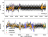 |
Fig. A.7 Four-planet RV model of planets e, b, c, and d including Quasi-periodic GP (black) with 95%-confidence interval (grey) and GP contribution (yellow) |
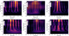 |
Fig. A.8 sBGLS periodograms of all planet candidates and the rotation period of the star. The apparent fringe pattern in all panels is caused by the sampling of the data in two chunks separated by approximately 13 y. |
All Tables
log Z values of the results of all referenced GP models with the quasiperiodic (QP) kernel on binned dataa.
Chronological list of observations (before binning) giving PI, number of observations and Program IDa.
All Figures
|
Fig. 1 GLS periodograms of photometric TESS (upper panel) and ASAS (lower panel) data, including 0.1, 0.01, and 0.001 FAP levels in red. Significant peaks with periods higher than the 1 d sampling peak are highlighted in cyan triangles. |
| In the text | |
|
Fig. 2 GLS periodograms of HARPS RV data and seven activity indicators described in the plots including 0.1, 0.01, and 0.001 FAP levels. The long-term trend was removed from all time series by subtracting the 600 d average from each observation. The blue line indicates the rotation period determined by photometry. The cyan lines represent signals that we attribute to planets (solid) and candidates (dashed). |
| In the text | |
|
Fig. 3 Time series of the active phase of GJ 887 in the RV and in Na D1 and dLW indicators. The spectra were recorded during the 2019 RedDots observing campaign. |
| In the text | |
|
Fig. 4 GLS periodogram of RVs 0.1, 0.01 and 0.001 FAP levels, shown in red. The blue line indicates the rotation period determined by photometry and spectroscopy. The cyan lines represent signals that we attribute to planets (solid) and candidates (dashed). The individual panels represent residuals of the respective model in the legend. |
| In the text | |
|
Fig. 5 ℓ1-periodogram of all HARPS data. The model includes a white and a red noise model corresponding to the best likelihood as well as all signals exceeding a FAP of 0.1. Those signals are highlighted with red dots and their period. |
| In the text | |
|
Fig. 6 Phase folded plot of a four-planet model including candidates e, b, c, and d. The colors represent HARPSpre (purple), HARPSpost (blue), HARPSpw (green), and ESPRESSO (red) observations. In the left panels the model except for the respective planet component was subtracted from the RVs. In the right panels the model except for the planet and GP components are subtracted from the RVs. The yellow dots indicate phase-binned RV. |
| In the text | |
|
Fig. 7 FAP of injected signal with given period and amplitude. The red dashed line describes the smoothed 0.01 FAP level. |
| In the text | |
|
Fig. 8 Stability test with apodised models for the candidate signals, showing the evolution of the effective semi-amplitude over the observational baseline. |
| In the text | |
|
Fig. 9 Planets from the NASA Exoplanet Archive with an RV-amplitude below 1.2 m/s that were first discovered with the RV method and that do not have a controversial flag in the archive. The planets are plotted period against RV amplitude. Planets around M stars are highlighted in red and GJ 887 e and f are highlighted in blue and orange. |
| In the text | |
|
Fig. 10 Planets in the NASA Exoplanet Archive with their effective temperatures against their insolation. The HZ (green) according to Kopparapu et al. (2014) for a 5 M⊕ planet. Close-by planets (d < 5 pc) are highlighted in red. GJ 887 d is marked blue. Solar system planets are marked in orange. |
| In the text | |
|
Fig. A.1 Long-term trend in Na D1 and dLW indicators over the entire dataset. The phase where the star was active and observed over two full rotations is marked in red |
| In the text | |
|
Fig. A.2 Photometric time series of GJ 887 from the ASAS survey |
| In the text | |
|
Fig. A.3 TESS PDCSAP light curves of GJ 887 of sectors 2, 28, and 69 in the top three panels with trends fitted as splines in red. In the lower panel a Transit Least Squares periodogram is shown along with vertical bars for the location of the planets (solid) and the candidate (dashed). |
| In the text | |
|
Fig. A.4 Correlations between orbital parameters of the planets in the four-planet model including planets e, b, c, and d. |
| In the text | |
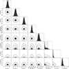 |
Fig. A.5 Same as Fig. A.4, but for jitters and offsets |
| In the text | |
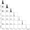 |
Fig. A.6 Same as Fig. A.4, but for the GP parameters. |
| In the text | |
|
Fig. A.7 Four-planet RV model of planets e, b, c, and d including Quasi-periodic GP (black) with 95%-confidence interval (grey) and GP contribution (yellow) |
| In the text | |
|
Fig. A.8 sBGLS periodograms of all planet candidates and the rotation period of the star. The apparent fringe pattern in all panels is caused by the sampling of the data in two chunks separated by approximately 13 y. |
| In the text | |
Current usage metrics show cumulative count of Article Views (full-text article views including HTML views, PDF and ePub downloads, according to the available data) and Abstracts Views on Vision4Press platform.
Data correspond to usage on the plateform after 2015. The current usage metrics is available 48-96 hours after online publication and is updated daily on week days.
Initial download of the metrics may take a while.