| Issue |
A&A
Volume 707, March 2026
|
|
|---|---|---|
| Article Number | A187 | |
| Number of page(s) | 12 | |
| Section | The Sun and the Heliosphere | |
| DOI | https://doi.org/10.1051/0004-6361/202555121 | |
| Published online | 05 March 2026 | |
Convective blueshift inhibition from faculae to small network features
1
Univ. Grenoble Alpes, CNRS, IPAG F-38000 Grenoble, France
2
Université Aix Marseille, CNRS, CNES, LAM Marseille, France
★ Corresponding author: This email address is being protected from spambots. You need JavaScript enabled to view it.
Received:
11
April
2025
Accepted:
5
January
2026
Abstract
Context. Solar granulation properties have long been known to be affected by the presence of a magnetic field, which in turn affects the convective blueshift associated with magnetic regions. Their dependence on magnetic flux is, however, still poorly constrained.
Aims. We studied how the properties of the convective blueshift in faculae and network structures depends on their size and magnetic flux at different positions on the solar disc. We studied the velocity shifts at small (pixel) and intermediate (several granule) spatial scales. Finally, our aim was to validate that simple laws applied to complex structure configurations are sufficient to describe the observed disc-integrated radial velocities in a realistic way.
Methods. We analysed two series of HMI/SDO dopplergrams and magnetograms, which provide insights at different scales, to identify the Doppler shift associated with each structure and its properties. They were then used to evaluate their impact on radial velocity variability.
Results. We confirm the dominant role of the magnetic flux on the Doppler shift and dependence on distance from disc centre. However, we observe a saturation for large magnetic fluxes, as well as an unexpectedly large shift for the smallest network structures compared to that of the larger network structures. This may be due to the small-scale properties of the flows around the flux tubes or to the flux tube properties.
Conclusions. The quiet network strongly contributes to the long-term radial velocity variability, but also exhibits significant rotational modulation. Despite the diversity of properties from network to faculae, simple models to describe the convective blueshift are sufficient to capture the main properties of radial velocity variability in the solar case.
Key words: techniques: spectroscopic / Sun: activity / Sun: granulation
© The Authors 2026
 Open Access article, published by EDP Sciences, under the terms of the Creative Commons Attribution License (https://creativecommons.org/licenses/by/4.0), which permits unrestricted use, distribution, and reproduction in any medium, provided the original work is properly cited.
This article is published in open access under the Subscribe to Open model. This email address is being protected from spambots. You need JavaScript enabled to view it. to support open access publication.
1. Introduction
Granulation properties have been observed to be significantly different in faculae compared to the quiet Sun, which is known as abnormal granulation (e.g. Dunn & Zirker 1973). Smaller granules are observed around spots (e.g. Macris 1979; Schmidt et al. 1988), i.e. in faculae. In addition to a smaller size, their contrast also decreases and they last longer (Title et al. 1988, 1989, 1992; Berger et al. 1998; Narayan & Scharmer 2010). Title et al. (1992) found a sharp edge around active regions, with normal granulation present up to the edge of the active regions. Such properties have been explained by the inhibition of convective flows due to magnetic fields in active regions (Livingston 1982; Miller et al. 1984; Cavallini et al. 1985), leading in turn to an attenuation of the convective blueshift, i.e. a redshift based on the analysis of a limited sample of active regions (Miller et al. 1984; Cavallini et al. 1985; Immerschitt & Schroeter 1989). Magnetohydrodynamics (MHD) simulations of convection in the presence of a magnetic field confirm reduced velocities (Vögler 2005; Beeck et al. 2015), with small impact below 100 G.
Following these earlier works, many studies have been conducted to characterise the intensity properties of abnormal granulation in faculae, but also in the network, since this component is important to consider in order to explain the long-term variability of the solar irradiance (Foukal et al. 1991; Walton et al. 2003; Ermolli et al. 2003; Solanki et al. 2006). These studies have usually focused on limited samples but very high spatial resolution images (such as with HINODE) at the disc centre, on faculae and network (Kobel et al. 2012; Romano et al. 2012), or on pores (Morinaga et al. 2008). In addition, strong downflows around bright points have been observed, and they are stronger in bright points compared to faculae (Ishikawa et al. 2007; Romano et al. 2012). Kostik & Khomenko (2012) studied separately granules and intergranules, confirming lower velocities for high magnetic fields, while strong downflows appear in intergranular lanes.
On the other hand, there have been fewer studies aiming at actually quantifying the attenuation of the flows due to magnetic field. An attenuation of typically two-thirds was found by Brandt & Solanki (1990) in the faculae. Based on the observation of downflows around a pore, Morinaga et al. (2008) concluded that the flows are impacted by the magnetic flux and not by the magnetic field strength, and therefore strongly relate to the filling factor. The strong downflows around magnetic flux tubes were studied in various environments by Buehler et al. (2019) based on very high spatial resolution images, including vector magnetic field maps providing access to the magnetic field strength. Morinaga et al. (2008) and Kobel et al. (2012) found a smaller root mean square (RMS) of the line-of-sight (LOS) velocity for strong magnetic fluxes. Meunier et al. (2010b) analysed a larger set of data, but with a lower spatial resolution based on the Michelson Doppler Imager (MDI) on the Solar and Heliospheric Observatory (SOHO), and found larger redshifts in structures with larger magnetic fluxes and sizes. Most of these studies were performed at disc centre or in a limited range of μ (cosine of the angle between the LOS and the perpendicular to the solar surface). In addition, the analysis of full disc maps from the Helioseismic and Magnetic Imager (HMI) on the Solar Dynamics Observatory (SDO) (Scherrer et al. 2012) by Palumbo et al. (2024b) showed a reversal of the convective blueshift attenuation in faculae and network for μ around 0.4, in agreement with the simulations performed by Cegla et al. (2018). Cegla et al. (2018), Ellwarth et al. (2023), and Palumbo et al. (2024b) provide an estimate of the limb effect for the quiet Sun (Beckers & Nelson 1978; Dravins 1982; Balthasar 1985) respectively with MHD simulations, SDO data, and the solar atlas of the Institut for Astrophysics and Geophysics (IAG) in Göttingen. The limb effect was found to strongly depend on the spectral line, however (Löhner-Böttcher et al. 2018; Stief et al. 2019). Palumbo et al. (2024b) then focused on the difference between faculae, network, and spots, and studied the dispersion in velocity as a function of μ. This dispersion was also studied for different categories of structures by Criscuoli (2013).
For this paper we wanted to study in more detail the properties of the convective blueshift for different types of structures, based on magnetic flux and size, focusing on faculae and network compared to the quiet Sun. This should also provide a better understanding of the contribution of the different types of structures on disc-integrated radial velocity (RV) variability, dominated by the convective blueshift inhibition in faculae for solar-type (F, G, and K) stars (e.g. Saar & Donahue 1997; Meunier et al. 2010a). For this purpose we used time series of HMI/SDO maps, and studied the dependence on the different parameters, both at disc centre and as a function of μ. Reconstructed time series based on those properties were used to quantify the contribution of the different structures, and to compare models and HARPS-N observations, as done in Meunier et al. (2024).
The outline of the paper is as follows. We first present in Sect. 2 why such properties are important to simulate RV time series. We then describe the datasets and data analysis in Sect. 3, providing velocities at different spatial scales within and outside of the magnetic structures. We present in Sect. 4 the results, first focusing on the centre of the disc, and then considering the dependence on μ. We analyse reconstructed time series in Sect. 5. We conclude in Sect. 6.
2. Requirements for simulations
To model the disc-integrated RV, one must average the spatially resolved structures of various kinds weighted with the fraction of surface on which they occur and their brightness. Simulating all these effects is extremely useful for building synthetic time series that are as realistic as possible. They can then be used to design blind tests to perform exoplanet retrieval or characterisation performance (Dumusque 2016; Dumusque et al. 2017; Meunier et al. 2019a; Meunier & Lagrange 2019; Meunier et al. 2020, 2023). In addition, they can also be used to understand better their impact on RV time series, for example the non-linear relationship between RV due to convective blueshift inhibition and chromospheric emission (Meunier et al. 2019b), or the better correlation with the unsigned magnetic flux (Haywood et al. 2022). This better understanding can in turn be useful to improve mitigating procedures. To date, such models have not been used to directly fit RV time series because of the huge number of free parameters it would represent and the poor temporal sampling of usual RV time series (but see Dumusque et al. 2014, for some tests), which is added to the strong degeneracy between parameters and the strong stochasticity of these processes. However, physical properties are necessary to elaborate statistical models that can be applied to observed RVs and help in disentangling activity from planet contributions (Hara & Delisle 2025). Simulations of synthetic RV time series therefore require a good knowledge of many processes acting at different temporal scales:
-
Spot and facula contrast: This effect directly impacts RVs at the rotational modulation, with an amplitude of the signal depending on size and stellar inclination for an individual structure, and varying on cycle timescales. The size distribution of spots and faculae are well known for the Sun (see Borgniet et al. 2015, for use in synthetic time series). Spot contrasts are also well-known for the Sun, while a trend with Teff has been observed for other stars (Berdyugina 2005). The prediction of facula contrasts as a function of spectral type has been performed by Norris et al. (2017), based on MHD simulations. Realistic time series should also take into account other properties such as the latitudinal distribution over the cycle (butterfly diagram) or structure evolution (see Borgniet et al. 2015, and references therein). Many simulations aiming at producing RV synthetic time series based on such properties have been performed for the last two decades (e.g. Desort et al. 2007; Dumusque et al. 2014; Herrero et al. 2016).
-
Attenuation of the convective blueshift in faculae: This effect appears to be dominant in the solar case (e.g. Meunier et al. 2010a). The simulation of this effect requires a similar knowledge to the previous one, but also the amplitude of its attenuation in faculae. This parameter is what we focus on in this paper.
-
Oscillations, granulation and supergranulation: Simulations based on granule properties paving the surface with various approaches have been implemented (Meunier et al. 2015; Cegla et al. 2019; Sulis et al. 2020; Palumbo et al. 2024a), but MHD simulations are very time consuming and require huge storage space. However, the knowledge of the amplitude of their effects as well as their frequency dependence is sufficient to model them, based on laws such as in Harvey (1984) for example. Supergranulation is particularly problematic (Meunier & Lagrange 2019, 2020b) because it has a strong impact, but large-scale MHD simulations are lacking, and no activity indicator has been identified yet.
-
Meridional circulation: This poleward large-scale flow in the case of the Sun varies over the cycle, which leads to a variation in RV when integrated over the whole surface (Makarov 2010; Meunier & Lagrange 2020a). To model its contribution, we need to know the amplitude of the meridional circulation, how it varies over the cycle, and its large-scale configuration (one cell versus multi-cell). The extrapolation to stars other than the Sun has therefore not yet been well established.
For this paper we focused on the inhibition of the convective blueshift in faculae. We studied how fine effects depending on size and magnetic flux across the disc affect synthetic time series.
3. Data and method
3.1. Dataset
We analysed SDO/HMI data obtained on the same days as the three-year HARPS-N solar time series (Dumusque et al. 2021) studied in Meunier et al. (2024), whenever intensity (corrected from centre-to-limb variation), magnetic field, and Doppler maps were available. Two sets were used, both retrieved from the HMI archive: the original maps, available at times close to the average HARPS-N observing time each day, as in Meunier et al. (2024) (hereafter Set 1); magnetic field and Doppler maps after deconvolution which corrects for the instrumental point spread function (PSF), including a small-scale component as well as a large-scale component corresponding to stray light (Couvidat et al. 2016; Criscuoli et al. 2017) (hereafter Set 2). Most of these maps are available at a time slightly different from Set 1. This led to 599 maps for Set 1 and 595 for Set 2. Intensity maps were used to identify spots and remove them from the detailed analysis of LOS velocities that is discussed in Sect. 4. Magnetograms provide the magnetic flux (i.e. integrated over each pixel): They are used to identify magnetic structures and to relate the velocities to magnetic flux at different spatial scales.
3.2. Data analysis
We divided the magnetic flux provided by SDO/HMI by μ, based on the assumption that the magnetic flux tubes are close to vertical in active regions and in the network. A threshold depending on μ was applied in order to take the increasing noise towards the edges into account, i.e. Bth/μ (Yeo et al. 2013). We used Bth values of 24 G for Set 1 (Yeo et al. 2013, the level of 24 G at the centre of the disc corresponding to about 3-σ of the noise level) and 50 G for Set 2, in order to account for the larger values of the magnetic flux in structures and the higher noise level after deconvolution. The sharper images indeed lead to larger fluctuations in the magnetic field and in the granular velocity field, as illustrated in Fig. A.1. This threshold allows us to identify the magnetic structures from which the spots are then eliminated on the basis of the intensity map (see Palumbo et al. 2024b, for results on spots) in order to focus on faculae and network structures. Structures with fewer than 4 pixels are removed to avoid outliers due to noise. In the following, structure sizes are in parts per million (ppm) of the solar hemisphere.
Examples of maps are shown in Fig. 1. A zoomed-in image at disc centre is shown in Fig. 2 for both sets, illustrating the different ranges of structure sizes that are discussed in the following sections: structures below 2 ppm and in the range of 2–20 ppm correspond to the quiet network (in pink in Fig. 2; the quiet Sun outside of any network feature is in white). The smallest structures have a size of ∼0.2 ppm, i.e. the size of a small granule. Structures above 100 ppm are typically in active regions, while intermediate ranges correspond to decaying active regions or active network (Harvey & White 1999). We note that Palumbo et al. (2024b) consider two categories of structures, the network below 20 ppm and the faculae above 20 ppm, so their network categories correspond to the quiet network in the terminology from Harvey & White (1999). The comparison between the maps of Set 1 and 2 shows that after deconvolution the structures are smaller; this will impact the position of the curves in the subsequent analysis. The distributions of structure sizes are compared in Fig. A.2. They also present more complex contours and gaps; with sharper images, the selection of the pixels with magnetic flux eliminates more pixels that were inside granules, which is not the case with Set 1.
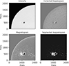 |
Fig. 1. Example of maps (only one-quarter of the field is shown). Shown are the intensity map and the corrected Dopplergram (upper row) and the magnetic flux map and segmented map (lower row), for Set 2. |
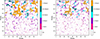 |
Fig. 2. Zoomed-in image at disc centre on a segmented map, illustrating the magnetic structures in different size ranges, for Set 1 (left panel) and Set 2 (right panel). The two maps are separated by 2.5 hours, which distorts the structures only slightly. |
The velocities provided by the Dopplergrams were corrected as in Milbourne et al. (2019) and Haywood et al. (2022), who also used HMI velocities in similar conditions, i.e. from the spacecraft velocities, based on the information given in the headers of the files, and from differential rotation. HMI velocities were computed based on six tuning positions of the filter Schou et al. (2012) and based on a complex calibration procedure. However, the range of velocities covered by the algorithm is [−6.5,+6.5] km/s to account for the spacecraft velocities, solar rotation, and flows (which could be up to several km/s in granulation or spots, for example), which is faster than the flows studied in the present paper. It has been shown that spectral resolution impacts the velocities derived from the position of the spectral line (e.g. de la Cruz Rodríguez et al. 2011). However, Couvidat et al. (2012) compared different algorithms with ground-based observations to test their validity and found a very good agreement, even in the presence of strong magnetic fields, except a possible lack of convergence for very high velocity (above 8.5 km/s) that may appear in certain spot configurations. However, in this paper, we focus on faculae and network structure, and not on spots.
For each set, based on the corrected maps and structure identifications, we computed average velocities V and absolute magnetic fluxes B with three different approaches, described below, as well as their position on the disc. This was done first for each magnetic structure as defined above, but also on 8 × 8 pixel boxes paving the whole surface (including outside faculae and network) in order to characterise locally (while still averaging over several granules) the relation between V and B, as done in previous works on the intensity contrasts (e.g. Kobel et al. 2011, 2012). This size corresponds approximately to a scale of 2.9 Mm at disc centre and ∼2.8 ppm, so that there are a few granules in the box. We identified whether the box includes pixels from a magnetic structure; if there is only one (to avoid ambiguities), we kept the information about that structure, in particular its size and B, as well as the fraction of overlapping. To complete this analysis, we also considered V and B at the pixel scale (i.e. at a scale significantly smaller than a granule), for pixels inside a structure only. In the following, the subscripts struct, box, and pix refer to these three approaches.
In this paper we are interested in the difference between the velocities (in a structure, box, or pixel) from which the quiet-Sun velocity has been subtracted. Velocities in boxes with B lower than 8/μ G are used to build a reference quiet-Sun velocity. The average curves as a function of μ are shown in Fig. B.1 in Appendix B. In practice, the subtraction is made based on a 2D map, built from all such quiet-Sun boxes, to subtract any residual that would remain. This quiet-Sun velocity is then subtracted from all the above velocities, leading to a ΔV, which is studied in the following section. We note that unlike the approach adopted by Palumbo et al. (2024b), the velocities are not weighted by intensities in our analysis.
4. Properties of the convective blueshift inhibition from faculae to network
4.1. Disc centre analysis
We first focus on the relation between ΔV and the magnetic flux at the centre of the disc. Figure 3 shows ΔV as a function of B for the pixel and box approaches for both datasets (before and after deconvolution). We recall that a positive ΔV is a redshift that could correspond to an attenuation of the convective blueshift, and to downflows. As expected, there is a strong dependence on the magnetic flux. However, the relationship is not linear as the slope decreases with increasing magnetic flux in both cases, showing a saturation of the effect. In the case of the pixel approach, there is not much variation above 500 G. Such an effect cannot be due to the way HMI velocities are computed because, as discussed above, the range covered by the instrument is much larger. It is also seen in both sets, so that this is not due to stray light.
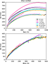 |
Fig. 3. ΔV as a function of average magnetic flux for the pixel approach (upper panel) and the box approach (lower panel) at disc centre (μ > 0.95), for Set 1 (dashed) and Set 2 (solid). The black curve corresponds to points, and the colours to the different structure sizes (of the structure the pixel or the box it belongs to). We note the difference in scales in the two panels. |
The box approach, which averages over several granules, does not exhibit any difference between ΔV curves for different ranges of sizes (of the structure to which the box belongs). The curves are also similar for both sets. This shows that our data are not sensitive to local downflows for example, and the curves represent well the behaviour of the attenuation of the granular flows in granulation in magnetic regions for different fluxes.
On the other hand, the pixel analysis leads to two specific features: overall larger ΔV after deconvolution, and a larger ΔV for the very small network features (< 2 ppm) and to a lesser extent for the 2–20 ppm range, for a given B in the pixel. This difference with pixels belonging to large structures reaches a few 100 m/s for Set 2. This effect is much smaller than the range of velocities in the HMI computation, so we do not expect an effect of this magnitude to be due to the way the velocities are computed. The stray light is not responsible for this effect either, since it is even stronger after deconvolution. The velocity properties, at the scale of the pixel, therefore depend on where the pixel is, even for a given B. Despite the strong effect of B, which appears to be dominant, there are therefore other differences between the network and the faculae. ΔV values are also stronger than can be expected from the attenuation of the convective blueshift (a few 100 m/s). A possible explanation could be the different properties of the flux tubes (while keeping the same magnetic flux) in different environments. However, the inclination of flux tubes, which should impact the convective flows, appears to be very similar in faculae and the network (Buehler et al. 2019), so this cannot be the cause of the observed differences. However, Buehler et al. (2019) found slightly larger flux tubes in network structures compared to active regions, which means they may have a stronger impact on the convective flows. An alternative explanation could be an effect not related to the attenuation of the convective blueshift itself. Very high spatial resolution observations show that stronger downflows, by several km/s, are observed in the network than in the faculae (e.g. Romano et al. 2012). Such flows are not resolved here, but it is likely that they produce such an effect that is more visible after deconvolution.
We note that previous results on the convective blueshift (Meunier et al. 2010b; Palumbo et al. 2024b) found an increase in velocity with increasing structure size. This may be due to the fact that, when considering all structures, the strong correlation between size and average flux dominates the relationship, while there is in fact an underlying behaviour which is quite different when considering a given value of B. We therefore now turn to the properties of ΔV averaged over structures of different sizes. Figure 4 shows ΔV as a function of structure size for different B ranges (upper panel) for the two datasets. First of all, we note that there are offsets between the curves for Sets 1 and 2. This is due to the fact that the magnetic flux and velocity scales are different, and a given structure is smaller when defined with Set 2. This is also responsible for the fact that the yellow B > 200 G curve is shown only for Set 2, while the pink B < 50 G curve is missing (because it is below the threshold). The displacement observed for the large structures is not clear, however, because one might expect a level for both sets that is similar to that for the box analysis. However, it is possible that even for large structures, the segmentation on the data after deconvolution still eliminates some granule centres, leading to a certain impact of the downflows (effects not present in the box analysis).
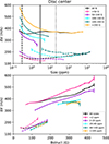 |
Fig. 4. ΔV as a function of average magnetic flux for the structure approach at disc centre (μ > 0.95) vs size for different ranges of B (upper panel) and vs B for different ranges of size (lower panel), for Set 1 (dashed) and Set 2 (solid). The black curves are for all B (all sizes). The vertical black lines correspond to the typical granular size (dashed), the box size (solid), and the 20 ppm scale (network-active region interface, dotted). |
For both sets, however, we find that for a given B, ΔV decreases as the size increases, while the curve considering all B (in black) globally increases (except for very small structures, < 2 ppm) for Set 1 and is flatter for Set 2. The difference between the two black curves may be due to a different B-size relationship, discussed below. On the other hand, ΔV versus B (lower panel) increases for all size categories, but again, for a given B, ΔV is larger for very small structures.
For Set 2, the average ΔV for large regions is a few 100 m/s, which is compatible with a strong attenuation of the convective blueshift. At small scales we observe larger velocity shifts (keeping in mind that positive velocities mean downflows), as for the pixel analysis. It is therefore likely that there is a strong impact of the preferential location of the magnetic network in downflows at those scales.
As mentioned above, it is well known (e.g. Hagenaar et al. 2003; Meunier 2003) that the average flux in structures correlates with the size, as illustrated in the upper panel of Fig. 5 for Set 2. There are also many more small structures compared to the largest ones (see also Parnell et al. 2009; Thornton & Parnell 2011, for the power-law distribution in magnetic flux). When considering a given size, structures with B lower than average (represented in pink, below the orange dots) have a smaller ΔV (middle panel), while those with a larger B (in green) have a larger ΔV. This could be due to the fact that the latter are likely to be more compact structures. A calculation of the perimeter of the structures1 confirms this, as shown by the distribution of the ratio of perimeter to size (lower panel of Fig. 5). More diluted structures should correspond to a later evolutionary state of faculae, such as decaying active regions (Harvey & White 1999; van Driel-Gesztelyi & Green 2015). We expect a strong concentration of flux tubes in compact structures, leading to a stronger magnetic flux, which is consistent with a strong impact of the magnetic flux. In addition, similar plots for Set 1 are shown in Fig. A.3. Although qualitatively similar, we note that the size–magnetic flux relationship is more linear, compared to a trend to saturate above 10 ppm for Set 2. This may be due to the stray light effect, which should affect smaller structures more strongly, because they are more easily contaminated by quiet-Sun values, therefore changing the shape of the curve. This could explain why in Fig. 4 some trends are stronger with Set 1.
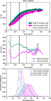 |
Fig. 5. Upper panel: B vs structure size for Set 2. The coloured area show the 1σ dispersion, and the orange dots a polynomial fit on the binned B vs size. Middle panel: ΔV vs size for the two categories of structures, with B larger than the orange curve in green, and with B smaller than the orange curve in magenta. Lower panel: Distribution of the perimeter/size ratio for these two categories of structures. The vertical black lines correspond to the typical granular size (dashed), the box size (solid), and the 20 ppm scale (network-active region interface, dotted). |
We also note that even for weak fields (see e.g. the bottom panel in Fig. 3), ΔV values above 100 m/s are observed. Although it is difficult to clearly separate the convective blueshift and the downflow effect for the magnetic network, they are bound to contribute significantly to RV due to the attenuation of the convective blueshift. However, we do not expect a strong rotational modulation, given that they are spread over the whole surface. As for solar irradiance, for which it is necessary to consider the contribution of the network (Foukal et al. 1991; Walton et al. 2003; Ermolli et al. 2003) to long-term variability, it should then also contribute to long-term radial velocity. This is quantified in Sect. 5.
4.2. Dependence on μ
Figure 6 shows ΔV versus μ for the different approaches. The general behaviour is very similar to that found by Palumbo et al. (2024b), with a sign reversal of ΔV for μ around 0.4. This behaviour is similar for all approaches, and therefore at different spatial scales. The different curves in each panel correspond to different ranges of B, which is the dominant source of variability. We note that for the lowest B ranges, we cannot determine ΔV for very low μ due to the threshold choice (increase in noise away from the centre of the disc). As discussed in Cegla et al. (2018), the sign reversal of ΔV when going towards the limb is likely to be related to the corrugation of the surface due to granulation (Carlsson et al. 2004; Dravins 2008): when observing the photosphere, one does not see the same height in the atmosphere in the granules and intergranules, so it can be visualised as hills and valleys. At the centre of the disc all parts are seen, but very close to the limb some parts of the granules become hidden behind the granule in front of them. We observe a smaller fraction of the downflows; the horizontal flows coming towards us are also hidden, so that the velocities are dominated by the horizontal flows going away from us (i.e. redshift), and hence the sign reversal in ΔV.
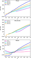 |
Fig. 6. ΔV vs μ for the pixel (upper panel), structure (middle panel), and box (lower panel) approaches, for different categories of B. |
We find that the value of μ at which ΔV reverses sign depends on B. For each approach and range in B, we computed the value of μ corresponding to the sign reversal. The results are shown in Fig. 7 for Set 2: for the structure approach, we observe a decrease in μ for B decreasing down to ∼200 G. The interpretation is not yet clear. One may indeed expect, in the presence of a larger magnetic flux, that the surface is less corrugated so that the sign reversal should appear closer to the limb. There also appears to be an increase in μ towards lower values of B. However, very low values of B away from the disc centre may not be reliable due to the impact of noise.
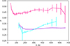 |
Fig. 7. Values of μ for which ΔV changes sign vs B for the three approaches, pixel (violet), structure (cyan), and box (pink), for Set 2. |
Finally, in the previous section focusing on the centre of the disc, we found that for a given B, ΔV was unexpectedly larger for very small structures. Figure 8 illustrates how this difference in ΔV depends on μ. For weak fields, the larger ΔV for small structures is visible close to the centre of the disc only, while it is visible up to lower μ values when B increases. Detailed numerical MHD simulations would be needed to estimate whether this behaviour is more compatible with a stronger convective blueshift in the smallest structures, for example due to larger flux tubes or with the strong downflow interpretation. However, one may expect strong downflows around flux tubes to be much less visible at very low μ, which may favour an interpretation in terms of flux tube properties.
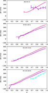 |
Fig. 8. ΔV vs μ for different ranges in B (structure approach), for Set 2, and different ranges in size: < 2 ppm (pink), 2–20 ppm (violet), and > 20 ppm (cyan). |
5. Time series analysis
The objective of this section is to estimate the impact of various categories of structures, from the network to active regions, on RV variability, based on two hypotheses: a simple law for ΔV as in Meunier et al. (2024), and the obtained ΔV values discussed in the previous section. In order to be consistent with the way the image segmentation is performed in Meunier et al. (2024), we used the results obtained with Set 1, which also has the advantage of being on average at the same time as the HARPS-N data.
5.1. Reconstruction of RV time series
We analytically computed the different contributions to RV of all structures at each time, as in the simulations of Meunier et al. (2019a), based on the position (latitude, longitude), size, ΔV, and intensity contrast of all structures. Similar models were used in Meunier et al. (2024) for comparison with HARPS-N observations. The two main differences with the present work are i) instead of using a general prescription for the convective blueshift and the contrast, we use the observed values (ΔV and intensity maps), which allows more diversity between structures, and ii) the threshold used to define the structures is lower here because our objective is to include as much as possible of the magnetic regions, while in Meunier et al. (2024) the goal is to make a comparison with models that were used previously, and therefore the structures had to be defined in a consistent manner.
In the following, we therefore discuss RV due to the convective blueshift in faculae and network (RVconvpl), and in spots (RVconvsp) (the latter was assumed to be negligible in Meunier et al. 2019a), and RV due to the photometric effect in faculae and network (RVphotpl) and in spots (RVphotsp). They are shown in Fig. C.1 in Appendix C. In addition, RVconvsp is also computed separately for the five categories, in sizes studied in the previous section, to study their relative contribution. We note that at this stage the amplitudes of the RV are not yet scaled to the observations, so that their absolute value is not the same as observed RV derived from a large set of spectral lines. This scaling is discussed in Sect. 5.3.
5.2. Contribution of the different size categories to RV variability
We first focus on the convective blueshift in faculae and network, RVconvpl, calculated separately for different size categories and based on the ΔV analyses in Sect. 4. Figure 9 illustrates the long-term variability (smoothed time series over a rotation, upper panel) and the rotational modulation (lower panel). The very small network structures (below 2 ppm) do not contribute significantly to the variability at the rotational and long scales, which can be checked by a Lomb–Scargle periodogram. However, the quiet network in the range of 2–20 ppm contributes to the rotation modulation and to the long-term variability. At the rotation scale, they represent about one-third of the RMS of the largest faculae (> 100 ppm), but they are similar to the signal due to intermediate sizes. A Lomb–Scargle periodogram, not shown here, confirms that all structures above 2 ppm contribute to both the rotational timescale and to long periods. This is in contrast to the results of Milbourne et al. (2019), who argued that the network was negligible. These network structures contribute significantly to long-term variability, as summarised in Table 1 for the two timescales. We note that all structures below 20 ppm (including the very small ones) contribute significantly to the offset in RV (of the order of 1 m/s), since many structures are present over the whole surface at all times.
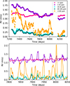 |
Fig. 9. Smoothed time series for the five categories in size (upper panel) and zoomed in on the residuals (lower panel). |
Contribution to RV convective blueshift variability.
5.3. Comparison with simple models and HARPS-N observations
In Meunier et al. (2024) the comparison of the model with HARPS-N RVs (Dumusque et al. 2021) shows a general agreement, after scaling of the convective blueshift prescription, with a correlation of the order of 0.8 between the two time series. We identified the main differences as being due to the following: i) instrumental effects at the level of 2 m/s due to the regular warm-up of the detector; ii) supergranulation, not included in the model, at the level of 0.7–0.9 m/s (Al Moulla et al. 2023; Lakeland et al. 2024); iii) a possible departure from the prescribed simple law for specific active regions, as well as the impact of the convective blueshift inhibition in spots. In this section we focus on this last point and compare the reconstructed RV with all contributions (Sect. 5.1) with the best model in Meunier et al. (2024).
The reconstructed RV we wish to compare with the HARPS-N observations and with the model from Meunier et al. (2024) (hereafter Mod2024) are built as the sum of the different contributions, each multiplied by a factor that is fitted on the observations by minimising the χ2: i) RVconvpl is either considered as a whole (Mod1cat), or split into two categories that are fitted separately (below and above 20 ppm, Mod2cat), or in five categories (as above, Mod5cat); ii) RVconvsp; iii) RVphotpl and RVphotsp are regrouped; iv) an additional trend with time as in Meunier et al. (2024) is also tested; v) a constant offset. Scaling is necessary because ΔV is computed from the Dopplergrams obtained from a single spectral line (Fe line at 6173 Å), while observed RV are obtained from thousands of lines covering a large spectral range (385–691 nm for HARPS for example). In addition, this prescription also strongly depends on how the structures are defined (typically the segmentation threshold applied to magnetograms).
In general, the different options lead to very similar results, as illustrated in Fig. 10, the fit based on all size categories being only slightly better than Mod2024, and the fit based on two categories slightly worse. The multiplying factors are typically in the range 1.1–2.1 for the largest structures contributing to RVconvpl, in the range 1.6–2.0 for RVconvsp, and in the range 1.3–1.4 for RVphotpl+RVphotsp. The correlation between those models and the observations is similar to what was obtained with Mod2024 (Pearson correlation of the order of 0.78, RMS of the RV residual around 0.94 m/s). The correlation between Mod2024 and these models is around 0.95. The new models are slightly better for some of the peaks for which there was a departure for Mod2024 (for example, for around t = 8000), but there is no general improvement. The comparison of the residuals and their periodograms shows that there is only a weak signal remaining corresponding to the rotation modulation (at around half the rotation period), which is furthermore below the 1% false alarm probability level. In addition, there is a small trend for Mod2024 (which we recall was based on a simple law for the convective blueshift inhibition) to be a better match to the observation at the beginning of the time series, while the models based on observed ΔV are a better match for the part up to time 8050; however, the difference is very small.
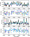 |
Fig. 10. RV temporal series for two subsets (upper and lower panels), covering most of the 3 year data from Dumusque et al. (2021): observations, model Mod2024 from Meunier et al. (2024), and three of the reconstructions corresponding to the assumption made on RVconvsp. |
We therefore conclude that taking into account more realistic ΔV laws does not bring a significant improvement, and that the observed small departure may be due to small effects outside active regions and network, for example flows at a larger scale around active regions. The very small difference between Mod2024 and the present reconstructions also shows that the simple laws used in Meunier et al. (2024) and in previous simulations Meunier et al. (2019a) is sufficient to derive RV synthetic time series with complex activity patterns such as in the solar case.
6. Conclusions
We analysed the difference ΔV in RV between magnetic structures and the quiet-Sun value as a function of the position on the disc. This was done on a single spectral line (Fe 6173 Å) in order to access a large quantity of homogeneous images. Although other spectral lines may have a different convective blueshift amplitude, this line has a moderate line depth. Although we confirm the dominant role of the magnetic flux in ΔV, the behaviour is not linear. In addition, the correlation between ΔV and the size of the structures observed in the literature may be dominated by the shape of the magnetic flux–size relation, but the magnetic flux is not the only factor. Unexpectedly, for a given magnetic flux, very small structures exhibit a larger ΔV compared to large magnetic structures; this is likely due to the fact that the estimation of ΔV is also impacted by the preferential location of flux tubes in strong downflows for small network structures, which is then mixed with the convective blueshift attenuation effect. For a given size, our results also suggest a stronger attenuation of the convective blueshift in more compact structures.
We confirm the variation in ΔV with μ obtained by Cegla et al. (2018) and Palumbo et al. (2024b), with a similar behaviour at first order for all structures and regions, apart from the amplitude. There may be a small trend for the position in μ of the sign reversal with magnetic flux, although this remains to be confirmed and explained. Comparison with MHD simulations including flux tubes with different properties should help interpret the results.
Finally, we find that what is usually called the quiet network, outside active regions, contributes to the rotational modulation and significantly to long-term RV variability. The RV reconstructed from observed ΔV does not agree significantly better with the observations than the model based on a simple law (Meunier et al. 2019a, 2024). The small departure between model and observation is not explained by the properties of active regions. Although complex structures are necessary to produce realistic synthetic time series and be representative activity pattern such as observed for the Sun, simple laws are sufficient to describe the convective blueshift contribution.
Acknowledgments
We thank the anonymous referee for their comments that helped improve the manuscript. This work was supported by the “Action Thématique de Physique Stellaire” (ATPS) of CNRS/INSU PN ASTRO co-funded by CEA and CNES. This work was supported by the Programme National de Planétologie (PNP) of CNRS/INSU, co-funded by CNES. HMI data, provided courtesy of NASA/SDO were retrieved from the JSOC archive. We thank Pierre Larue, Lionel Bigot, Suzanne Aigrain, and Nathan Hara for useful comments on this work.
References
- Al Moulla, K., Dumusque, X., Figueira, P., et al. 2023, A&A, 669, A39 [NASA ADS] [CrossRef] [EDP Sciences] [Google Scholar]
- Balthasar, H. 1985, Sol. Phys., 99, 31 [NASA ADS] [CrossRef] [Google Scholar]
- Beckers, J. M., & Nelson, G. D. 1978, Sol. Phys., 58, 243 [NASA ADS] [CrossRef] [Google Scholar]
- Beeck, B., Schüssler, M., Cameron, R. H., & Reiners, A. 2015, A&A, 581, A42 [NASA ADS] [CrossRef] [EDP Sciences] [Google Scholar]
- Berdyugina, S. V. 2005, Liv. Rev. Sol. Phys., 2, 8 [Google Scholar]
- Berger, T. E., Löfdahl, M. G., Shine, R. S., & Title, A. M. 1998, ApJ, 495, 973 [NASA ADS] [CrossRef] [Google Scholar]
- Borgniet, S., Meunier, N., & Lagrange, A.-M. 2015, A&A, 581, A133 [NASA ADS] [CrossRef] [EDP Sciences] [Google Scholar]
- Brandt, P. N., & Solanki, S. K. 1990, A&A, 231, 221 [NASA ADS] [Google Scholar]
- Buehler, D., Lagg, A., van Noort, M., & Solanki, S. K. 2019, A&A, 630, A86 [NASA ADS] [CrossRef] [EDP Sciences] [Google Scholar]
- Carlsson, M., Stein, R. F., Nordlund, Å., & Scharmer, G. B. 2004, ApJ, 610, L137 [NASA ADS] [CrossRef] [Google Scholar]
- Cavallini, F., Ceppatelli, G., & Righini, A. 1985, A&A, 143, 116 [NASA ADS] [Google Scholar]
- Cegla, H. M., Watson, C. A., Shelyag, S., et al. 2018, ApJ, 866, 55 [NASA ADS] [CrossRef] [Google Scholar]
- Cegla, H. M., Watson, C. A., Shelyag, S., Mathioudakis, M., & Moutari, S. 2019, ApJ, 879, 55 [NASA ADS] [CrossRef] [Google Scholar]
- Couvidat, S., Rajaguru, S. P., Wachter, R., et al. 2012, Sol. Phys., 278, 217 [NASA ADS] [CrossRef] [Google Scholar]
- Couvidat, S., Schou, J., Hoeksema, J. T., et al. 2016, Sol. Phys., 291, 1887 [Google Scholar]
- Criscuoli, S. 2013, ApJ, 778, 27 [Google Scholar]
- Criscuoli, S., Norton, A., & Whitney, T. 2017, ApJ, 847, 93 [Google Scholar]
- de la Cruz Rodríguez, J., Kiselman, D., & Carlsson, M. 2011, A&A, 528, A113 [Google Scholar]
- Desort, M., Lagrange, A.-M., Galland, F., Udry, S., & Mayor, M. 2007, A&A, 473, 983 [CrossRef] [EDP Sciences] [Google Scholar]
- Dravins, D. 1982, ARA&A, 20, 61 [NASA ADS] [CrossRef] [Google Scholar]
- Dravins, D. 2008, A&A, 492, 199 [NASA ADS] [CrossRef] [EDP Sciences] [Google Scholar]
- Dumusque, X. 2016, A&A, 593, A5 [NASA ADS] [CrossRef] [EDP Sciences] [Google Scholar]
- Dumusque, X., Boisse, I., & Santos, N. C. 2014, ApJ, 796, 132 [NASA ADS] [CrossRef] [Google Scholar]
- Dumusque, X., Borsa, F., Damasso, M., et al. 2017, A&A, 598, A133 [NASA ADS] [CrossRef] [EDP Sciences] [Google Scholar]
- Dumusque, X., Cretignier, M., Sosnowska, D., et al. 2021, A&A, 648, A103 [NASA ADS] [CrossRef] [EDP Sciences] [Google Scholar]
- Dunn, R. B., & Zirker, J. B. 1973, Sol. Phys., 33, 281 [NASA ADS] [Google Scholar]
- Ellwarth, M., Ehmann, B., Schäfer, S., & Reiners, A. 2023, A&A, 680, A62 [NASA ADS] [CrossRef] [EDP Sciences] [Google Scholar]
- Ermolli, I., Berrilli, F., & Florio, A. 2003, A&A, 412, 857 [NASA ADS] [CrossRef] [EDP Sciences] [Google Scholar]
- Foukal, P., Harvey, K., & Hill, F. 1991, ApJ, 383, L89 [NASA ADS] [CrossRef] [Google Scholar]
- Hagenaar, H. J., Schrijver, C. J., & Title, A. M. 2003, ApJ, 584, 1107 [NASA ADS] [CrossRef] [Google Scholar]
- Hara, N. C., & Delisle, J.-B. 2025, A&A, 696, A141 [NASA ADS] [CrossRef] [EDP Sciences] [Google Scholar]
- Harvey, J. W. 1984, in Probing the depths of a Star: the study of Solar oscillation from space, eds. R. W. Noyes, & E. J. Rhodes Jr., JPL, 400, 327 [Google Scholar]
- Harvey, K. L., & White, O. R. 1999, ApJ, 515, 812 [CrossRef] [Google Scholar]
- Haywood, R. D., Milbourne, T. W., Saar, S. H., et al. 2022, ApJ, 935, 6 [NASA ADS] [CrossRef] [Google Scholar]
- Herrero, E., Ribas, I., Jordi, C., et al. 2016, A&A, 586, A131 [NASA ADS] [CrossRef] [EDP Sciences] [Google Scholar]
- Immerschitt, S., & Schroeter, E. H. 1989, A&A, 208, 307 [Google Scholar]
- Ishikawa, R., Tsuneta, S., Kitakoshi, Y., et al. 2007, A&A, 472, 911 [NASA ADS] [CrossRef] [EDP Sciences] [Google Scholar]
- Kobel, P., Solanki, S. K., & Borrero, J. M. 2011, A&A, 531, A112 [NASA ADS] [CrossRef] [EDP Sciences] [Google Scholar]
- Kobel, P., Solanki, S. K., & Borrero, J. M. 2012, A&A, 542, A96 [NASA ADS] [CrossRef] [EDP Sciences] [Google Scholar]
- Kostik, R., & Khomenko, E. V. 2012, A&A, 545, A22 [NASA ADS] [CrossRef] [EDP Sciences] [Google Scholar]
- Lakeland, B. S., Naylor, T., Haywood, R. D., et al. 2024, MNRAS, 527, 7681 [Google Scholar]
- Livingston, W. C. 1982, Nature, 297, 208 [NASA ADS] [CrossRef] [Google Scholar]
- Löhner-Böttcher, J., Schmidt, W., Stief, F., Steinmetz, T., & Holzwarth, R. 2018, A&A, 611, A4 [Google Scholar]
- Macris, C. J. 1979, A&A, 78, 186 [Google Scholar]
- Makarov, V. V. 2010, ApJ, 715, 500 [NASA ADS] [CrossRef] [Google Scholar]
- Meunier, N. 2003, A&A, 405, 1107 [NASA ADS] [CrossRef] [EDP Sciences] [Google Scholar]
- Meunier, N., & Lagrange, A. M. 2019, A&A, 625, L6 [NASA ADS] [CrossRef] [EDP Sciences] [Google Scholar]
- Meunier, N., & Lagrange, A. M. 2020a, A&A, 638, A54 [NASA ADS] [CrossRef] [EDP Sciences] [Google Scholar]
- Meunier, N., & Lagrange, A. M. 2020b, A&A, 642, A157 [NASA ADS] [CrossRef] [EDP Sciences] [Google Scholar]
- Meunier, N., Desort, M., & Lagrange, A.-M. 2010a, A&A, 512, A39 [NASA ADS] [CrossRef] [EDP Sciences] [Google Scholar]
- Meunier, N., Lagrange, A.-M., & Desort, M. 2010b, A&A, 519, A66 [NASA ADS] [CrossRef] [EDP Sciences] [Google Scholar]
- Meunier, N., Lagrange, A.-M., Borgniet, S., & Rieutord, M. 2015, A&A, 583, A118 [NASA ADS] [CrossRef] [EDP Sciences] [Google Scholar]
- Meunier, N., Lagrange, A. M., Boulet, T., & Borgniet, S. 2019a, A&A, 627, A56 [NASA ADS] [CrossRef] [EDP Sciences] [Google Scholar]
- Meunier, N., Lagrange, A.-M., & Cuzacq, S. 2019b, A&A, 632, A81 [NASA ADS] [CrossRef] [EDP Sciences] [Google Scholar]
- Meunier, N., Lagrange, A. M., & Borgniet, S. 2020, A&A, 644, A77 [NASA ADS] [CrossRef] [EDP Sciences] [Google Scholar]
- Meunier, N., Pous, R., Sulis, S., Mary, D., & Lagrange, A. M. 2023, A&A, 676, A82 [NASA ADS] [CrossRef] [EDP Sciences] [Google Scholar]
- Meunier, N., Lagrange, A. M., Dumusque, X., & Sulis, S. 2024, A&A, 687, A303 [NASA ADS] [CrossRef] [EDP Sciences] [Google Scholar]
- Milbourne, T. W., Haywood, R. D., Phillips, D. F., et al. 2019, ApJ, 874, 107 [Google Scholar]
- Miller, P., Foukal, P., & Keil, S. 1984, Sol. Phys., 92, 33 [Google Scholar]
- Morinaga, S., Sakurai, T., Ichimoto, K., et al. 2008, A&A, 481, L29 [NASA ADS] [CrossRef] [EDP Sciences] [Google Scholar]
- Narayan, G., & Scharmer, G. B. 2010, A&A, 524, A3 [NASA ADS] [CrossRef] [EDP Sciences] [Google Scholar]
- Norris, C. M., Beeck, B., Unruh, Y. C., et al. 2017, A&A, 605, A45 [NASA ADS] [CrossRef] [EDP Sciences] [Google Scholar]
- Palumbo, M. L., Ford, E. B., Gonzalez, E. B., et al. 2024a, AJ, 168, 46 [NASA ADS] [CrossRef] [Google Scholar]
- Palumbo, M. L., Saar, S. H., & Haywood, R. D. 2024b, ApJ, 973, 11 [Google Scholar]
- Parnell, C. E., DeForest, C. E., Hagenaar, H. J., et al. 2009, ApJ, 698, 75 [Google Scholar]
- Romano, P., Berrilli, F., Criscuoli, S., et al. 2012, Sol. Phys., 280, 407 [CrossRef] [Google Scholar]
- Saar, S. H., & Donahue, R. A. 1997, ApJ, 485, 319 [Google Scholar]
- Scherrer, P. H., Schou, J., Bush, R. I., et al. 2012, Sol. Phys., 275, 207 [Google Scholar]
- Schmidt, W., Grossmann-Doerth, U., & Schroeter, E. H. 1988, A&A, 197, 306 [NASA ADS] [Google Scholar]
- Schou, J., Scherrer, P. H., Bush, R. I., et al. 2012, Sol. Phys., 275, 229 [Google Scholar]
- Solanki, S. K., Inhester, B., & Schüssler, M. 2006, Rep. Prog. Phys., 69, 563 [Google Scholar]
- Stief, F., Löhner-Böttcher, J., Schmidt, W., Steinmetz, T., & Holzwarth, R. 2019, A&A, 622, A34 [NASA ADS] [CrossRef] [EDP Sciences] [Google Scholar]
- Sulis, S., Mary, D., & Bigot, L. 2020, A&A, 635, A146 [NASA ADS] [CrossRef] [EDP Sciences] [Google Scholar]
- Thornton, L. M., & Parnell, C. E. 2011, Sol. Phys., 269, 13 [Google Scholar]
- Title, A., Tarbell, T., Topka, K., et al. 1988, Astrophys. Lett. Commun., 27, 141 [NASA ADS] [Google Scholar]
- Title, A. M., Tarbell, T. D., Topka, K. P., et al. 1989, ApJ, 336, 475 [NASA ADS] [CrossRef] [Google Scholar]
- Title, A. M., Topka, K. P., Tarbell, T. D., et al. 1992, ApJ, 393, 782 [NASA ADS] [CrossRef] [Google Scholar]
- van Driel-Gesztelyi, L., & Green, L. M. 2015, Liv. Rev. Sol. Phys., 12, 1 [Google Scholar]
- Vögler, A. 2005, Mem. Soc. Astron. It., 76, 842 [NASA ADS] [Google Scholar]
- Walton, S. R., Preminger, D. G., & Chapman, G. A. 2003, ApJ, 590, 1088 [NASA ADS] [CrossRef] [Google Scholar]
- Yeo, K. L., Solanki, S. K., & Krivova, N. A. 2013, A&A, 550, A95 [NASA ADS] [CrossRef] [EDP Sciences] [Google Scholar]
The perimeter is computed as the sum of the lengths of all pixel sides that are on the edge of the structure.
Appendix A: Comparison of Sets 1 and 2
Figure A.1 illustrates the difference in small-scale velocities and magnetic field between Sets 1 and 2 (i.e. before and after deconvolution). The slopes of the orange fit are 1.8 and 1.4 respectively. Criscuoli et al. (2017) found an increase in the granular contrast of a factor ∼2, which is consistent with the stronger velocities here. It is very similar to the Set 2 curve. Figure A.2 illustrates the differences in terms of size distribution between Set 1 and Set 2. Figure A.3 is similar to Fig. 5 but for Set 1.
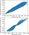 |
Fig. A.1. Comparison of the velocity fields (after the correction described in Sect. 3.2 including rotation, upper panel) and magnetic fields (lower panel) for part of an image at disc centre before and after deconvolution. Each point corresponds to one pixel. |
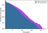 |
Fig. A.2. Distribution of the structure sizes before and after deconvolution. |
Appendix B: Quiet-Sun reference
Figure B.1 shows the average velocity of the quiet Sun as a function of μ. We used boxes with a size of 8x8 pixels with a low average magnetic field to evaluate this quiet-Sun average velocity (see Sect. 3.2), which is then used to correct all other velocities.
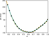 |
Fig. B.1. Velocity vs μ for quiet boxes only (see text) for Set 1. The orange curve corresponds to interpolated values and the green curve to a polynomial fit of degree 4. |
Appendix C: Times series
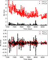 |
Fig. C.1. Time series before scaling representing RVconvpl and RVconvsp (upper panel), and RVphotpl (middle panel) and RVphotsp (lower panel). |
All Tables
All Figures
|
Fig. 1. Example of maps (only one-quarter of the field is shown). Shown are the intensity map and the corrected Dopplergram (upper row) and the magnetic flux map and segmented map (lower row), for Set 2. |
| In the text | |
|
Fig. 2. Zoomed-in image at disc centre on a segmented map, illustrating the magnetic structures in different size ranges, for Set 1 (left panel) and Set 2 (right panel). The two maps are separated by 2.5 hours, which distorts the structures only slightly. |
| In the text | |
|
Fig. 3. ΔV as a function of average magnetic flux for the pixel approach (upper panel) and the box approach (lower panel) at disc centre (μ > 0.95), for Set 1 (dashed) and Set 2 (solid). The black curve corresponds to points, and the colours to the different structure sizes (of the structure the pixel or the box it belongs to). We note the difference in scales in the two panels. |
| In the text | |
|
Fig. 4. ΔV as a function of average magnetic flux for the structure approach at disc centre (μ > 0.95) vs size for different ranges of B (upper panel) and vs B for different ranges of size (lower panel), for Set 1 (dashed) and Set 2 (solid). The black curves are for all B (all sizes). The vertical black lines correspond to the typical granular size (dashed), the box size (solid), and the 20 ppm scale (network-active region interface, dotted). |
| In the text | |
|
Fig. 5. Upper panel: B vs structure size for Set 2. The coloured area show the 1σ dispersion, and the orange dots a polynomial fit on the binned B vs size. Middle panel: ΔV vs size for the two categories of structures, with B larger than the orange curve in green, and with B smaller than the orange curve in magenta. Lower panel: Distribution of the perimeter/size ratio for these two categories of structures. The vertical black lines correspond to the typical granular size (dashed), the box size (solid), and the 20 ppm scale (network-active region interface, dotted). |
| In the text | |
|
Fig. 6. ΔV vs μ for the pixel (upper panel), structure (middle panel), and box (lower panel) approaches, for different categories of B. |
| In the text | |
|
Fig. 7. Values of μ for which ΔV changes sign vs B for the three approaches, pixel (violet), structure (cyan), and box (pink), for Set 2. |
| In the text | |
|
Fig. 8. ΔV vs μ for different ranges in B (structure approach), for Set 2, and different ranges in size: < 2 ppm (pink), 2–20 ppm (violet), and > 20 ppm (cyan). |
| In the text | |
|
Fig. 9. Smoothed time series for the five categories in size (upper panel) and zoomed in on the residuals (lower panel). |
| In the text | |
|
Fig. 10. RV temporal series for two subsets (upper and lower panels), covering most of the 3 year data from Dumusque et al. (2021): observations, model Mod2024 from Meunier et al. (2024), and three of the reconstructions corresponding to the assumption made on RVconvsp. |
| In the text | |
|
Fig. A.1. Comparison of the velocity fields (after the correction described in Sect. 3.2 including rotation, upper panel) and magnetic fields (lower panel) for part of an image at disc centre before and after deconvolution. Each point corresponds to one pixel. |
| In the text | |
|
Fig. A.2. Distribution of the structure sizes before and after deconvolution. |
| In the text | |
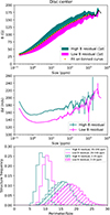 |
Fig. A.3. Same as Fig. 5, but for Set 1. |
| In the text | |
|
Fig. B.1. Velocity vs μ for quiet boxes only (see text) for Set 1. The orange curve corresponds to interpolated values and the green curve to a polynomial fit of degree 4. |
| In the text | |
|
Fig. C.1. Time series before scaling representing RVconvpl and RVconvsp (upper panel), and RVphotpl (middle panel) and RVphotsp (lower panel). |
| In the text | |
Current usage metrics show cumulative count of Article Views (full-text article views including HTML views, PDF and ePub downloads, according to the available data) and Abstracts Views on Vision4Press platform.
Data correspond to usage on the plateform after 2015. The current usage metrics is available 48-96 hours after online publication and is updated daily on week days.
Initial download of the metrics may take a while.