| Issue |
A&A
Volume 707, March 2026
|
|
|---|---|---|
| Article Number | A125 | |
| Number of page(s) | 13 | |
| Section | Numerical methods and codes | |
| DOI | https://doi.org/10.1051/0004-6361/202555183 | |
| Published online | 10 March 2026 | |
Periodicities in radio emissions from Jupiter’s magnetosphere and consequences for radio emissions from star–exoplanet systems
1
LIRA’ Observatoire de Paris, Université PSL, Sorbonne Université, Université Paris Cité, CY Cergy Paris Université, CNRS,
92190
Meudon,
France
2
ORN, Observatoire Radioastronomique de Nançay, Observatoire de Paris, CNRS, Univ. PSL, Univ. Orléans,
18330
Nançay,
France
3
Aix Marseille Université, CNRS, CNES, LAM,
Marseille,
France
4
LPC2E – Université d’Orléans/CNRS,
France
5
LATMOS, CNRS – Sorbonne Université – CNES,
Paris,
France
6
Université Paris Cité and Université Paris Saclay, CEA, CNRS, AIM,
91190
Gif-sur-Yvette,
France
★ Corresponding author: This email address is being protected from spambots. You need JavaScript enabled to view it.
Received:
16
April
2025
Accepted:
23
January
2026
Abstract
Context. The search for radio signals from exoplanets or star-planet interactions is a topic of major scientific interest, as it is likely the best way to detect and measure a planetary magnetic field and, therefore, to probe the inner structure of exoplanets. However, detecting these radio emissions is challenging, since they are anisotropic by nature, sporadic, and of low intensity because of their great distances, and because the sky cannot be monitored continuously.
Aims. The aim of this article is to demonstrate the relevance of using statistical tools to detect periodic radio signals in unevenly spaced observations and to identify the implications of the measured period.
Methods. The identification of periodic radio signals was achieved here through a Lomb-Scargle analysis. The technique was first applied to simulated astrophysical observations with controlled simulated noise. This allowed us to characterise the origin of spurious detection peaks in the resulting periodograms - as well as to identify peaks corresponding to real periods in the studied system - and to combination or beat periods.
Results. The method was validated using a real signal, with ∼1400 hours of data from observations of Jupiter’s radio emissions by the NenuFAR radio telescope over more than six years, in order to detect the periodicities of Jovian radio emissions (auroral and induced by the Galilean moons).
Conclusions. We demonstrate with the simulation that the Lomb-Scargle periodogram allows us to correctly identify periodic radio signals, even in a diluted signal. On real measurements, it correctly detects the rotation period of the strong signal produced by Jupiter and the beat period of the emission triggered by the interaction between Jupiter and its Galilean moon Io, but also possibly weaker signals, such as those produced by the interaction between Jupiter and Europa or between Jupiter and Ganymede. It is important to note that secondary peaks in the Lomb-Scargle periodogram appear at the beat and combination periods among all the detected signal periodicities (i.e. real signals, but also periodicities due to regular observation intervals). These secondary peaks can then be used to strengthen the detection of weak signals. Finally, the importance of the number of observation windows used in the Lomb-Scargle analysis is discussed, as well as the data’s time and frequency resolutions in increasing its efficiency.
Key words: magnetic fields / plasmas / waves / methods: data analysis / methods: statistical / planet-star interactions
© The Authors 2026
 Open Access article, published by EDP Sciences, under the terms of the Creative Commons Attribution License (https://creativecommons.org/licenses/by/4.0), which permits unrestricted use, distribution, and reproduction in any medium, provided the original work is properly cited.
This article is published in open access under the Subscribe to Open model. This email address is being protected from spambots. You need JavaScript enabled to view it. to support open access publication.
1 Introduction
The most successful way to image stellar magnetic fields is to use spectro-imaging techniques such as Zeeman Doppler imaging (ZDI), which can detect a stellar magnetic field down to 0.8 G (Brown et al. 2022). However, in the case of exoplanetary magnetic fields, the spectrum of the exoplanet is usually combined with that of the star, making it difficult to extract the exoplanet’s polarimetric signature, and the photon noise can severely limit the possibility of detecting this potentially weak polarimetric signal. Finally, the exoplanet magnetic field might also not be strong enough to produce a sufficient Zeeman effect on the atoms or molecules of the exoplanet’s atmosphere, the composition and temperature of which differ from those of a star (for a low limit for low temperatures, see, e.g. Kuzmychov et al. 2017, which presents the detection of a magnetic field of 5 kG for the brown dwarf LSR J1835+3259 of spectral type M8.5V). Consequently, ZDI is unable to characterise exoplanetary magnetic fields.
Indirect detections of exoplanetary magnetic fields have been achieved using techniques based on planet-modulated chromospheric emission (Cauley et al. 2019) or neutral atomic hydrogen absorption during transit (Ben-Jaffel et al. 2022). Another way to study and characterise exoplanetary magnetic fields is through the observation of exoplanetary auroral radio emissions. These emissions are produced by the cyclotron maser instability (CMI, Treumann 2006) at all magnetised planets in our Solar System (Zarka 1998) and are particularly well known and studied in situ on Earth, Jupiter, and Saturn (Wu & Lee 1979; Le Queau et al. 1984b,a; Wu 1985; Pritchett 1986a; Lamy et al. 2010; Mutel et al. 2010; Kurth et al. 2011; Louarn et al. 2017, 2018; Louis et al. 2023a; Collet et al. 2023, 2024). They occur at or near the fundamental frequency of the local electron cyclotron frequency:
 (1)
(1)
with e and me being the charge and mass of an electron and B the local magnetic-field amplitude. As the magnetic-field amplitude decreases with increasing altitude above the atmosphere, auroral radio emissions span a broad range of frequencies along the magnetic-field lines, provided the ratio between the plasma frequency and the cyclotron frequency is less than ∼0.1 (from theoretical work on the CMI and from in situ measurements by Juno at Jupiter; Zarka et al. 2001; Chen et al. 2002; Lee et al. 2013; Louis et al. 2023a; Collet et al. 2024, 2025). The minimal frequency for the emission is therefore reached at high altitudes (several body radii), while the maximal frequency corresponds to the maximal cyclotron frequency near the planetary surface.
Consequently, detecting these radio emissions provides information about the local magnetic field. For example, in our Solar System, Jovian auroral radio emissions were first detected (above the ionospheric cut-off at 10 MHz) in 1955 by Burke & Franklin (1955), making Jupiter’s magnetosphere the first to be identified using the radio radiation. Jovian auroral radio emissions extend from a few kilohertz (kilometric range) up to 40 megahertz (decametric range), corresponding to a magnetic field with a maximal amplitude of about 15 G (Connerney et al. 2022).
These radio emissions are highly anisotropic. They are produced along the edges of a hollow cone, ∼1–2° thick, with an opening angle relative to the local magnetic-field vector, B, varying from ∼70° to 90° depending on the type of electron distribution function and the emission frequency (Pritchett 1986b; Treumann 2006; Hess et al. 2008). Consequently, the visibility of these emissions strongly depends on the observer’s position in the reference frame of the emitting body (Lamy et al. 2023b). For instance, in the case of emissions induced by the moon Io (Bigg 1964), a terrestrial observer located approximately in the plane of the Jovian equator can only see the emissions when Io is in quadrature (Marques et al. 2017a). Saturn-like auroral radio emissions (fast rotator, sensitive to stellar wind) are mostly visible for an observer in the morning sector, and hence also in quadrature (Lamy 2017; Lamy et al. 2023b, 2008; Kimura et al. 2013; Nakamura et al. 2019). For Earth-like auroral radio emissions (highly sensitive to stellar wind) the maximal chance of detection is for an observer located in the nightside sector (Waters et al. 2022; Lamy et al. 2023b; Louis et al. 2023b). Finally, Jupiter-like auroral (non-satellite-induced) radio emissions (strongly magnetised and fast rotator planet, partially sensitive to stellar winds) do not require any preferred position of observation for most of their components (Zarka et al. 2021; Louis et al. 2021; Lamy et al. 2023b; Boudouma et al. 2023).
Another important characteristic of auroral radio emissions is their strong polarisation, which is almost 100%. These emissions are produced in the extraordinary mode (so-called R-X mode) and are therefore circularly or elliptically polarised in the right-handed (RH) sense relative to the magnetic field at the source. The observed polarisation thus depends on the magnetic hemisphere: it is RH when the (B, k) angle is acute (with k being the radio-wave vector) and left-handed (LH) when the (B,k) angle is obtuse. However, these signals are weak at stellar distances and highly sporadic. To detect these weak astrophysical signals (Zarka et al. 2018), it is crucial to use prediction tools (e.g. ExPRES, Louis et al. 2019; PALANTIR, Mauduit et al. (2023); phase prediction1, Zhang et al. 2025a). Another problem is that the detections published so far have been individual bursts (Callingham et al. 2021a,b, 2023, 2024; Tasse et al. 2025; Turner et al. 2021, 2023, 2024; Vedantham et al. 2020); thus, it is not possible to draw conclusions about their origin in the observed stellar systems (either from the star itself, an exoplanet, or a star-planet interaction).
With sufficient observation hours over an extended period using sensitive radio telescopes (Turner et al. 2019), it should in principle become possible to search for periodicity in the signal, instead of searching for individual weak and sporadic radio emissions. However, a significant challenge arises from the uneven spacing of these observations over time. Due to the limited observability of the sources (not 24 hours a day), observation biases (at 24 hours because of the radio frequency interferences that pollute the observations, and at 23.93 hours, which is the sidereal period), and high observing pressure on giant telescopes such as NenuFAR (Zarka et al. 2020), regular observations are impractical. Consequently, periodicity search techniques capable of handling unevenly spaced observations are required, and the Lomb-Scargle (LS) periodogram such as the one provided by the Astropy Python package (Astropy Collaboration 2013, 2018, 2022; VanderPlas et al. 2012; VanderPlas & Ivezic 2015) is an excellent option for this purpose. The LS periodogram has, for instance, proven to be successful in tracking the double radio period of Saturn’s kilometric radiation (e.g. Lamy 2017), the period of Jovian quasi-periodic bursts (Kimura et al. 2011), and the brown-dwarf period (e.g. Kao et al. 2018; Vedantham et al. 2023; Bloot et al. 2024).
In this work, a practical test was conducted on real Nen-uFAR data. To understand how the LS periodogram performs on NenuFAR data, a first test was done on a simulated signal (see Section 2). Initially, a sine wave with a known periodicity and random observation gaps is used. Next, a similar simulation was produced, but this time the observation windows and gaps between observations were controlled to study the impact of observation regularity on the LS periodogram, hence mimicking real observing conditions. Finally, the signal was embedded in random noise with a normal distribution, and we studied how varying the signal-to-noise ratio affects the detection of the underlying periodic signal. In Section 3, the LS periodogram is applied to real observations of Jupiter’s radio emissions acquired over a six-year interval with the NenuFAR radio telescope to analyse the periodicities detected. Finally, this study is summarised and discussed in Section 4 to highlight the constraints and limitations of using this technique to detect radio emissions by searching for signal periodicity.
2 Simulations
In the first simulation (see Figure 1, left), a sinusoidal signal wave was created (in blue) with a periodicity of Tsine = 12.90 hours (with an amplitude between −1 and 1; in preparation for the analysis given in Section 3 of the data in circular polarisation, which therefore has a ratio of Stokes parameters V over I between −1 and 1) over five years (only a few tens of days are shown for the sake of readability) with a time resolution of 600 seconds. A random selection of 2.65% of the data points in the time series is then made for analysis. By anticipating the real signal, a periodicity of 12.9 hours was chosen, as it is close to the real physical periodicity investigated in Section 3. The percentage of kept signal was chosen on the basis of the percentage of data actually observed, which we analyse in Section 3. The corresponding LS periodogram is shown on the right of Figure 1. The highest peak (by far) in the periodogram is located at 12.9 hours. The 95% confidence level, based on a randomisation test, is also shown. Our randomisation test consists of taking the time series under consideration, shuffling the values randomly over time and calculating the resulting LS periodogram. For this test to have sufficient statistical validity, it was repeated 1000 times. The confidence levels therefore indicate the percentage of times the highest peak reaches this power value. This is equivalent to the false-alarm probability (FAP) using the bootstrap method in the LS Astropy Python package. In the case of this first simulation, the 95% confidence level is obviously very low, as there is only signal given as input; moreover, the portion of kept signal is completely random.
In Figure 2, we show the simulation of the same sinusoidal wave (i.e. with a Tsine = 12.9 h periodicity and a time resolution of 600 seconds), but this time more realistic values were used to select the kept signals. 2.65% of the kept signal was gathered into 125 intervals of eight hours separated by N × 23.93 hours (with N = 1,2,3,4,...), i.e. the sidereal day. These values were chosen on the basis of the real observational values of the target studied in Section 3. The corresponding LS periodogram is shown on the right of Figure 2. The highest peak is still located at 12.9 hours, but this time several other peaks are also visible, mainly at 27.99, 8.38, and 6.21 hours.
In Figure 3, the effect of the windowing on the LS periodogram is studied. In this figure, the same observation intervals as in Figure 2 are taken, but all values are equal to one (left panel). In the LS periodogram (right panel), the input sinusoidal periodicity is not visible anymore. However, two major peaks are detected at 23.93 and 11.97 hours.
To identify the origin of these different peaks, the possible combinations between different periodicities need to be studied. The two major combinations are (i) the difference between the two periodicities (in frequency), i.e. the beat period:
 (2)
(2)
which corresponds in time periodicity to
 (3)
(3)
and (ii) the sum of the two periodicities (in frequency), i.e. the combination period:
 (4)
(4)
which corresponds in time periodicity to
 (5)
(5)
with m = 1,2,....
In our case, the simulation introduces three possible periodicities: Tsine = 12.9 h; the interval between two observations, Tgap = 23.93 h; and the length of the observations, Tobs = 8 h. Tobs cannot really be considered as a periodicity since it is the duration of each observation, though it does have an effect on the windowing. Several combinations are thus possible, which are summarised in Table 1. Therefore, the peaks observed in Figure 2 can be explained by (i) the beat period between Tsine and Tgap, and (ii) the combination period between Tsine and Tgap, for m = 1 and m = 2.
The two major peaks seen in Figure 3 are explained by Tgap itself, i.e. at Tgap and  . The two smaller peaks are explained by the combination period between Tobs and Tgap, for m = 1 and m = 2. All these peaks are therefore only due to the windowing of the observations (the periodicity of the observation length and interval between two consecutive observations). The 95% confidence level is obviously at the value of the highest peak, since all data points are equal to one, and shuffling them randomly over the time intervals makes no difference to the LS analysis.
The third simulation (see Figure 4 left) is the same as the one in Figure 2, to which a normal distribution was added to dilute the sinusoidal wave in order to move a little closer to a real signal and away from the idealised case of the previous figure and to obtain an LS periodogram that is close to what we show in Section 3. The sinusoidal wave is still centred on zero, with an amplitude between −1 and +1, and a rms of σsine = 0.71. The normal distribution generated has a standard deviation of σnormal distribution = K × σsine, with K being the dilution factor (i.e. the signal-to-noise ratio). This distribution is then added to the sinusoidal wave, and the standard deviation of this combined signal, σcombined, is calculated. To obtain a combined signal with the same properties as the original signal, in order to decrease its signal-to-noise ratio (S/N), the combined signal is normalised by dividing by the dilution factor K. This new signal is called the ‘corrected combined signal’. Finally, as for the previous simulations, 2.65% of the signal is kept and gathered in 125 intervals of eight hours separated by N × 23.93 hours (with N = 1,2,3,4,...) and a time resolution of 600 seconds.
Figure 4 shows the results with a dilution factor of K = 15 (light grey). As one can see (left panel), the standard deviation of the original sinusoidal wave (light blue) and of the corrected combined (red) signal is the same. However, the LS periodogram (right panel) is different from that in Figure 2: as soon as noise is added, a forest of peaks appears. The period of the input sine, Tsine = 12.90 h, is still detected, even though the noise in the LS periodogram has drastically increased, and the value of the peaks has drastically decreased. The other two highest peaks are still located at 8.38 hours (combination period between Tgap and Tsine) and at 27.99 hours (beat period between Tgap and Tsine). This latter LS periodogram strongly resembles what is observed for real data, as presented in the following section. The 95% confidence level is located at higher LS power values, confirming that the noise is much more present in that case; however, the three highest peaks, related to Tsine are still well above the 95% level. In this case, the noise is entirely random. Although many periods are visible in the LS periodogram (the forest of peaks), all of them remain below the 95% confidence level. As we show later, this will not be the case with real noise.
Finally, the evolution of the LS periodogram as a function of the number of samples included is presented in Appendix A, Figure A.1. For the simulated signal, the S/N of the LS periodogram -denoted S/N(LS) and calculated as the LS power divided by the standard deviation of the LS periodograms- is evolving as the square root of the number of samples included in the LS analysis (see bottom panel). The top panel shows that for this simulated signal (diluted into noise by a factor K = 8) it takes N ≃ 20 samples for the maximal peak in the LS periodogram to be stabilised along the value of Tsine.
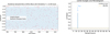 |
Fig. 1 (Left) Randomly spaced sinusoidal wave with period Tsine = 12.90 h. Only a few days of the entire five-year interval are shown in order to show the sinusoidal signal clearly. (Right) Corresponding LS periodogram. The 95% confidence level (based on a randomisation test) is indicated for the LS periodogram. It is very low in this case as only signal is given (no noise). |
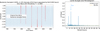 |
Fig. 2 (Left) Semi-regularly spaced sinusoidal wave with period Tsine = 12.90 h. The samples are gathered into 125 intervals of eight hours, spaced by N × 23.93 hours (with N = 1,2,3,4,...). (Right) Corresponding LS periodogram. The 95% confidence level is also indicated. It is also very low in this case as only a signal is given (no noise). |
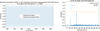 |
Fig. 3 Same as Figure 2, but with all values of the sinusoid at 1 in order to show the effect of the windowing on the LS periodogram. The 95% confidence level is also indicated. As all values are saturated to 1, randomly shuffling the values does not change the LS analysis, and the 95% confidence level is at the values of the highest peaks (due to the sidereal periodicity at N × 23.93 hours). |
Possible fundamental, beat, and combination periods that could be expected due to the sine, observed, and gap periods in our simulated signal.
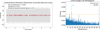 |
Fig. 4 (Left panel) Semi-regularly spaced sinusoidal wave with period Tsine = 12.90 h (light blue), normal distribution with a standard deviation of σ = K × σsin with K = 15 (light grey), and combined signal with higher signal-to-noise ratio (red points). The samples are gathered into 125 intervals of eight hours spaced by N × 23.93 hours. (Right panel) Corresponding LS periodogram. The 95% confidence level is also shown in the LS periodogram. |
3 Application to real signal: Jupiter observation with NenuFAR
In this section, we present an analysis of real observations of Jupiter’s radio emissions collected using the NenuFAR radio telescope2 (Zarka et al. 2020). The Jupiter observations consist of time-frequency arrays of the Stokes parameters, which were acquired with the NenuFAR beam-forming mode throughout a dedicated long-term key programme from September 2019 to November 2022 (early science phase) and then to 2025 (regular cycles 1 to 5). The number of available mini-arrays (MA; sub-groups of 19 antennas) increases over time (from 56 in 2019 to −80 after April 2022, minus the ones under maintenance). The observations used a typical 84 ms × 12 kHz sampling and were scheduled close to the perijoves of the Juno spacecraft orbiting Jupiter (Bolton et al. 2017). From cycles 2 to 4, the observations were additionally scheduled to search for decametric emissions induced by Io, Europa, and Ganymede (Lamy et al. 2023a). It is also worth mentioning that the effective area of Nen-uFAR antennas, and therefore the final instrumental sensitivity, regularly increased from 2019 to 2025. Overall, this large NenuFAR Jupiter dataset consists of 176 independent observations of ~8 hours, corresponding to a total exposure of ~1400 hours. The interval between the start times of two consecutive observations is N × 23.93, with N = 1,2,3,4,5,..., corresponding to N × 23 hours, 55 minutes, and 48 seconds -the duration for Jupiter to return to the meridian for a fixed observer on Earth. This periodicity is also very close to the sidereal day, i.e. 23 hours, 56 minutes, 4 seconds ≃ 23.934 hours. Therefore, these two periodicities will probably merge in the LS analysis, and it is hereafter referred to as TDay.
A typical observation is displayed in Figure 5. The top panel shows the Stokes I parameter with pre-processing applied. This preprocessing of the data consists of a time-frequency integration of the data to ~251 msec ×-24 kHz. During this integration, the PATROL algorithm (Vasylieva 2015; Zakharenko et al. 2013; Turner et al. 2017) is used to store bad pixels as a weight mask of the same size (nt,nf) as the reduced Stokes I data. Each value of the flag mask is the fraction (0...1) of the good pixels integrated to obtain the corresponding pixel in the reduced data. This weight array is thresholded at 50% (i.e. values of ≤0.5 are set to zero and values >0.5 are set to one). The bottom panel displays the degree of circular polarisation, defined as the ratio between Stokes V and Stokes I, with values ranging between −1 and 1.
In this figure, radio frequency interference (RFI) can clearly be seen in the Stokes I data below 20 MHz, before 23:00 UTC and after 04:00 UTC, i.e. during the daytime. As these RFIs are almost not circularly polarised, they are not visible in the V/I data. In both the Stokes I and V/I ratio, radio emissions are clearly visible between 23:00 and 05:00. These emissions display different degrees of circular polarisation, providing insight into the polarisation characteristics of the emissions and their hemisphere of origin: V/I> 0 corresponds to LH emissions therefore originating from the southern hemisphere of Jupiter, while V/I < 0 corresponds to RH emissions therefore originating from the northern hemisphere of Jupiter. Using the Jupiter Probability Tool (Cecconi et al. 2023), these features are identified as Io-induced emissions.
In the following, the focus is on this degree of circular polarisation, since RFI and sky background have little or no circular polarisation, thereby resulting in a better S/N. In addition, the fact that |V/I| ≤ 1 -while the values of |V| vary over several orders of magnitude- allows the LS method to work better.
Using the Louis et al. (2025a) pipeline, the observations were further processed to a time resolution of 600 seconds and a frequency resolution of 1 MHz, ranging from 8 to 88 MHz, to further increase the S/N (to access the processed data, please see Louis et al. 2025b). Note here that the data up to 88 MHz were kept, since they were acquired up to this frequency from April 2023, with a view to observing synchrotron radiation. However, the circular polarisation expected for this radiation is weak-to-non-detectable in this frequency range (Girard et al. 2016), as Jupiter’s radiation belt system is not resolved with NenuFAR resolution, which may lead to circular polarisation smearing. Therefore, only circular polarisation data up to 40 MHz are analysed, i.e. the upper limit of auroral radiation.
Table 2 lists the fundamental and periods at which one can expect to see signals for Jupiter, TJupiter (corresponding to auroral radio emissions), and its various moons that control part of the Jovian radio spectrum: Io, TIo; Europa, TEuropa; and Ganymede, TGanymede. In addition, the day/observation periodicity, TDay, was added. The different combinations of these periods are listed; i.e. the beat and combination periods that can be expected to be found in the LS periodograms that follow. The average length of the observations are not included in the calculation of the beat or combination periods; as seen in Section 3, this does not influence the periodograms (except in the case of the study of pure windowing).
Figure 6A shows the degree of circular polarisation (Stokes V/I) measurements within 5 MHz frequency bands. Figures 6B-G show periodograms of the S/N of the LS power - noted S/N(LS) - for 5 MHz frequency bands in the [8, 38[ MHz range. The level of the noise in each frequency band is approximated by the standard deviation of the LS periodogram. The 95% confidence level is shown in each panel. In the case of real data, this confidence level is still quite low, and well below a large number of peaks. As indicated at the end of the Section 2, for data with ‘structured windows’, this produces data aliasing and high noise correlation. As a result, the FAP tends to be underestimated by the bootstrap method (see, e.g. Section 7.4.2.3 in VanderPlas 2018). To partially eliminate noise and enable comparison between different frequency bands (where noise levels may vary), the LS periodogram is plotted as a function of the S/N, calculated as the LS power (in each frequency band) divided by the standard deviation of the LS periodograms (in each frequency band). It should be noted that this S/N should not be considered as a confidence sigma, but rather it serves to define a common threshold for all frequency bands. Figure 7 shows a summary in 2D (observed radio frequency versus LS periodicities) of Figs. 6B-G for 1 MHz bands. The data in this figure were thresholded by calculating the 99.99th percentile of the overall 2D distribution, resulting in a value of S/N(LS) = 15.
Depending on the frequency, different peaks are visible. First, peaks are detected at 9.93 hours within the range of ∼13-25 MHz and at 4.97 hours between 19 and 24 MHz, which corresponds to TJ, the fundamental of the Jupiter rotation period, and TJ/2, half a Jupiter rotation period. Two other peaks are linked to Io: one detected at 12.96 hours from ∼23 to 33 MHz, which corresponds to Tbeat IJ, the beat period between Jupiter and its Galilean moon Io (which corresponds to the synodic period of Io); and a second one at 21.23 hours from 26 to 33 MHz, corresponding to TIo/2, which is Io's half orbital period, implying that the LS analysis detects radio emissions related to Jupiter itself and induced by Io (at Io's revolution or Io-Jupiter beat, or in that case synodic periods). The higher S/N(LS) for TJupiter-Iobeat than for TIo highlights the fact that Jupiter's magnetic field is not axisymmetric. This is furthermore emphasised by the S/N(LS) values that are higher for TIo/2 than for TIo. Peaks related to Jupiter are seen at lower frequencies than those related to Io, which is due to the topology of the Jovian magnetic fields (Io-induced radio emissions reach higher frequencies, see, e.g., Marques et al. 2017a).
Below ∼25 MHz, another strong peak is detected at ∼23.93 hours. This corresponds to Tday, which is both the sidereal period for Jupiter to be visible in the sky and the sidereal day. The former periodicity only affects the Jovian auroral radio emissions (usually seen at <25 MHz, due to Jupiter magneticfield topology connected to the magnetic-field lines producing these emissions) as they can be observed almost every time Jupiter is visible in the sky, while Io-induced emissions are visible only if Io is in quadrature. The latter affects the background radio signal visibility – the RFI is most probably still visible in the V/I data – which is also only visible at ≤20 MHz (see Figure 5), since this periodicity is only detected at low frequencies. A harmonic of this peak is also visible at TD/2.
Four other peaks are also visible. Two above 23 MHz are related to Io's periods (Keplerian and beat with Jupiter): (i) at 28.27 hours from 23 to 33 MHz corresponding to Tbeat D.IJ, which is the beat period between the Tbeat IJ and TD periodicities; (ii) at 33.27 hours from 24 to 32 MHz, corresponding to Tbeat I/2-IJ, which is the beat period between TIo/2, i.e. the Io's half-orbital period, and the Tbeat IJ period. Two are contained in the 13-25 MHz range and are related to Jupiter's period: (i) Tcomb JD, which is the combination period between the Jupiter, TJ, and the day, TD, periodicities at 7.02 hours from 13 to 23 MHz and (ii) Tbeat DJ, which is the beat period between the Jupiter, TJ, and the day, TD, periodicities at 16.97 hours from 13 to 25 MHz.
Interestingly, the peaks at Tcomb DJ, Tbeat DJ, Tbeat D-IJ, and Tbeat I/2-IJ each combine individual LS power at two different frequencies, thereby strengthening the detection of periodic signals at Tbeat IJ, TI/2, and TJ, providing stronger evidence for these periodicities. Figure A.2 displays (bottom panel) the evolution of the S/N(LS) as a function of observation samples inserted into the LS periodogram for some of the major LS periodicity peaks. It shows that some of beat or combination periodicity peaks (e.g. Tcomb DJ and Tbeat DJ) can be almost as high as fundamental periodicities (e.g., Tbeat IJ or TIo). Figure A.1, top panel, shows that it takes N ≳ 4-15 samples (i.e. observations) to achieve stability in the values of the periodicities.
Other potential periodicities could be linked to two additional Galilean moons -Europa and Ganymede- as they also induce radio emissions in the decametric range. (Louis et al. 2017, 2023a; Zarka et al. 2018; Jácome et al. 2022). As for Io, the expected periodicity would have been at the beat period with Jupiter, i.e. Tbeat Europa-Jupiter = 11.24 hours and Tbeat Ganymede-Jupiter = 10.54 hours. No significant peaks are visible at these periodicities; only a small one is observed at Tbeat Europa-Jupiter (LS power = ~ 0.014) in Figures 6E.F. This is not a surprise, as almost all radio emissions detected in the NenuFAR Jupiter observation are known to be associated with the Io-Jupiter interaction or to Jupiter itself. The periodic signals at Tbeat Europa-Jupiter and Tbeat Ganymede-Jupiter are further discussed in the following paragraphs.
Based on the detected peaks at specific periodicities, the goal is to constrain the times at which the signals contributing to the LS power were observed. The LS periodogram, initially calculated over the data acquired during an interval in excess of six years, raises the question of whether similar analyses could be performed over shorter time spans. To address this, Figure 8 displays the S/N of the LS periodograms calculated over time for different frequency ranges using a sliding window approach. Each window spans 500 days and slides every two days. Note that the effect of the window size and slide was studied: after several tests, it was determined that a window size of 200-500 days and a slide of the window of ≲ 1% of the window size yields the best results. A window that is too small (e.g. 100 days) induces a large increase in the LS noise. This can also be understood by looking at Figure A.2: 200 days corresponds to approximately 20 samples.
Figure 8 is a zoomed-in view of the 4-20 hour LS periodicities highlighting most of the periodicities of interest, including Tbeat D-J, Tbeat I-J, Tday/2, Tbeat E-J (for Europa-Jupiter), Tbeat G-J (for Ganymede-Jupiter), TJupiter, Tcomb D-J, and TJupiter/2, presented from top to bottom in each panel. For the [8, 18] MHz range (Figure 8A), a notably large peak is centred at Tday/2 = 11.97 hours due to both the Earth rotation period and the time it takes for Jupiter to return to the meridian. Some peaks are closely aligned with Jupiter periodicities at TJupiter, TJupiter/2, or at Tbeat D-J and Tcomb D-J ; or with the Io-Jupiter beat period of Tbeat I-J (e.g. Figures 8D-F). Interestingly, an enhancement of the S/N of the LS power is visible at Tbeat E-J in the [13, 18[ MHz frequency range in 2021 (panel 8B) and in the [23, 28] frequency range in 2023-2024 from mid-cycle 2 to mid-cycle 3 (panel 8D) and at Tbeat G-J in the [13, 18[ MHz frequency range mainly during cycle 1 and also from time to time during the early science phase ≤ 2022 (panel 8B). These results emphasise the potential of LS periodograms, calculated over shorter time spans, to reveal temporal variations in signal periodicities and to identify specific intervals of enhanced observational significance.
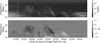 |
Fig. 5 Typical NenuFAR ‘time (UTC) versus frequency (in MHz) spectrogram, of Jupiter signal. (Top panel) Stokes I with data preprocessing applied (see text). (Bottom panel) Ratio between Stokes V and Stokes I showing the degree of circular polarisation. |
Possible fundamental, beat, and combination periods that could be expected due to the rotation periods of Jupiter and its moons, and the day/observation periodicity.
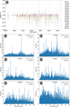 |
Fig. 6 (A) Real data from NenuFAR observations. The colour corresponds to different frequency ranges of 5 MHz. (B-G) Corresponding periodograms of the S/N of the LS power (noted S/N(LS))for seven frequency ranges averaged on a 5 MHz bandwidth: (B) [8, 13[ MHz, (C) [13, 18[ MHz, (D) [18, 23[ MHz, (E) [23, 28[ MHz, (F) [28, 33[ MHz, (G) [33, 38[ MHz. The 95% confidence level is also shown in the LS periodograms. |
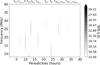 |
Fig. 7 Fig. 7. S/N of 2D LS periodogram. The Y-axis represents the observed frequencies (from 8 to 43 MHz), and the X-axis represents the LS periodicities. Periodicities of interest are indicated above the top Y-axis. |
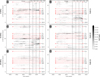 |
Fig. 8 S/N of 2D LS periodograms for six different 5-MHz frequency intervals ([8, 13[ MHz, [13, 18[ MHz, [18, 23[ MHz, [23, 28[ MHz, [28, 33[ MHz, and [33, 38[ MHz). In each panel, the Y -axis represents the LS periodicities, and the X-axis represents the calendar time (in years). The LS periodograms are calculated over a 500 day sliding window, which shifts by two days. The mean time is taken for each window, and the corresponding S/N of the LS periodogram is displayed in grey. The colour bar, thresholded to remove background noise from the periodograms, is the same for all panels. The different dashed red lines give (from top to bottom) the following periodicities: Tbeat D-J, Tbeat I-J, Tday/2, Tbeat E-J (for Europa-Jupiter), Tbeat G-J (for Ganymede-Jupiter), TJupiter, Tcomb D-J, and TJupiter/2. The vertical dotted line indicates the NenuFAR observing phase, from Early Science to Cycle 5. |
4 Summary and discussions
In this article, we analyse and demonstrate how the use of the LS periodogram is affected by a sporadic signal that is more or less regular in time, and more or less diluted with noise. The different peaks in the periodogram were analysed to determine their association with real signals.
First, a sinusoidal signal was simulated with a periodicity of T = 12.9 hours and an amplitude between −1 and 1, spanning five years. Only 2.65% of the data points were randomly retained. When the LS periodogram was applied, the highest peak was clearly located at 12.9 hours, corresponding to the input signal’s periodicity.
In the second simulation, the retained data were grouped into 125 intervals, each lasting eight hours, separated by N × 23.93 hours (N = 1,2,3,... ). The LS periodogram still showed the highest peak at 12.9 hours, but additional peaks appeared with significant power at periodicities such as 27.8 hours, 8.4 hours, and 6.2 hours. These correspond to the beat or combination periods of the input signal’s periodicity and the interval between observations.
In the third simulation, noise was introduced by adding a normal distribution to dilute the signal. This increased the noise in the LS periodogram, causing a drastic decrease in the normalised peak power. The periodogram started resembling those of real observed signals. Despite this, with a dilution factor of up to 15, the input signal’s periodicity remained easily detectable, standing out above the noise with a confidence level above 95%. Additionally, two other peaks related to the beat period and combination period between the input signal and the observation gap were observed. Even with a diluted signal, the three main peaks retained their link to the input signal, strengthening the detection.
The LS periodogram was then applied to real observations of the circular degree of polarisation of Jupiter’s radio emissions, collected with the NenuFAR radio telescope and integrated over 10 minutes and 1 MHz (Figure 7) or 5 MHz (Figure 6). It should be noted that time and frequency integration are relatively important if LS analysis is to be effective; integrating over the whole frequency band greatly dilutes the signal and decreases the S/N, and therefore it does not allow any periodicities to be detected; keeping the initial resolution (12 kHz) does not give enough weight to the signal, which is located over a wider frequency range. It is therefore necessary to produce several data sets with different integrations. We found that integrating over 1 MHz is optimal, giving a good S/N and greater detail in the 2D plot (see Figure 7), but integration over 5 MHz is sufficient to focus on the major trends (see Figure 6). Regarding the time integration, Jovian emissions studied here are often observed over several tens of minutes to several hours (see Figure 5), and periodicities of the order of an hour to tens of hours were searched in the present case. Keeping the original resolution (84 msec) is therefore not useful and would increase the time required to calculate the LS periodogram. We determined through several runs that integration over ten minutes is the most appropriate in this case.
Depending on the analysis method -either over the entire six-year interval or using a sliding window of 500 days with a two-day step- and the observed frequency range, different peaks were detected. At low frequencies, the highest peak was found at 23.93 hours, corresponding to both the sidereal day and the interval between Jupiter’s meridian transits. A smaller peak was also detected at half this period. These peaks are only visible at low frequencies for two probable reasons: (i) there are still some RFIs present in the V/I data, and these RFIs are only visible below 20 MHz during the day; (ii) only the Jovian auroral radio emissions (usually seen at <25 MHz) affect these periodicities, as they can be observed each time Jupiter is visible in the sky, while Io-induced emissions are visible only if Io is in quadrature. Four peaks were detected that are associated with Jupiter’s full- and half-rotation periods, the beat period between Jupiter and its moon Io, and half of Io’s orbital period. Four additional peaks linked to Jupiter or Io-induced emissions were detected, at the beat and combination periods between Jupiter’s and Earth’s day length, between the day and the beat period between Jupiter and its moon Io, and between half of Io’s Keplerian orbital period and the beat period between Jupiter and its moon Io. In addition, using the sliding-window technique, it enabled the detection of additional peaks at the beat period between Europa and Jupiter and at the beat period between Ganymede and Jupiter for a given period of time. The non-detection of these emissions in the 2D periodogram of Figure 7 is not a surprise; these signals are very sporadic, and the NenuFAR observations were not programmed to search for these emissions in particular, they were programmed to support the Juno mission (Bolton et al. 2017). It should be remembered that these emissions were only recently detected, either on a case-by-case basis by comparison with simulations of their occurrence (Louis et al. 2017) or via statistical methods based on 26-years of data from daily observations (Zarka et al. 2018; Jácome et al. 2022). Although emissions induced by these two moons are known to exist, their detection here may be questionable given the 1:2:4 resonance among Io, Europa, and Ganymede. Indeed, there is no filtering or reorganisation of the data before applying the LS analysis. Thus, Io’s emissions could disrupt the LS analysis, and their one-in-two or one-in-four detection could give power to the LS Jupiter-Europa or Jupiter-Ganymede beat period. However, looking at panel 8B, the S/N increase at the beat periods of Europa and Ganymede is not observed at the same time, and little-to-no signal is detected at the beat period of Io at these times, reinforcing their detection.
For the sake of completeness, this technique was also tested on a dataset covering a longer period of time and, above all, pre-catalogued (see Appendix B). To this end, the LS analysis was performed on the Nançay Decameter Array (NDA) database built by Marques et al. (2017a), which separates Io-induced from non-Io-induced emissions. Figure B.1 (top panel) shows a 2D periodogram of all the catalogued NDA data. This periodogram shows, as the one in Figure 7, S/N enhancements at typical periods (TJupiter, Tbeat I/J, TDay, TDay/2, and beat and combination periods between these different periodicities), while showing stronger S/Ns and peaks at many other beat and combination frequencies that we do not describe in detail here. As this LS analysis was done on a large dataset (26 years of data with eight hours of daily observations) of catalogued data, it shows an upper limit to what a LS analysis can provide. Finally, the middle and bottom panels of Figure B.1 show LS periodograms of Io and non-Io data, respectively. Comparing them confirms what was described above; i.e. that non-Io emissions (and therefore mainly Jupiter) are only observed below ∼25 MHz, and that the peaks at Tday and Tday/2 are mainly due to the return of the auroral Jupiter radio emissions (i.e. non-Io induced) in the observer’s sky, and not much by the Earth’s rotation period (i.e. the RFI).
Concerning the synchrotron radiation, which is briefly mentioned in Section 3, to detect the weak circularly polarised signal for this radiation the resolution of the instrument must be at least equal to half the diameter of Jupiter in order to resolve the eastern and western components of the radiation belts (and to avoid smearing). Upcoming SKA-low stations (Dewdney et al. 2022) might provide the necessary baseline to resolve this emission at low frequencies (down to 50 MHz).
These results demonstrate that the LS periodogram is a powerful tool for detecting periodic radio emissions from unevenly sampled data. It not only identifies strong signals, such as Jupiter’s auroral radio emissions and Io-induced emissions, it also detects weaker or more sporadic signals such as those linked to Europa or Ganymede.
At first glance, one might think that regular gaps in observation would weaken the analysis by introducing spurious periodic signals. While it is true that this regularity produces a peak in the periodograms (at Tday), it also creates peaks of combination or beat periods with the real signal (e.g. TDay-Jupitercomb, TDay-Jupiterbeat, T(Io-Jupiterbeat-Day)beat; see Appendix A for more details on the ratio between the S/N(LS) peaks of these different periodicities), which can be used to reinforce detections.
In our observations of Jupiter, data were often collected when Io-induced radio emissions were expected. While one might think this biases the results, this approach is consistent with our simulations (where the signal was always present) and parallels current efforts in exoplanet studies, where observations are programmed for a maximum likelihood of detecting signals, such as during quadrature phases with exoplanets (Lamy et al. 2023b) using prediction tools (e.g., ExPRES, Louis et al. 2019; PALANTIR, Mauduit et al. 2023; phase prediction, Zhang et al. 2025a).
This technique will be applied to a blind search for exo-planetary or star-planet interaction signals in NenuFAR radio telescope data. It will be useful to run it on detected radio signals (several for a single source; e.g. Zhang et al. 2023, 2025b; Zarka et al. 2025; Tasse et al. 2025) to help determine possible origins by looking at the period organisation of the detected signals. Depending on the configuration of the star-exoplanet system and the geometry of the observation, the detection of the signal (depending on the orientation of the magnetic field with respect to the observer; e.g. Lamy et al. 2023b) and the periodicities will be affected. If a signal is detected at the orbital period of the exoplanet (or at the beat period between the star and the exoplanet), this would indicate an emission produced by the SPI; if the magnetic field of the star is dipolar or axisymmetric (i.e. aligned with the rotation axis), most of the LS power will be in the exoplanet’s orbital period. On the other hand, if the magnetic field is either non-dipolar or non-axisymmetric (e.g. tilted, offset), most of the LS power will be in the beat period between the star and the exoplanet. More precisely, once the detection is done, the study of the individual bursts and in particular the variation of the maximal frequency of the emissions will inform us of the maximal magnetic-field value along the magnetic-field lines connected to the exoplanet, and therefore of the tilt, offset, and potential magnetic anomalies (Hess & Zarka 2011). A signal detected at the exoplanet’s period of rotation would suggest an auroral emission from the exoplanet itself; a signal detected at the star’s period of revolution would indicate auroral emission from the star itself; and, finally, no periodicity could point towards auroral emission from the star in the form of a hot spot (sudden stellar eruptions; e.g. Zhang et al. 2023, 2025b; Zarka et al. 2025).
Data availability
Pre-processed data from the NenuFAR Key Project 07 observations of Jupiter used in this article can be accessed at https://doi.org/10.25935/7a1s-rf17 (Louis et al. 2025b). Unprocessed NenuFAR data are available upon request to PIs of key projects. The pipeline used to create this dataset can be accessed at https://doi.org/10.5281/zenodo.15065695 (Louis et al. 2025a). The NDA dataset are available at Lamy et al. (2021) and the catalogue at Marques et al. (2017b).
Acknowledgements
C.L., A.L., P.Z., L.L. acknowledge funding from the ERC under the European Union’s Horizon 2020 research and innovation program (grant agreement N° 101020459—Exoradio, doi: 10.3030/101020459). The French authors acknowledge support from CNES and from CNRS/INSU programs of Planetology (PNP) and Heliophysics (ATST). The authors thank the anonymous referee for his meticulous work. Finally, C.L. would like to thank Q. Duchene and J. Morin for their help on getting information on ZDI and the detection limits, and E. Berriot for preliminary discussions on comparisons between periodicity detection techniques.
References
- Astropy Collaboration (Robitaille, T.P., et al.) 2013, A&A, 558, A33 [NASA ADS] [CrossRef] [EDP Sciences] [Google Scholar]
- Astropy Collaboration (Price-Whelan, A. M., et al.) 2018, AJ, 156, 123 [Google Scholar]
- Astropy Collaboration (Price-Whelan, A. M., et al.) 2022, ApJ, 935, 167 [NASA ADS] [CrossRef] [Google Scholar]
- Ben-Jaffel, L., Ballester, G. E., García Muñoz, A., et al. 2022, Nat. Astron., 6, 141 [NASA ADS] [CrossRef] [Google Scholar]
- Bigg, E. K. 1964, Nature, 203, 1008 [NASA ADS] [CrossRef] [Google Scholar]
- Bloot, S., Callingham, J. R., Vedantham, H. K., et al. 2024, A&A, 682, A170 [NASA ADS] [CrossRef] [EDP Sciences] [Google Scholar]
- Bolton, S. J., Lunine, J., Stevenson, D., et al. 2017, Space Sci. Rev., 213, 5 [CrossRef] [Google Scholar]
- Boudouma, A., Zarka, P., Magalhães, F. P., et al. 2023, in Planetary, Solar and Heliospheric Radio Emissions IX, eds. C. K. Louis, C. M. Jackman, G. Fischer, A. H. Sulaiman, & P. Zucca (Dublin: Dublin Institute for Advanced Studies and Trinity College Dublin), 103094 [Google Scholar]
- Brown, E. L., Jeffers, S. V., Marsden, S. C., et al. 2022, MNRAS, 514, 4300 [CrossRef] [Google Scholar]
- Burke, B. F., & Franklin, K. L. 1955, J. Geophys. Res., 60, 213 [NASA ADS] [CrossRef] [Google Scholar]
- Callingham, J. R., Pope, B. J. S., Feinstein, A. D., et al. 2021a, A&A, 648, A13 [EDP Sciences] [Google Scholar]
- Callingham, J. R., Vedantham, H. K., Shimwell, T. W., et al. 2021b, Nat. Astron., 5, 1233 [NASA ADS] [CrossRef] [Google Scholar]
- Callingham, J. R., Shimwell, T. W., Vedantham, H. K., et al. 2023, A&A, 670, A124 [NASA ADS] [CrossRef] [EDP Sciences] [Google Scholar]
- Callingham, J. R., Pope, B. J. S., Kavanagh, R. D., et al. 2024, Nat. Astron., 8, 1359 [NASA ADS] [CrossRef] [Google Scholar]
- Cauley, P. W., Shkolnik, E. L., Llama, J., & Lanza, A. F. 2019, Nat. Astron., 3, 1128 [NASA ADS] [CrossRef] [Google Scholar]
- Cecconi, B., Aicardi, S., & Lamy, L. 2023, Front. Astron. Space Sci., 10 [Google Scholar]
- Chen, Y. P., Zhou, G. C., Yoon, P. H., & Wu, C. S. 2002, PoP, 9, 2816 [Google Scholar]
- Collet, B., Lamy, L., Louis, C. K., et al. 2023, in Planetary, Solar and Helispheric Radio Emissions IX, eds. C. K. Louis, C. M. Jackman, G. Fischer, A. H. Sulaiman, & P. Zucca (Dublin: Dublin Institute for Advanced Studies and Trinity College Dublin) [Google Scholar]
- Collet, B., Lamy, L., Louis, C. K., et al. 2024, J. Geophys. Res. Space Phys., 129, e2024JA032422 [Google Scholar]
- Collet, B., Lamy, L., Louis, C. K., Hue, V., & Kim, T. K. 2025, Geophys. Res. Lett., 52, e2024GL114447 [Google Scholar]
- Connerney, J. E. P., Timmins, S., Oliversen, R. J., et al. 2022, J. Geophys. Res. Planets, 127, e07055 [NASA ADS] [CrossRef] [Google Scholar]
- Dewdney, P., Labate, M. G., Swart, G., et al. 2022, SKA: Design Baseline Description, Revision 2, Technical Report SKA-TEL-SKO-0001075, Square Kilometre Array (SKA), https://doi.org/10.5281/zenodo.16895574 [Google Scholar]
- Girard, J. N., Zarka, P., Tasse, C., et al. 2016, A&A, 587, A3 [NASA ADS] [CrossRef] [EDP Sciences] [Google Scholar]
- Hess, S. L. G., & Zarka, P. 2011, A&A, 531, A29 [NASA ADS] [CrossRef] [EDP Sciences] [Google Scholar]
- Hess, S., Cecconi, B., & Zarka, P. 2008, Geophys. Res. Lett., 35, L13107 [NASA ADS] [CrossRef] [Google Scholar]
- Jácome, H. R. P., Marques, M.S., Zarka, P., et al. 2022, A&A, 665, A67 [NASA ADS] [CrossRef] [EDP Sciences] [Google Scholar]
- Kao, M. M., Hallinan, G., Pineda, J. S., Stevenson, D., & Burgasser, A. 2018, ApJS, 237, 25 [NASA ADS] [CrossRef] [Google Scholar]
- Kimura, T., Tsuchiya, F., Misawa, H., et al. 2011, J. Geophys. Res. Space Phys., 116, A03204 [Google Scholar]
- Kimura, T., Lamy, L., Tao, C., et al. 2013, J. Geophys. Res. Space Phys., 118, 7019 [NASA ADS] [CrossRef] [Google Scholar]
- Kurth, W. S., Gurnett, D. A., Menietti, J. D., et al. 2011, in Planetary, Solar and Heliospheric Radio Emissions (PRE VII), eds. H. O. Rucker, W. S. Kurth, P. Louarn, & G. Fischer (Dublin: Dublin Institute for Advanced Studies and Trinity College Dublin), 75 [Google Scholar]
- Kuzmychov, O., Berdyugina, S. V., & Harrington, D. M. 2017, ApJ, 847, 60 [NASA ADS] [CrossRef] [Google Scholar]
- Lamy, L. 2017, in Planetary Radio Emissions VIII, eds. G. Fischer, G. Mann, M. Panchenko, & P. Zarka, 171 [Google Scholar]
- Lamy, L., Zarka, P., Cecconi, B., et al. 2008, J. Geophys. Res. Space Phys., 113, A07201 [NASA ADS] [Google Scholar]
- Lamy, L., Schippers, P., Zarka, P., et al. 2010, Geophys. Res. Lett., 37, L12104 [Google Scholar]
- Lamy, L., Le Gall, A., Cecconi, B., et al. 2021, Nançay Decameter Array (NDA) Jupiter Routine observation data collection (Version 1.7) [Data set], https://doi.org/10.25935/dv2f-x016 [Google Scholar]
- Lamy, L., Duchêne, A., Mauduit, E., et al. 2023a, in Planetary, Solar and Heliospheric Radio Emissions IX, eds. C. K. Louis, C. M. Jackman, G. Fischer, A. H. Sulaiman, & P. Zucca (Dublin: Dublin Institute for Advanced Studies and Trinity College Dublin), 103097 [Google Scholar]
- Lamy, L., Waters, J. E., & Louis, C. K. 2023b, in Planetary, Solar and Heliospheric Radio Emissions IX, eds. C. K. Louis, C. M. Jackman, G. Fischer, A. H. Sulaiman, & P. Zucca (Dublin: Dublin Institute for Advanced Studies and Trinity College Dublin), 103091 [Google Scholar]
- Le Queau, D., Pellat, R., & Roux, A. 1984a, Phys. Fluids., 27, 247 [Google Scholar]
- Le Queau, D., Pellat, R., & Roux, A. 1984b, J. Geophys. Res., 89, 2831 [Google Scholar]
- Lee, S.-Y., Yi, S., Lim, D., et al. 2013, J. Geophys. Res. Space Phys., 118, 7036 [Google Scholar]
- Louarn, P., Allegrini, F., McComas, D. J., et al. 2017, Geophys. Res. Lett., 44, 4439 [CrossRef] [Google Scholar]
- Louarn, P., Allegrini, F., McComas, D. J., et al. 2018, Geophys. Res. Lett., 45, 9408 [NASA ADS] [CrossRef] [Google Scholar]
- Louis, C. K., Lamy, L., Zarka, P., Cecconi, B., & Hess, S. L. G. 2017, J. Geophys. Res. Space Phys., 122, 9228 [CrossRef] [Google Scholar]
- Louis, C. K., Hess, S. L. G., Cecconi, B., et al. 2019, A&A, 627, A30 [NASA ADS] [CrossRef] [EDP Sciences] [Google Scholar]
- Louis, C. K., Zarka, P., Dabidin, K., et al. 2021, J. Geophys. Res. Space Phys., 126, e29435 [Google Scholar]
- Louis, C. K., Louarn, P., Collet, B., et al. 2023a, J. Geophys. Res. Space Phys., 128, e2023JA031985 [NASA ADS] [CrossRef] [Google Scholar]
- Louis, C. K., Smith, K. D., Jackman, C. M., et al. 2023b, in Planetary, Solar and Heliospheric Radio Emissions IX, eds. C. K. Louis, C. M. Jackman, G. Fischer, A. H. Sulaiman, & P. Zucca (Dublin: Dublin Institute for Advanced Studies and Trinity College Dublin), 103088 [Google Scholar]
- Louis, C. K., Loh, A., Zarka, P., Mauduit, E., & Girard, J. N. 2025a, A Pipeline to process NenuFAR beamformed data and calculate Lomb-Scargle Periodograms, https://doi.org/10.5281/zenodo.15078360 [Google Scholar]
- Louis, C. K., Loh, A., Zarka, P., et al. 2025b, Pre-processed data from the NenuFAR Key Project 07 observations of Jupiter (Version 1.0) [Data set], https://doi.org/10.25935/7a1s-rf17 [Google Scholar]
- Marques, M. S., Zarka, P., Echer, E., et al. 2017a, A&A, 604, A17 [NASA ADS] [CrossRef] [EDP Sciences] [Google Scholar]
- Marques, M., Zarka, P., Echer, E., et al. 2017b, Jupiter decametric radio emissions over 26 years, https://doi.org/10.26093/cds/vizier.36040017 [Google Scholar]
- Mauduit, E., Grießmeier, J. M., Zarka, P., & Turner, J. D. 2023, in Planetary, Solar and Heliospheric Radio Emissions IX, eds. C. K. Louis, C. M. Jackman, G. Fischer, A. H. Sulaiman, & P. Zucca (Dublin: Dublin Institute for Advanced Studies and Trinity College Dublin), 103092 [Google Scholar]
- Mutel, R. L., Menietti, J. D., Gurnett, D. A., et al. 2010, Geophys. Res. Lett., 37, L19105 [Google Scholar]
- Nakamura, Y., Kasaba, Y., Kimura, T., et al. 2019, Planet. Space Sci., 178, 104711 [Google Scholar]
- Pritchett, P. L. 1986a, J. Geophys. Res., 91, 13569 [NASA ADS] [CrossRef] [Google Scholar]
- Pritchett, P. L. 1986b, Phys. Fluids., 29, 2919 [Google Scholar]
- Tasse, C., Hardcastle, M., Zarka, P., et al. 2025, Nat. Astron, https://doi.org/10.1038/s41550-025-02757-7 [Google Scholar]
- Treumann, R. A. 2006, A&A, 13, 229 [Google Scholar]
- Turner, J. D., Griessmeier, J. M., Zarka, P., & Vasylieva, I. 2017, in Planetary Radio Emissions VIII, eds. G. Fischer, G. Mann, M. Panchenko, & P. Zarka, 301 [Google Scholar]
- Turner, J. D., Grießmeier, J.-M., Zarka, P., & Vasylieva, I. 2019, A&A, 624, A40 [NASA ADS] [CrossRef] [EDP Sciences] [Google Scholar]
- Turner, J. D., Zarka, P., Grießmeier, J.-M., et al. 2021, A&A, 645, A59 [NASA ADS] [CrossRef] [EDP Sciences] [Google Scholar]
- Turner, J. D., Zarka, P., Grießmeier, J. M., et al. 2023, in Planetary, Solar and Heliospheric Radio Emissions IX, eds. C. K. Louis, C. M. Jackman, G. Fischer, A. H. Sulaiman, & P. Zucca (Dublin: Dublin Institute for Advanced Studies and Trinity College Dublin), 04048 [Google Scholar]
- Turner, J. D., Grießmeier, J.-M., Zarka, P., Zhang, X., & Mauduit, E. 2024, A&A, 688, A66 [NASA ADS] [CrossRef] [EDP Sciences] [Google Scholar]
- VanderPlas, J. T. 2018, ApJS, 236, 16 [Google Scholar]
- VanderPlas, J. T., & Ivezic, Z. 2015, ApJ, 812, 18 [NASA ADS] [CrossRef] [Google Scholar]
- VanderPlas, J., Connolly, A. J., Ivezic, Z., & Gray, A. 2012, in Proceedings of Conference on Intelligent Data Understanding (CIDU), 47 [Google Scholar]
- Vasylieva, I. 2015, Theses, Paris Observatory, France, https://theses.hal.science/tel-01246634v1 [Google Scholar]
- Vedantham, H. K., Callingham, J. R., Shimwell, T. W., et al. 2020, Nat. Astron., 4, 577 [Google Scholar]
- Vedantham, H. K., Dupuy, T. J., Evans, E. L., et al. 2023, A&A, 675, L6 [NASA ADS] [CrossRef] [EDP Sciences] [Google Scholar]
- Waters, J. E., Jackman, C. M., Whiter, D. K., et al. 2022, J. Geophys. Res. Space Phys., 127, e30449 [Google Scholar]
- Wu, C. S. 1985, Space Sci. Rev., 41, 215 [NASA ADS] [CrossRef] [Google Scholar]
- Wu, C. S., & Lee, L. C. 1979, ApJ, 230, 621 [Google Scholar]
- Zakharenko, V. V., Vasylieva, I. Y., Konovalenko, A. A., et al. 2013, MNRAS, 431, 3624 [NASA ADS] [CrossRef] [Google Scholar]
- Zarka, P. 1998, J. Geophys. Res., 103, 20159 [Google Scholar]
- Zarka, P., Queinnec, J., & Crary, F. J. 2001, Planet. Space Sci., 49, 1137 [NASA ADS] [CrossRef] [Google Scholar]
- Zarka, P., Marques, M. S., Louis, C., et al. 2017, in Planetary Radio Emissions VIII, eds. G. Fischer, G. Mann, M. Panchenko, & P. Zarka, 45 [Google Scholar]
- Zarka, P., Marques, M. S., Louis, C., et al. 2018, A&A, 618, A84 [NASA ADS] [CrossRef] [EDP Sciences] [Google Scholar]
- Zarka, P., Denis, L., Tagger, M., et al. 2020, in URSI General Assembly and Scientific Symposium (URSI GASS) [Google Scholar]
- Zarka, P., Magalhaes, F. P., Marques, M. S., et al. 2021, J. Geophys. Res. Space Phys., 126, e29780 [NASA ADS] [CrossRef] [Google Scholar]
- Zarka, P., Louis, C. K., Zhang, J., et al. 2025, A&A, 695, A95 [NASA ADS] [CrossRef] [EDP Sciences] [Google Scholar]
- Zhang, J., Tian, H., Zarka, P., et al. 2023, ApJ, 953, 65 [NASA ADS] [CrossRef] [Google Scholar]
- Zhang, X., Zarka, P., Girard, J. N., et al. 2025a, A&A, 700, A140 [NASA ADS] [CrossRef] [EDP Sciences] [Google Scholar]
- Zhang, J., Tian, H., Bellotti, S., et al. 2025b, Sci. Adv., 11, eadw6116 [Google Scholar]
Appendix A Evolution of the Lomb-Scargle Periodogram as a Function of the Number of Samples
This appendix describes the evolution of the signal-to-noise Ratio (S/N) of the Lomb-Scargle (LS) Periodogram -denoted S∕N(LS)- as a function of the number of samples N included in the LS analysis. For each LS periodogram, the S∕N(LS) is calculated as S/N(LSN) = LSN/standard deviation (LSN). Figure A.1 shows the evolution for the simulated signal (diluted into noise by a factor K = 8). One can see in the top panel that it takes N ≃ 20 samples for the maximal peak in the LS periodogram to stabilize along the value of Tsine. Note that for a dilution factor K = 15 (as in Figure 4), it takes N ≃ 55 samples, and for a dilution factor K = 2, it takes N = 5 samples. In the bottom panel one can see the evolution of the S/N(LS) of the associated peak as a function of the number of samples included in the LS analysis. It is observed that the S/N(LS) evolves as the square root of the number of samples (red curve). The black dashed lines highlight the sample number N = 170 for later comparison with the S/N(LS) evolution of the real data).
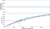 |
Fig. A.1 Evolution as a function of the number of simulated observation samples inserted into the LS analysis of (top panel) the value of the maximum peak of the LS periodogram (in hours) and (bottom panel) of the S/N (of the LS periodogram) of the associated peak in the LS. The red curve is a simple fit y = a × √(x) + b, with x the number of samples, a = 5.188 and b = −14.545. Here the simulated signal is diluted into noise, with a standard deviation σnormal distribution = K × σsine with K = 8.. The black dashed lines highlight sample N = 170 corresponding to the number of observation samples in the real data (see Figure A.2). |
Figure A.2 displays the same as Figure A.1 but for the real data. The different colors display different periodicities (see caption). The “Period of Max S/N(LS)” is calculated for each periodicities at ±2 hours around the expected periodicity of interest (grey dashed-lines). Depending on the periodicity studied, stability in the location of the Max S/N(LS) begins to be achieved from N ≳ 15-20 (TDay-Jup-beat, TJup, TDay), N ≳ 45 (TIo-Jup), N ≳ 80 (TDay-Jup-comb), or even N ≳ 110 (TIo/2). There is, of course, more variation than for the simulated signal, due to the beaming and the viewing effect of the radio emissions. Concerning the S/N(LS), one can see that, as for the simulated signal, it evolves as the square root of the number of samples.
The bottom panel of Figure A.2 allows for a more quantitative comparison of the S/N(LS) of the different periods. We will focus only on the last point of the distributions (N = 170), corresponding to the values displayed in Figure 7. The peak associated with TJupiter has an S/N(LS) = 47.4; for TJupiter/2: 9.0; for TJupiter-Iobeat: 30.6; for TIo: 3.8 (not shown here); for TIo/2 : 18.5; for TDay: 22.4; for TDay/2: 15.3 (not shown here); and for the beat and combination period: TJupiter-Io beat — Io/2beat : 4.4 (not shown here); TJupiter-Daybeat: 25.2; TJupiter-Daycomb : 27.2; T(Io-Jupiterbeat-Day)beat : 10.2 (not shown here).
The fact that the two highest S/N(LS) values are for TJupiter and TJupiter-Iobeat highlights two things: (i) radio emissions are produced by Jupiter itself and by the interaction between Jupiter and its moon Io; (ii) the S/N(LS) of TJupiter-Iobeat is higher than the S/N(LS) of TIo, proving that Jupiter’s magnetic field is not axisymmetric. This is further highlighted by the S/N(LS) values higher for TIo/2 than for TIo.
Due to the high S/N(LS) value for TDay, S/N(LS) of beat and/or combination periods between the three highest periods and TDay are also detected.
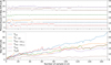 |
Fig. A.2 Evolution as a function of the number of observation samples inserted into the LS analysis of (top panel) the values of the maximum peaks of the LS periodogram (in hours) -sought within ±2 hours of the theoretical value (grey lines)- and (bottom panel) of the S/N (of the LS periodogram) of the associated peak in the LS. The different colors correspond to the different periodicities detected in the LS periodogram: blue: TJupiter; orange: TIo-Jupiterbeat; green: TDay-Jupiterbeat; red: TDay-Jupitercombination; purple: TDay; brown: TIo/2. |
Appendix B Lomb-Scargle Analysis of the Marques et al. (2017a) Nançay Decameter Array Catalogue
In this appendix are detailled the results of the LS analysis of the Marques et al. (2017a) Nançay Decameter Array Catalogue, ranging from January 1990 to April 2020. In this catalogue, all observed Jovian emissions, were labeled with respect to their time-frequency morphology, their dominant circular polarization and maximum frequency. They are separated into Io and non-Io induced radio emissions. Figure B.1 displays the S/N of the 2D LS Periodograms for all emissions (top panel) and separated into Io-induced (middle panel) and non-Io emissions (bottom panel). For Io-induced emissions, high S/N is clearly visible at all periodicities related to Io (TIo, TIo/2, Tbeat Io/2-IJ, Tbeat D-IJ, Tbeat IJ). For non-Io-induced emissions, high S/N is visible for periodicities linked to either Jupiter (TJ) or the day (TD, TD/2), or combinations of both (TbeatDJ, Tcomb DJ). These periodicities are detected at lower observed frequencies (up to 26 MHz only) than Io-induced emissions, due to magnetic field topology. No clear peak is visible for Europa and Ganymede, which is also not surprising as they are not that often visible in the data, even if they were statistically detected using this catalogue (Zarka et al. 2017, 2018; Jácome et al. 2022), but after having been sorted by position of the moons as a function of the observer.
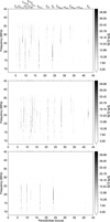 |
Fig. B.1 Signal to Noise ratio of the 2D LS Periodogram for (top panel) all emissions, (middle panel) Io-induced emissions, (bottom panel) non-Io emissions. The Y-axis represents the observed frequencies (from 8 to 45 MHz); the X-axis represents the LS periodicities. Periodicities of interest are indicated above the top y-axis. |
All Tables
Possible fundamental, beat, and combination periods that could be expected due to the sine, observed, and gap periods in our simulated signal.
Possible fundamental, beat, and combination periods that could be expected due to the rotation periods of Jupiter and its moons, and the day/observation periodicity.
All Figures
|
Fig. 1 (Left) Randomly spaced sinusoidal wave with period Tsine = 12.90 h. Only a few days of the entire five-year interval are shown in order to show the sinusoidal signal clearly. (Right) Corresponding LS periodogram. The 95% confidence level (based on a randomisation test) is indicated for the LS periodogram. It is very low in this case as only signal is given (no noise). |
| In the text | |
|
Fig. 2 (Left) Semi-regularly spaced sinusoidal wave with period Tsine = 12.90 h. The samples are gathered into 125 intervals of eight hours, spaced by N × 23.93 hours (with N = 1,2,3,4,...). (Right) Corresponding LS periodogram. The 95% confidence level is also indicated. It is also very low in this case as only a signal is given (no noise). |
| In the text | |
|
Fig. 3 Same as Figure 2, but with all values of the sinusoid at 1 in order to show the effect of the windowing on the LS periodogram. The 95% confidence level is also indicated. As all values are saturated to 1, randomly shuffling the values does not change the LS analysis, and the 95% confidence level is at the values of the highest peaks (due to the sidereal periodicity at N × 23.93 hours). |
| In the text | |
|
Fig. 4 (Left panel) Semi-regularly spaced sinusoidal wave with period Tsine = 12.90 h (light blue), normal distribution with a standard deviation of σ = K × σsin with K = 15 (light grey), and combined signal with higher signal-to-noise ratio (red points). The samples are gathered into 125 intervals of eight hours spaced by N × 23.93 hours. (Right panel) Corresponding LS periodogram. The 95% confidence level is also shown in the LS periodogram. |
| In the text | |
|
Fig. 5 Typical NenuFAR ‘time (UTC) versus frequency (in MHz) spectrogram, of Jupiter signal. (Top panel) Stokes I with data preprocessing applied (see text). (Bottom panel) Ratio between Stokes V and Stokes I showing the degree of circular polarisation. |
| In the text | |
|
Fig. 6 (A) Real data from NenuFAR observations. The colour corresponds to different frequency ranges of 5 MHz. (B-G) Corresponding periodograms of the S/N of the LS power (noted S/N(LS))for seven frequency ranges averaged on a 5 MHz bandwidth: (B) [8, 13[ MHz, (C) [13, 18[ MHz, (D) [18, 23[ MHz, (E) [23, 28[ MHz, (F) [28, 33[ MHz, (G) [33, 38[ MHz. The 95% confidence level is also shown in the LS periodograms. |
| In the text | |
|
Fig. 7 Fig. 7. S/N of 2D LS periodogram. The Y-axis represents the observed frequencies (from 8 to 43 MHz), and the X-axis represents the LS periodicities. Periodicities of interest are indicated above the top Y-axis. |
| In the text | |
|
Fig. 8 S/N of 2D LS periodograms for six different 5-MHz frequency intervals ([8, 13[ MHz, [13, 18[ MHz, [18, 23[ MHz, [23, 28[ MHz, [28, 33[ MHz, and [33, 38[ MHz). In each panel, the Y -axis represents the LS periodicities, and the X-axis represents the calendar time (in years). The LS periodograms are calculated over a 500 day sliding window, which shifts by two days. The mean time is taken for each window, and the corresponding S/N of the LS periodogram is displayed in grey. The colour bar, thresholded to remove background noise from the periodograms, is the same for all panels. The different dashed red lines give (from top to bottom) the following periodicities: Tbeat D-J, Tbeat I-J, Tday/2, Tbeat E-J (for Europa-Jupiter), Tbeat G-J (for Ganymede-Jupiter), TJupiter, Tcomb D-J, and TJupiter/2. The vertical dotted line indicates the NenuFAR observing phase, from Early Science to Cycle 5. |
| In the text | |
|
Fig. A.1 Evolution as a function of the number of simulated observation samples inserted into the LS analysis of (top panel) the value of the maximum peak of the LS periodogram (in hours) and (bottom panel) of the S/N (of the LS periodogram) of the associated peak in the LS. The red curve is a simple fit y = a × √(x) + b, with x the number of samples, a = 5.188 and b = −14.545. Here the simulated signal is diluted into noise, with a standard deviation σnormal distribution = K × σsine with K = 8.. The black dashed lines highlight sample N = 170 corresponding to the number of observation samples in the real data (see Figure A.2). |
| In the text | |
|
Fig. A.2 Evolution as a function of the number of observation samples inserted into the LS analysis of (top panel) the values of the maximum peaks of the LS periodogram (in hours) -sought within ±2 hours of the theoretical value (grey lines)- and (bottom panel) of the S/N (of the LS periodogram) of the associated peak in the LS. The different colors correspond to the different periodicities detected in the LS periodogram: blue: TJupiter; orange: TIo-Jupiterbeat; green: TDay-Jupiterbeat; red: TDay-Jupitercombination; purple: TDay; brown: TIo/2. |
| In the text | |
|
Fig. B.1 Signal to Noise ratio of the 2D LS Periodogram for (top panel) all emissions, (middle panel) Io-induced emissions, (bottom panel) non-Io emissions. The Y-axis represents the observed frequencies (from 8 to 45 MHz); the X-axis represents the LS periodicities. Periodicities of interest are indicated above the top y-axis. |
| In the text | |
Current usage metrics show cumulative count of Article Views (full-text article views including HTML views, PDF and ePub downloads, according to the available data) and Abstracts Views on Vision4Press platform.
Data correspond to usage on the plateform after 2015. The current usage metrics is available 48-96 hours after online publication and is updated daily on week days.
Initial download of the metrics may take a while.