| Issue |
A&A
Volume 707, March 2026
|
|
|---|---|---|
| Article Number | A35 | |
| Number of page(s) | 10 | |
| Section | Astrophysical processes | |
| DOI | https://doi.org/10.1051/0004-6361/202555277 | |
| Published online | 25 February 2026 | |
Lensing of hot spots in Kerr space-time
An empirical relation for black hole spin estimation
1
Department of Astrophysics/IMAPP, Radboud University P.O. Box 9010 6500 GL Nijmegen, The Netherlands
2
Center for Astrophysics | Harvard & Smithsonian 60 Garden Street Cambridge MA 02138, USA
3
Black Hole Initiative at Harvard University 20 Garden Street Cambridge MA 02138, USA
★ Corresponding author: This email address is being protected from spambots. You need JavaScript enabled to view it.
Received:
23
April
2025
Accepted:
29
December
2025
Abstract
Context. Sagittarius A* (Sgr A*) exhibits frequent flaring activity across the electromagnetic spectrum that is often associated with a localized region of strong emission known as a hot spot.
Aims. We aim to establish an empirical relationship linking key parameters of this phenomenon – emission radius, inclination, and black hole spin – to the observed angle difference between the primary and secondary image (ΔPA) that an interferometric array could resolve.
Methods. Using the numerical radiative transfer code ipole, we generated a library of more than 900 models with varying system parameters and computed the position angle difference on the sky between the primary and secondary images of the hot spot. The key assumptions are equatorial and circular orbits.
Results. For these models we find that the average ΔPA over a full period is insensitive to inclination. This result significantly simplifies potential spin measurements, which might otherwise depend strongly on inclination. Additionally, we derived a relation connecting spin to ΔPA, given the period and emission radius of the hot spot, with an accuracy of better than 5° in most cases. Finally, we present a mock observation to showcase the potential of this relation for spin inference.
Conclusions. Our results provide a novel approach for black hole spin measurements using high-resolution observations, such as future movies of Sgr A* obtained with the Event Horizon Telescope, the next-generation Event Horizon Telescope, and the Black Hole Explorer. Although discrepancies will likely arise in the general case (lifting model assumptions), the methodology is sound, and easily extendable.
Key words: black hole physics / gravitational lensing: strong / methods: analytical / methods: numerical / techniques: high angular resolution / Galaxy: center
© The Authors 2026
 Open Access article, published by EDP Sciences, under the terms of the Creative Commons Attribution License (https://creativecommons.org/licenses/by/4.0), which permits unrestricted use, distribution, and reproduction in any medium, provided the original work is properly cited.
This article is published in open access under the Subscribe to Open model. This email address is being protected from spambots. You need JavaScript enabled to view it. to support open access publication.
1. Introduction
The Event Horizon Telescope (EHT) has produced images of the supermassive black holes Messier 87* (hereafter M87*) and Sagittarius A* (hereafter Sgr A*), providing an unprecedented laboratory for testing accretion models and studying the effects of light propagation in general relativity (EHTC 2019b, 2022b, 2024a). Additionally, observations by the GRAVITY collaboration have constrained the mass of Sgr A* to M = 4.3 × 10⁶ M⊙ ± 0.25% (GRAVITY Collaboration 2022), establishing a crucial reference for event-horizon-scale tests of space-time, such as black hole spin measurements and potential deviations from general relativity.
A major challenge when performing precision space-time tests from black hole images is disentangling the plasma effects of accretion from the pure general relativity signatures of the underlying space-time. The combination of finite observational resolution, strong interstellar scattering along the Galactic Center line of sight, and the short dynamical timescale of Sgr A* (approximately 30 minutes at the innermost stable circular orbit for a Schwarzschild black hole) makes this separation particularly difficult. Consequently, any attempt to estimate the dimensionless spin parameter, a* = Jc/GM2, must rely on identifying a signature in one of the less plasma-dependent observables.
Among the most distinctive features of black hole space-times is their ability to trap photons in unstable yet bound orbits (Bardeen et al. 1972). In the case of a Kerr black hole, the shape and size of these orbits depend solely on the black hole’s mass and spin. The region where these bound orbits reside is known as the photon sphere. As photons escape these unstable orbits and reach a distant observer, they appear as a narrow “photon ring” on the image plane; they can asymptotically approach the so-called critical curve depending on the number of windings the photon undergoes around the black hole before arrival. These features have been extensively studied in recent works, both theoretically (Claudel et al. 2001; Johannsen & Psaltis 2010; Gralla et al. 2019; Gralla & Lupsasca 2020; Kocherlakota et al. 2024) and in connection with observations (Johnson et al. 2020; Gralla et al. 2020; Wong 2021; Zhou et al. 2025; Zhang et al. 2025). The Black Hole Explorer (BHEX) mission (Johnson et al. 2024; Lupsasca et al. 2024; Galison et al. 2024) has set the precise measurement of the photon ring as a key science goal.
In this work we focused on a specific effect of black hole lensing: the secondary images of localized sources, or “hot spots”, a subcategory of photon rings. Unlike a full ring, the secondary image remains compact and forms a crescent. This provides a unique opportunity to distinguish direct from lensed photons in the image, enabling the application of the mathematical framework developed for null geodesics. We studied two key observational effects: the time lag between primary and secondary photons (n = 0 and n = 1) and the difference in position angle on the screen (ΔPA), with a particular focus on the latter. Specifically, we derived a new analytic approximation for calculating δPA (where δPA denotes the analytic estimate, while ΔPA refers to the observational measurement), propose a method for disentangling the inclination angle (i) from ΔPA measurements, and establish an empirical relation connecting ΔPA to black hole spin. Definitions of the different terms used in this paper for ΔPA are provided in Table 1.
Descriptions of various notations used in the analysis.
This method is entirely achromatic, as it depends solely on the geometric properties of the system rather than specific emission mechanisms. While the appearance of a single hot spot may differ between, for example, radio and near-infrared (NIR) wavelengths, the geometric relations underlying our method remain valid in both regimes.
Observations of Sgr A* support the presence of emission from localized regions, as the source exhibits regular flaring events across the electromagnetic spectrum on characteristic timescales of ∼20 hours. During these events, NIR radiation can increase by 1–2 orders of magnitude (GRAVITY Collaboration 2020a), while the brightest X-ray flares reach peaks of ∼600 times the quiescent state (Haggard et al. 2019). Additionally, GRAVITY has detected astrometric motion of the Sgr A* brightness centroid and polarimetric signatures associated with flares (GRAVITY Collaboration 2018, 2023). At radio frequencies, observations with the Atacama Large Millimeter/submillimeter Array (ALMA) have been used to link similar physical effects to corresponding signatures in the light curves of linear polarization (Wielgus et al. 2022a,b; EHTC 2022c). Proposed next-generation improvements to the EHT have specifically targeted improved dynamical imaging sensitivity for the Galactic Center due to the presence of these rapidly evolving events (Doeleman et al. 2023).
Numerous studies have modeled this localized emission (e.g., Broderick & Loeb 2006; Trippe et al. 2007; Hamaus et al. 2009; Tiede et al. 2020; Gelles et al. 2021; Vos et al. 2022; Vincent et al. 2024), and some have sought to connect simulations to observations for model classification (GRAVITY Collaboration 2020b,c; Ball et al. 2021; Aimar et al. 2023; Yfantis et al. 2024a,b; Antonopoulou & Nathanail 2024). As these models increasingly reproduce observational data, a stronger theoretical foundation becomes essential.
The broader concept of hot spots has been linked to physical processes in magnetically arrested disks (MADs; Narayan et al. 2003), which exhibit flux eruption events resembling the flaring activity of Sgr A* (Dexter et al. 2020; Scepi et al. 2022). These events can generate flux tubes – evacuated regions in the accretion flow where electrons become highly accelerated and heated via magnetic reconnection while traveling in strong vertical magnetic fields (Porth et al. 2021; Ripperda et al. 2022). Simulations by Najafi-Ziyazi et al. (2024) suggest that such structures produce signatures consistent with observations. As MADs have sub-Keplerian orbital profiles (Begelman et al. 2022; Conroy et al. 2023), the hot spots from flux eruptions should also appear sub-Keplerian. We expect such phenomena to be most prominent in the submillimeter regime, as was shown in Yfantis et al. (2024b), where a sub-Keplerian velocity for the hot spot was strongly favored from the fitting of ALMA data. In this case we would also expect the bulk of the emission to come from the equatorial plane, since the eruptions are stronger there. Our analysis focuses more on this scenario because equatorial orbits are simpler, but also because all the near-term future experiments capable of imaging in the required resolution are in the radio regime.
Another possible explanation is the formation of plasmoids via magnetic reconnection in magnetized disks (e.g., Ripperda et al. 2020; Aimar et al. 2023; Vos et al. 2024). In this case the modeling could get more complicated, with off-equatorial orbits (spiraling inward or outward) and modular velocities, as plasmoids can detach from the bulk of the disk much more easily. These effects cannot be expressed in this analysis and could significantly impact the observables. Notably though, plasmoids are expected mostly in the NIR and higher frequencies, with velocities above the Keplerian limit, differentiating them from the simpler case. In the future we plan to extend the method to include all this rich phenomenology.
An alternative phenomenon that could appear as bright “spots” are the so-called shock waves (appearing as spiral arms), as shown in Conroy et al. (2023). They are known to reside in the equatorial plane, but it is not clear whether they are strong enough that their secondary imprint would survive.
Lastly, it should be possible for two bright spots to appear simultaneously, although it is not clear at what cadence. Regardless, we could use various gauges to differentiate this from the case of a secondary image, such as the time delay between the appearance of the two images, the flux difference, and their orbital properties.
Given the growing scientific progress in both observational and modeling efforts, we anticipate that a direct image or time-resolved movie of a secondary image will become a reality in the near future. In this paper we present a straightforward and computationally efficient approach to interpreting such observations – contrasting with the full analytic treatment of photon rings – with the goal of constraining black hole spin. To this end, we have constructed a library of over 900 models with varying key system parameters: the spot’s orbital radius (rhs), the orbital velocity, the black hole spin (a*), and the inclination angle (i).
In Sect. 2 we summarize the key mathematical results from previous studies. In Sect. 3 we present our numerical scheme and the model library we used to study the problem. In Sect. 4 we introduce our intermediate findings: a simple and highly accurate (sub-degree) approximation for δPA0 → 1, (as opposed to the n → ∞ that is typically considered), along with a simplified formula that has a growing deviation with spin from the sub-degree level up to 5° for a* = 0.99. We then show that the mean value of ΔPA over a full orbit of the hot spot is insensitive to i, similar to recent results in Walia et al. (2025). This result favors simple analyses of average deflections, removing the notion of a time-dependent orbital phase and the observer’s inclination and position angle in downstream fitting. Lastly, we introduce an empirical relation derived from our model library and evaluate its accuracy in reproducing simulation results. We then apply this relation to three sets of mock observations, incorporating reasonable uncertainties for ΔPA, orbital period (P), and rhs. We show that in the case of observations that align with our simulation assumptions, our method can constrain the black hole spin to ±0.3 at the 2σ confidence level, but this fitting should be mainly viewed as a proof of concept; a dedicated fitting analysis should be performed in the future. In Sect. 5 we conclude by discussing the implications and potential limitations of this approach for future observations.
2. Mathematical prior
The goal of this section is to provide a short summary of the mathematical background governing the effects of lensing around black holes. We provide this information as a means for comparison and as a natural path toward an empirical relation that stems from simulations and which incorporates the equations presented here.
We used Boyer-Lindquist coordinates (t, r, θ, ϕ) and natural units, i.e., G = c = M = 1, so that both time and distance are measured in [M]. The line element describing the space-time is
 (1)
(1)
where a* is the dimensionless angular momentum per unit mass and
 (2)
(2)
We considered a stationary hot spot and show solutions for two quantities: the time lapse (δt) between two subsequent images (n, n+1) and the difference in their position angle on the sky (δPA) for an observer at infinity, on the symmetry axis. The solution holds only for n → ∞, implying that the parameters are evaluated at rcrit. In this paper we omit the complete solution, which contains various steps and different cases; it can be found in numerous papers (e.g., Beckwith & Done 2005; Gralla & Lupsasca 2020; Wong 2021). Instead we provide the solutions (similarly to Gralla & Lupsasca 2020) as
![Mathematical equation: $$ \begin{aligned} \delta t&= \frac{2}{\sqrt{\tilde{b}^2 - a_*^2}} \Bigg [\tilde{r}_0^2 \left( \frac{\tilde{r}_0 + 3}{\tilde{r}_0 - 1} \right) K\left( \frac{a_*^2}{a_*^2 - \tilde{b}^2} \right) \nonumber \\&\qquad - 2a_*^2 E^{\prime }\left( \frac{a_*^2}{a_*^2 - \tilde{b}^2} \right)\Bigg ] \end{aligned} $$](/articles/aa/full_html/2026/03/aa55277-25/aa55277-25-eq3.gif) (3)
(3)
and
 (4)
(4)
where
![Mathematical equation: $$ \begin{aligned} \tilde{r}_0 = 1 + 2\sqrt{1 - \frac{a_*^2}{3}} \cos \left[ \frac{1}{3} \arccos \left( \frac{1 - a_*^2}{\left(1 - \frac{a_*^2}{3}\right)^{3/2}} \right) \right] \end{aligned} $$](/articles/aa/full_html/2026/03/aa55277-25/aa55277-25-eq5.gif) (5)
(5)
is the critical radius, denoting the bound photon orbit for the face-on observer (i = 0°). The tilde on the rest of the parameters indicates that they are calculated on the critical radius. Then  , the apparent critical curve on an observer’s screen in units of M, is given by
![Mathematical equation: $$ \begin{aligned} \tilde{b} = \sqrt{\frac{\tilde{r}_0^3}{a_*^2} \left[ \frac{4 \Delta (\tilde{r}_0)}{(\tilde{r}_0 - 1)^2} - \tilde{r}_0 \right] + a_*^2}. \end{aligned} $$](/articles/aa/full_html/2026/03/aa55277-25/aa55277-25-eq7.gif) (6)
(6)
Lastly, K and E′, in Eqs. (3) and (4), represent the first and second complete elliptical integrals respectively, which can be found in math libraries, such as scipy.
For the case of a moving hot spot there is an extra degree of complexity, since the spot changes position while the photons move to the secondary image, resulting in a necessary correction for δPA (Eq. (4)). In the simplest case of a circular orbit on the equator it is given by
 (7)
(7)
where Ω is the angular velocity of the spot.
As stated, and further demonstrated in Appendix A, these equations describe the problem only for higher-order images (n → ∞). In this paper, however, we are interested in the secondary image (n = 1), so we need to quantify how much the solution deviates in this case. To our knowledge, there is no published solution for such a case; hence, we present a heuristic approximation in Sect. 4.
3. Numerical method
In this section we describe our numerical setup, built inside the general relativistic radiative transfer code ipole (Mościbrodzka & Gammie 2018). We simulated emission from a moving hot spot, closely resembling that implemented in Yfantis et al. (2024a,b). The hot spot lives in circular orbits on the equatorial plane (mostly expected in radio flares), and it has a Gaussian profile peaking at the center for its key parameters: number density (ne), electron temperature (Θe) and magnetic field strength (Bfield). Its size is dictated by the number density that has a 1σ radius of 1.5M and then a steep cutoff, creating a crisp spot size. While the spot model is defined in Boyer–Lindquist coordinates, the ray-tracing of photons is done in Kerr-Schild coordinates. The resolution is set at 256 × 256 pixels.
Our library consists of models with different values for a variety of parameters (rhs, Ωcoef, i, and a*), where rhs is the distance of the spot from the center of the black hole and the Ωcoef parameter controls the orbital velocity as
 (8)
(8)
The Ωcoef parameter provides a straightforward way to simulate sub-Keplerian orbits, highly expected in MADs, or even slower orbits associated with spiral shock waves. Appendix A provides proof that Ωcoef maps correctly to the velocity in the image domain. The parameter grid is summarized in Table 2.
Parameter values in our simulated library.
During the simulation we recorded values of the centroids of the two images, and we masked all contributions to light rays from n > 1. A simulation that includes the n = 2 image, showcasing that its contribution is completely negligible, is presented in Appendix A. Given the centroids, we defined ΔPA as
 (9)
(9)
where Xcen, Ycen and Xcen2, Ycen2 refer to the centroid of total intensity of primary and secondary images, respectively. It is worth mentioning that the correct ΔPA of a moving source can only be estimated using the slow light approach and that is what we did throughout the study. Using the fast light approximation, the second term of Eq. (7) cannot be manifested, so it is effectively a stationary hot spot, leading to large deviations1.
We also measured the arrival time of all photons to the observer, which allowed us to calculate the maximum time difference (Δt) between the primary and secondary image as the difference between the first and last photon to reach. In Fig. 1 we present two example snapshots from the simulation domain with different parameters. The imaging happens after the secondary image has appeared, meaning 5 − 15 minutes after the hot spot has emerged. The middle and right panels display the evolution of ΔPA and Δt over a full orbit. ΔPA is calculated as the angle starting at n = 0 and ending at n = 1, counterclockwise (see Fig. 1), while Δt as the difference in time between the last photon from n = 0 and the first from n = 1. Both quantities exhibit significant variation with increasing inclination, highlighting the need for a method for disentangling inclination effects from other influences. This is presented in Sect. 4.
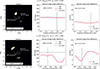 |
Fig. 1. Left: Snapshot from a hot spot movie, with resolution 256 × 256 (as in the entire library), where ΔPA is calculated from the primary to the secondary counterclockwise. Middle: Curve of ΔPA measurement with respect to time for a full period. Right: Time lag (difference in arrival times) between the first and second image. The gray vertical line in the right panels denotes the snapshot’s time in the left panels. |
4. Results
This section includes two intermediate results necessary for the construction of an empirical relation: (1) an analytic approximation for δPA0 → 1 and (2) the independence of the mean ΔPA (from a full period) with respect to inclination, similarly to the independence of the median value shown in Walia et al. (2025). Table 1 summarizes the notation of the approximations discussed here. Next we present our empirical relation that covers shortcomings from the analytic relations in order to be used as a means of inference, and lastly we show three examples of its application using mock observations of ΔPA.
4.1. Insightful analytic approximations for δPAn → 1
To address this problem, we created three models with spin parameters a* = 0, 0.5, 0.95, a smaller spot size (spot radius of 1 M), and a higher resolution (1024 × 1024 pixels). The spot is stationary and rhs is set to the critical radius for all models.
First we tested the simulation results against the δPA solution. While both methods give ΔPA = 180° for the non-spinning case, for a* = 0.5, 0.95 the analytic solution gives δPA = 216° ,263° while the simulations produce ΔPA = 198° ,218°, respectively. The reason is that the trajectories are sufficiently different for n = 0 and n = 1 that the critical parameters do not apply exactly. Thus, the complete integral (K) in Eq. (4) should be calculated as incomplete instead (Kinc). These are connected via
 (10)
(10)
where the argument in Kinc is an angle in the first part and the calculated quantity in the second. So for π/2 the incomplete becomes complete.
Via trial and error, we found that the correct angle for an incomplete integral to account for the primary-secondary (0 → 1) image solution (δPA0 → 1) is π/(π + a* + 0.3) such that
 (11)
(11)
The reason behind the a* dependence inside Kinc is that the deviation of the two formulas (δPA, δPA0 → 1) increases for high spins, as the photons are traveling a larger angle (δPA increases with increasing spin), and that needs to be accounted for. Another effective and significantly simpler way to calculate the deviation in δPA0 → 1 is by taking the expression for δPA (Eq. (4)) and removing the factor of 2 from the second term. We call this δPAf2, 0 → 1, and it is given as
 (12)
(12)
This works nearly exactly (sub-degree deviations) for spins up to ∼0.75 with deviations of just a couple degrees above that (5° for a* = 0.99). A naive but perhaps useful intuition for this approximation is that the n = 0 photons do not feel the twist of the space-time in their way in, only as they move toward the back of the black hole, and so the deflection between n = 1 and n = 0 is only half of the effect in the universal regime.
Despite these simplifications, the analytic problem remains challenging due to two key generalizations: the motion of the hot spot and the treatment of a general emission radius rhs, which is not fixed at the critical radius. We therefore proceeded with a broad numerical parameter study to identify a simpler empirical relation.
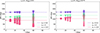 |
Fig. 2. Distribution (violins) of ΔPA values during a full period for different inclination values. The crosses denote the average values per period and the dashed lines the value at i = 0° for a fixed a*. |
4.2. Inclination dependence
To study the variations in ΔPA with inclination, we created distributions (violins) of all ΔPA values, sampled every dt = 5M over a full period, for various models. These are shown in Fig. 2, where the models are characterized by two fixed parameter sets (rhs = 4, 8 and Ωcoef = 0.5, 0.75), three spin values (a* = −0.9, 0, 0.9), and five inclination angles in the range [0, 60]. The two parameter sets (rhs, Ωcoef) are shown in separate panels, while all spin values are overlaid within each panel. The vertical axis represents ΔPA, and the horizontal axis denotes the inclination angle.
The distributions shown in Fig. 2 exhibit significant variations in both ΔPA values and their shapes depending on the parameters. However, a clear pattern emerges: the mean ΔPA for each model, marked by crosses and connected with dashed lines, remains nearly constant across inclinations. This holds especially well for inclinations up to 30° and for larger values of rhs, like in rhs = 8, where all average ΔPAs are within one degree. Even in the case of rhs = 4, the deviation at i = 60° from i = 0° is 5°. In the case of Sgr A* inclination is constrained by various observations to be i ≲ 30° (e.g., GRAVITY Collaboration 2018, 2020b; EHTC 2022d, 2024b; Wielgus et al. 2022b; Levis et al. 2024; Yfantis et al. 2024b,a), making this particularly effective. This is possible only in the case of a full orbit, since in smaller fractions of a period, specialized modeling would be required to understand the exact phase that is observed, for example comparing velocity and ΔPA curves of different inclinations. So, given a full-period dataset, the mean ΔPA can be reliably used for masking inclination effects. Furthermore, the spread of ΔPA values provides a potential means for estimating inclination itself. This important property enables the creation of a simple empirical relation.
4.3. Empirical relation for ΔPA
By analyzing a variety of the modeled ΔPA curves, and testing possible dependences using simple fitting python libraries, we found the following empirical relationship connecting three fundamental parameters of a hot spot around a black hole (rhs, Ωcoef, a*) with the observed angle difference between primary and secondary image (ΔPA):
![Mathematical equation: $$ \begin{aligned} \Delta PA \, [^\circ ] = 180^\circ + a_*(40-r_{\text{hs}}) - \left(\frac{1408-233a_*}{r_{\text{hs}}^2} +35\right) \Omega _{\mathrm{coef} } \,, \end{aligned} $$](/articles/aa/full_html/2026/03/aa55277-25/aa55277-25-eq14.gif) (13)
(13)
where Ωcoef, can be expressed in terms of P, rhs and a* by rearranging Eq. (8) (and using physical units) as
![Mathematical equation: $$ \begin{aligned} \Omega _{\mathrm{coef} }=2\pi \frac{r_{\text{hs}}^{1.5}+a_*}{P[\text{ M}]} =2.2248\,\frac{r_{\text{hs}}^{1.5}+a_*}{P[\text{ min}]}\,\ ,\end{aligned} $$](/articles/aa/full_html/2026/03/aa55277-25/aa55277-25-eq15.gif) (14)
(14)
where the last expression includes mass of Sgr A* from GRAVITY Collaboration (2022), M = 4.3 × 10⁶ M⊙.
There are three key improvements of Eq. (13) with respect to the deflection Eqs. (11) and (12):
-
The addition of the angular lag caused by the movement of the emitter. This is present in Eq. (7), but the complexity increases significantly with the inclusion of δt (Eq. (3)).
-
The flexibility of rhs, taking all possible values, in contrast to Eqs. (11) and (12), where rhs is restricted to being equal to the critical curve.
-
The simplicity and computational efficiency achieved with Eq. (13), since the elliptic integrals E, K are eliminated.
Regarding the individual terms of Eq. (13), the second term, a*(40 − rhs), approximates the angular lag of a stationary emitter. As a single numerical demonstration, we find in a ray-traced hot spot with a* = 0.5 and rhs = 2.88 (the critical radius for this spin) that ΔPA = 198.5, near identical to δPA0 → 1 = 198. The next term includes orbital motion through a linear dependence on Ωcoef, similarly to δPAorb (Eq. (7)). The coefficient Ωcoef captures variation in both rhs and a*. We used fitting procedures to find the correct coefficients for Eq. (13).
Figure 3 illustrates the performance of this empirical relation. It compares mean ΔPA values (to avoid i dependence) obtained from simulations for a certain set of parameters with those predicted by Eq. (13). The plots have been created to show models with fixed Ωcoef (Ωcoef = 0.75 in this case) while varying (rhs and a*). The bottom panel shows the flat difference between the two ΔPA values, which remains below 5° in all but two cases (rhs = 4, a* = −0.5, − 0.9), where it goes up to 10°.
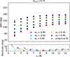 |
Fig. 3. Top: Mean ΔPA values (from a full period) for different models in our library, overlaid with our empirical fitting relation. Bottom: Residuals (percentage difference between ΔPA and δPA0 → 1), where for every radius the spin values have been expanded horizontally for clarity. |
In the following section we demonstrate its application through explicit examples.
4.4. Mock ΔPA observation
Equation (13) can be solved analytically for a*, but the resulting expression is cumbersome and impractical to present here. Instead, a more convenient approach is to substitute observed values and solve for a*. In our case, we employed a Bayesian solver using dynesty, a nested sampling tool introduced by Speagle (2020) and further developed by Koposov et al. (2023).
This choice for a Bayesian approach is motivated by two key advantages: (1) it provides a natural framework for incorporating observational uncertainties through Gaussian priors with specified standard deviations, and (2) it yields a posterior distribution for the spin parameter, inherently accounting for measurement uncertainties. By assuming a uniform prior on spin, a* ∈ ( − 1, 1), the resulting posterior directly reflects the inferred constraints on a*. For the likelihood calculation, we used
![Mathematical equation: $$ \begin{aligned} \mathcal{L} (\boldsymbol{p}) = -\frac{\left[\Delta PA-\hat{\Delta PA}(\boldsymbol{p})\right]^2}{2\sigma _{\Delta PA}^2}\,, \end{aligned} $$](/articles/aa/full_html/2026/03/aa55277-25/aa55277-25-eq16.gif) (15)
(15)
where p is the vector of the model parameters (P, rhs, a*), ΔPA is the observed value, while  is the predicted value from our empirical relation in Eq. (13). The uncertainty σΔPA is taken from observations.
Note that P and rhs are observed with their own uncertainties (σP, σrhs) but still resampled using their Gaussian distributions as prior (including the full parameter space). This is a similar approach to including all three observables in the ℒ function and only sampling a*, but better, because it extracts more information from the system, since the posteriors can have shifted peaks from the mean of the observation. It also provides a more intuitive framework, since it samples 3 values (rhs, P and a*) and extracts ΔPA that is then compared to the observation.
Given the simplicity of the task, we employed dynamic nested sampling with 1000 live points, one additional batch, and default walker and bound settings. The computation takes approximately one minute on a standard Jupyter notebook running on a typical laptop. The script for this analysis is publicly available at GitHub2.
We simulated observations in which two bright spots can be identified on the screen, corresponding to the primary and secondary images of a hot spot, while following the same assumptions as our analysis modeling. A test on a more general case of non-equatorial, spiraling hot spots, is beyond the scope of the current work. In terms of accuracy, the ring diameter was measured as  as in EHTC (2022a). Based on this, we assumed a comparable level of accuracy for rhs (±0.5, M) and ΔPA (±5°). Using these uncertainties, we constructed three models, which are summarized in Table 3. The errors of ΔPA are used for the likelihood calculation of Eq. (15), while the errors of the other two parameters are used to define the prior space as a Gaussian distributions.
Mock observation parameters, including the a* from our fits.
Before presenting the results, there is a subtle point from our empirical relation (Eq. (13)) that is worth clarifying. The way we modeled orbital velocity facilitates comparisons with numerical and analytical disk solutions; however, Ωcoef itself is not directly observable. Instead, observations provide measurements of P and rhs, which can be related to Ωcoef and a* through Eq. (8). This implies that we effectively have two equations with two unknowns.
To illustrate this, we present Fig. 4, where we use test 1 as a template of observation and perform two different estimations. In the left case, we estimate Ωcoef and a* using two different fits: the “ΔPA fit”, which relies on our empirical relation (Eq. (13)), and the “P fit”, which is based on Eq. (8). The “P fit” constrains Ωcoef but leaves a* completely unconstrained, whereas the “ΔPA fit” has no direct constraint on Ωcoef and only weakly excludes the most extreme spin values.
The bottom-middle panel on the left of Fig. 4 shows the two-dimensional posterior distribution of Ωcoef and a*. Although each individual fit allows a* to span nearly the full prior range, their overlap (highlighted by a black circle) demonstrates how combining the two distributions leads to a well-defined solution. This provides a clear validation of our method’s effectiveness.
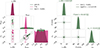 |
Fig. 4. Bayesian fit using the mock observations, the uncertainties from Table 3, and the empirical relation of Eq. (13). Left: Fits using Eqs. (13) and (8) (period) separately. Right: Fit when combining the two. |
Instead of using a two-step approach that involves overlapping fits of the two equations, we could incorporate the exploration of Ωcoef within a single algorithm, as shown on the right side of Fig. 4. In this case, Ωcoef is directly obtained from Eq. (14) and substituted into the empirical relation. Consequently, it is not treated as a free parameter in the prior and does not appear in the posteriors. Naturally, given the values of rhs, P, and a*, Ωcoef is fully determined. As expected from the previous exercise the spin parameter is nicely constrained at a* = −0.16 ± 0.32 with 2σ confidence.
The results from tests 2 and 3 are presented in Fig. 5. The overall behavior remains consistent with test 1, with one notable difference: the constraining power improves when the spin values are closer to the boundaries. This is evident in the case of  , where the uncertainties are less than half those of tests 1 and 3. This behavior is expected, as the true value lies near the boundaries, but it is worth highlighting.
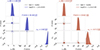 |
Fig. 5. Bayesian fit using the mock observations, the uncertainties from Table 3, and the empirical relation of Eq. (13). Note that only a* is the true constraint here; rhs and P are resampled for error propagation. |
5. Discussion and conclusions
The measurement of a black hole’s spin has occupied astrophysicists for decades, even before the first black hole image from the EHT Collaboration (EHTC 2019b). With upcoming upgrades to the EHT and next-generation EHT facilities, advancements in imaging algorithms, and the development of new projects such as BHEX, novel opportunities for spin estimation have emerged (and will continue to do so). This work explores one such avenue, leveraging the interpretation of flaring events around supermassive black holes, particularly Sgr A*, as emission from a well-localized region, a hot spot. This emission is expected to be sufficiently dominant, thus making the secondary image of the hot spot detectable and opening new possibilities for probing the near-horizon space-time. Among the potential observables, we identify the difference in position angle between the primary (n = 0) and secondary (n = 1) hot spot images (ΔPA) as a key diagnostic tool.
In this work we have presented three key results that facilitate the use of this observable, under the assumptions of circular and equatorial orbits:
-
We derived the correction to the complete elliptical integrals in the analytic relation for δPA, enabling the calculation of δPA0 → 1 with sub-degree accuracy, instead of the commonly used n → ∞ limit. Additionally, we propose a simplified approximation of the analytic solution that deviates by at most 5° at a* → 1 for the same δPA0 → 1 quantity.
-
We highlight a distinct effect of orbiting hot spots with regards to the system’s inclination angle (i). Specifically, when tracking the values of ΔPA over a full orbit of a moving hot spot, we find that the mean value of ΔPA remains unchanged (sub-degree for all cases apart from rhs = 4, a* = −0.9, where the deviation is 3° ) for inclinations up to i ∼ 30°, with deviation of ∼5° emerging at i ∼ 60°. This finding significantly simplifies our method, as otherwise, even at i ∼ 25° – the expected inclination for Sgr A* – the fluctuations of ΔPA would require a full curve analysis and thus a more complicated comparison with models.
-
After studying a large library of more than 900 models generated using the general relativistic radiative transfer code ipole, we achieved our primary goal: constructing a simple empirical relation for estimating spin based on ΔPA observations. This method matches the analytic solution to within 5° in most cases, with a maximum deviation of 10° for rhs ≤ 4 M. To further demonstrate the viability of this method, we conducted three tests, using mock observations with realistic uncertainties, and successfully extracted the spin in all cases, with a maximum uncertainty of ±0.3 for 2σ confidence. This is not a complete solution to the hot spot phenomenology, which can increase severely in modeling complexity, but rather a proof of concept for the usage of secondary images as space-time probes.
In the case of an observation that does not capture a full period but, for instance, 50% of it, we can still obtain valuable constraints with a more dedicated analysis. One approach is to assume an inclination angle (i ∼ 25°) and compare the ΔPA curve for several candidate values of the position angle (PA) of the black hole spin axis on the sky. This is necessary in order to model the correct phase of the curve. Independent estimates of PA include PA ∼ 130° (Ball et al. 2021; Yfantis et al. 2024a) and PA ∼ 180° (Wielgus et al. 2022b; GRAVITY Collaboration 2023; Yfantis et al. 2024b). From that we were able to extract the mean ΔPA and continue to use our method. A more robust method would be to create an adaptive Bayesian algorithm utilizing bipole, similarly to Yfantis et al. (2024a,b), and explore the full parameter space, jointly fitting for i, PA, rhs, Ωcoef, and a*. While this approach requires significantly more computational time (up to ten days, compared to one minute for the current method), it yields a comprehensive posterior over all relevant parameters.
Looking forward, further refinement of this method could focus on expanding the parameter space to include infalling or outgoing orbits; this expansion would more readily reproduce the equatorial motions seen in general relativistic magnetohydrodynamics. Another interesting addition would be the inclusion of non-equatorial orbits; these could address a big question pertaining to the tracking of flaring structures, regarding the mechanism for hot spot creation, with off-equatorial spots often related to plasmoids rather than flux tubes. Another interesting avenue would be the creation of a machine learning algorithm that uses an expanded library that treats hot spot observational data more generally, including potentially partial sampling the time-dependent astrometry for both images (n = 0, 1) and extracting all the information for the system (i, rhs, Ωcoef, radial velocities, etc.).
Acknowledgments
We thank the anonymous EHT internal reviewer for their comments. This publication is a part of the project Dutch Black Hole Consortium (with project number NWA 1292.19.202) of the research program of the National Science Agenda which is financed by the Dutch Research Council (NWO).
References
- Aimar, N., Dmytriiev, A., Vincent, F. H., et al. 2023, A&A, 672, A62 [NASA ADS] [CrossRef] [EDP Sciences] [Google Scholar]
- Antonopoulou, E., & Nathanail, A. 2024, A&A, 690, A240 [NASA ADS] [CrossRef] [EDP Sciences] [Google Scholar]
- Ball, D., Özel, F., Christian, P., Chan, C.-K., & Psaltis, D. 2021, ApJ, 917, 8 [NASA ADS] [CrossRef] [Google Scholar]
- Bardeen, J. M., Press, W. H., & Teukolsky, S. A. 1972, ApJ, 178, 347 [Google Scholar]
- Beckwith, K., & Done, C. 2005, MNRAS, 359, 1217 [NASA ADS] [CrossRef] [Google Scholar]
- Begelman, M. C., Scepi, N., & Dexter, J. 2022, MNRAS, 511, 2040 [NASA ADS] [CrossRef] [Google Scholar]
- Broderick, A. E., & Loeb, A. 2006, MNRAS, 367, 905 [Google Scholar]
- Claudel, C.-M., Virbhadra, K. S., & Ellis, G. F. R. 2001, J. Math. Phys., 42, 818 [Google Scholar]
- Conroy, N. S., Bauböck, M., Dhruv, V., et al. 2023, ApJ, 951, 46 [CrossRef] [Google Scholar]
- Dexter, J., Tchekhovskoy, A., Jiménez-Rosales, A., et al. 2020, MNRAS, 497, 4999 [Google Scholar]
- Doeleman, S. S., Barrett, J., Blackburn, L., et al. 2023, Galaxies, 11, 107 [NASA ADS] [CrossRef] [Google Scholar]
- EHTC (Akiyama, K., et al.) 2019a, ApJ, 875, L5 [Google Scholar]
- EHTC (Akiyama, K., et al.) 2019b, ApJ, 875, L1 [Google Scholar]
- EHTC (Akiyama, K., et al.) 2022a, ApJ, 930, L15 [NASA ADS] [CrossRef] [Google Scholar]
- EHTC (Akiyama, K., et al.) 2022b, ApJ, 930, L12 [NASA ADS] [CrossRef] [Google Scholar]
- EHTC (Akiyama, K., et al.) 2022c, ApJ, 930, L13 [NASA ADS] [CrossRef] [Google Scholar]
- EHTC (Akiyama, K., et al.) 2022d, ApJ, 930, L16 [NASA ADS] [CrossRef] [Google Scholar]
- EHTC (Akiyama, K., et al.) 2024a, A&A, 681, A79 [NASA ADS] [CrossRef] [EDP Sciences] [Google Scholar]
- EHTC (Akiyama, K., et al.) 2024b, ApJ, 964, L26 [CrossRef] [Google Scholar]
- Galison, P., Johnson, M. D., Lupsasca, A., Gravely, T., & Berens, R. 2024, in Space Telescopes and Instrumentation 2024: Optical, Infrared, and Millimeter Wave, eds. L. E. Coyle, S. Matsuura, & M. D. Perrin, Int. Soc. Opt. Photonics (SPIE), 13092, 130926R [Google Scholar]
- Gelles, Z., Himwich, E., Johnson, M. D., & Palumbo, D. C. M. 2021, Phys. Rev. D, 104, 044060 [NASA ADS] [CrossRef] [Google Scholar]
- Gralla, S. E., & Lupsasca, A. 2020, Phys. Rev. D, 101, 044031 [NASA ADS] [CrossRef] [Google Scholar]
- Gralla, S. E., Holz, D. E., & Wald, R. M. 2019, Phys. Rev. D, 100, 024018 [Google Scholar]
- Gralla, S. E., Lupsasca, A., & Marrone, D. P. 2020, Phys. Rev. D, 102, 124004 [NASA ADS] [CrossRef] [Google Scholar]
- GRAVITY Collaboration (Abuter, R., et al.) 2018, A&A, 618, L10 [NASA ADS] [CrossRef] [EDP Sciences] [Google Scholar]
- GRAVITY Collaboration (Abuter, R., et al.) 2020a, A&A, 638, A2 [NASA ADS] [CrossRef] [EDP Sciences] [Google Scholar]
- GRAVITY Collaboration (Bauböck, M., et al.) 2020b, A&A, 635, A143 [CrossRef] [EDP Sciences] [Google Scholar]
- GRAVITY Collaboration (Jiménez-Rosales, A., et al.) 2020c, A&A, 643, A56 [CrossRef] [EDP Sciences] [Google Scholar]
- GRAVITY Collaboration (Abuter, R., et al.) 2022, A&A, 657, L12 [NASA ADS] [CrossRef] [Google Scholar]
- GRAVITY Collaboration (Abuter, R., et al.) 2023, A&A, 677, L10 [NASA ADS] [CrossRef] [EDP Sciences] [Google Scholar]
- Haggard, D., Nynka, M., Mon, B., et al. 2019, ApJ, 886, 96 [NASA ADS] [CrossRef] [Google Scholar]
- Hamaus, N., Paumard, T., Müller, T., et al. 2009, ApJ, 692, 902 [NASA ADS] [CrossRef] [Google Scholar]
- Johannsen, T., & Psaltis, D. 2010, ApJ, 718, 446 [NASA ADS] [CrossRef] [Google Scholar]
- Johnson, M. D., Lupsasca, A., Strominger, A., et al. 2020, Sci. Adv., 6, eaaz1310 [NASA ADS] [CrossRef] [Google Scholar]
- Johnson, M. D., Akiyama, K., Baturin, R., et al. 2024, in Space Telescopes and Instrumentation 2024: Optical, Infrared, and Millimeter Wave, eds. L. E. Coyle, S. Matsuura, & M. D. Perrin, SPIE Conf. Ser., 13092, 130922D [Google Scholar]
- Kocherlakota, P., Rezzolla, L., Roy, R., & Wielgus, M. 2024, MNRAS, 531, 3606 [NASA ADS] [CrossRef] [Google Scholar]
- Koposov, S., Speagle, J., Barbary, K., et al. 2023, Zenodo [Google Scholar]
- Levis, A., Chael, A. A., Bouman, K. L., Wielgus, M., & Srinivasan, P. P. 2024, Nat. Astron., 8, 765 [NASA ADS] [CrossRef] [Google Scholar]
- Lupsasca, A., Cárdenas-Avendaño, A., Palumbo, D. C. M., et al. 2024, in Space Telescopes and Instrumentation 2024: Optical, Infrared, and Millimeter Wave, eds. L. E. Coyle, S. Matsuura, & M. D. Perrin, SPIE Conf. Ser., 13092, 130926Q [Google Scholar]
- Mościbrodzka, M., & Gammie, C. F. 2018, MNRAS, 475, 43 [CrossRef] [Google Scholar]
- Najafi-Ziyazi, M., Davelaar, J., Mizuno, Y., & Porth, O. 2024, MNRAS, 531, 3961 [NASA ADS] [CrossRef] [Google Scholar]
- Narayan, R., Igumenshchev, I. V., & Abramowicz, M. A. 2003, PASJ, 55, L69 [NASA ADS] [Google Scholar]
- Porth, O., Mizuno, Y., Younsi, Z., & Fromm, C. M. 2021, MNRAS, 502, 2023 [NASA ADS] [CrossRef] [Google Scholar]
- Ripperda, B., Bacchini, F., & Philippov, A. A. 2020, ApJ, 900, 100 [NASA ADS] [CrossRef] [Google Scholar]
- Ripperda, B., Liska, M., Chatterjee, K., et al. 2022, ApJ, 924, L32 [NASA ADS] [CrossRef] [Google Scholar]
- Scepi, N., Dexter, J., & Begelman, M. C. 2022, MNRAS, 511, 3536 [NASA ADS] [CrossRef] [Google Scholar]
- Speagle, J. S. 2020, MNRAS, 493, 3132 [Google Scholar]
- Tiede, P., Pu, H.-Y., Broderick, A. E., et al. 2020, ApJ, 892, 132 [NASA ADS] [CrossRef] [Google Scholar]
- Trippe, S., Paumard, T., Ott, T., et al. 2007, MNRAS, 375, 764 [NASA ADS] [CrossRef] [Google Scholar]
- Vincent, F. H., Wielgus, M., Aimar, N., Paumard, T., & Perrin, G. 2024, A&A, 684, A194 [NASA ADS] [CrossRef] [EDP Sciences] [Google Scholar]
- Vos, J., Mościbrodzka, M. A., & Wielgus, M. 2022, A&A, 668, A185 [NASA ADS] [CrossRef] [EDP Sciences] [Google Scholar]
- Vos, J. T., Olivares, H., Cerutti, B., & Mościbrodzka, M. 2024, MNRAS, 531, 1554 [NASA ADS] [CrossRef] [Google Scholar]
- Walia, R. K., Kocherlakota, P., Chang, D. O., & Salehi, K. 2025, Phys. Rev. D, 111, 104074 [Google Scholar]
- Wielgus, M., Marchili, N., Martí-Vidal, I., et al. 2022a, ApJ, 930, L19 [NASA ADS] [CrossRef] [Google Scholar]
- Wielgus, M., Moscibrodzka, M., Vos, J., et al. 2022b, A&A, 665, L6 [NASA ADS] [CrossRef] [EDP Sciences] [Google Scholar]
- Wong, G. N. 2021, ApJ, 909, 217 [NASA ADS] [CrossRef] [Google Scholar]
- Yfantis, A., Wielgus, M., & Moscibrodzka, M. 2024a, A&A, 691, A327 [NASA ADS] [CrossRef] [EDP Sciences] [Google Scholar]
- Yfantis, A. I., Mościbrodzka, M. A., Wielgus, M., Vos, J. T., & Jimenez-Rosales, A. 2024b, A&A, 685, A142 [NASA ADS] [CrossRef] [EDP Sciences] [Google Scholar]
- Zhang, Z., Hou, Y., Guo, M., Mizuno, Y., & Chen, B. 2025, Phys. Rev. D, 112, 083024 [Google Scholar]
- Zhou, L., Zhong, Z., Chen, Y., & Cardoso, V. 2025, Phys. Rev. D, 111, 064075 [Google Scholar]
Note that ray-tracing of general relativistic magnetohydrodynamic snapshots is typically done in fast light (EHTC 2019a, 2022d).
Appendix A: Numerical inspections
In this section we provide proof from two important tests of the simulation procedure. The first test regards the orbital velocities of the first and second images, and in particular whether the observed speeds correspond to the input on the simulation domain. The results are visible in Fig. A.2, where we show the phase of the two images, extracted from the centroid of every spot in the image domain, using the regular setup of 256x256 pixels. It is clear that the velocities in the image domain exactly follow the theoretical value, which holds even in the case of a high inclination i = 60°, where the speed changes in different parts of the orbit due to the viewing angle, but overall from start to finish the velocity is the same.
The second test, visible in Fig. A.1 is the convergence of higher order images (referring to n = 2 here) to the theoretical expectation of δPA. Additionally, it serves excellently as a demonstration of the dimness of n = 2, where the fluxes for the three spots are I0 = 0.705, I1 = 0.050, I2 = 0.003, meaning it is virtually impossible to expect n = 2 to interfere with any observations in the near to mid future.
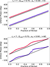 |
Fig. A.1. Orbital phase for two models with the same parameters apart from inclination: i = 0 (top) and i = 60° (bottom). The phase has been calculated using the centroids in the image domain. The black line with "x" points is the theoretical velocity used in the simulation. |
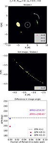 |
Fig. A.2. Top: Snapshot from a non-moving hot spot, using a higher resolution of 1024x1024 pixels, to resolve the third image. Middle: Zoomed-in view of the third image. Bottom: ΔPA n(0 − 1) measurement from the first to the second image, and ΔPA n(1 − 2) from the second to the third. The dash-point line denotes the theoretical expectation δPA(n → ∞). |
All Tables
All Figures
|
Fig. 1. Left: Snapshot from a hot spot movie, with resolution 256 × 256 (as in the entire library), where ΔPA is calculated from the primary to the secondary counterclockwise. Middle: Curve of ΔPA measurement with respect to time for a full period. Right: Time lag (difference in arrival times) between the first and second image. The gray vertical line in the right panels denotes the snapshot’s time in the left panels. |
| In the text | |
|
Fig. 2. Distribution (violins) of ΔPA values during a full period for different inclination values. The crosses denote the average values per period and the dashed lines the value at i = 0° for a fixed a*. |
| In the text | |
|
Fig. 3. Top: Mean ΔPA values (from a full period) for different models in our library, overlaid with our empirical fitting relation. Bottom: Residuals (percentage difference between ΔPA and δPA0 → 1), where for every radius the spin values have been expanded horizontally for clarity. |
| In the text | |
|
Fig. 4. Bayesian fit using the mock observations, the uncertainties from Table 3, and the empirical relation of Eq. (13). Left: Fits using Eqs. (13) and (8) (period) separately. Right: Fit when combining the two. |
| In the text | |
|
Fig. 5. Bayesian fit using the mock observations, the uncertainties from Table 3, and the empirical relation of Eq. (13). Note that only a* is the true constraint here; rhs and P are resampled for error propagation. |
| In the text | |
|
Fig. A.1. Orbital phase for two models with the same parameters apart from inclination: i = 0 (top) and i = 60° (bottom). The phase has been calculated using the centroids in the image domain. The black line with "x" points is the theoretical velocity used in the simulation. |
| In the text | |
|
Fig. A.2. Top: Snapshot from a non-moving hot spot, using a higher resolution of 1024x1024 pixels, to resolve the third image. Middle: Zoomed-in view of the third image. Bottom: ΔPA n(0 − 1) measurement from the first to the second image, and ΔPA n(1 − 2) from the second to the third. The dash-point line denotes the theoretical expectation δPA(n → ∞). |
| In the text | |
Current usage metrics show cumulative count of Article Views (full-text article views including HTML views, PDF and ePub downloads, according to the available data) and Abstracts Views on Vision4Press platform.
Data correspond to usage on the plateform after 2015. The current usage metrics is available 48-96 hours after online publication and is updated daily on week days.
Initial download of the metrics may take a while.