| Issue |
A&A
Volume 707, March 2026
|
|
|---|---|---|
| Article Number | A30 | |
| Number of page(s) | 16 | |
| Section | Catalogs and data | |
| DOI | https://doi.org/10.1051/0004-6361/202555435 | |
| Published online | 02 March 2026 | |
Search for quasar pairs with Gaia astrometric data
I. Method and candidates
1
School of Physics and Astronomy, Beijing Normal University,
Beijing
100875
China
2
Institute for Frontier in Astronomy and Astrophysics, Beijing Normal University,
Beijing
102206
China
3
College of Intelligent Systems Science and Engineering, Hubei Minzu University,
Enshi,
Hubei
445000
China
4
Department of Physics, Nanchang University,
Nanchang
330031
China
5
Center for Relativistic Astrophysics and High Energy Physics, Nanchang University,
Nanchang
330031
China
6
Purple Mountain Observatory, Chinese Academy of Sciences,
Nanjing,
Jiangsu
210023
China
★ Corresponding author: This email address is being protected from spambots. You need JavaScript enabled to view it.
Received:
8
May
2025
Accepted:
8
January
2026
Abstract
Quasar pairs, a special subclass of galaxy pairs, are valuable in the investigation of quasar interaction and clustering, the coevolution between the two quasars’ host galaxies, and the growth of supermassive black holes, as well as the formation and evolution of galaxies overall. However, quasar pairs on kiloparsec scales are observationally rare. The scarcity of available samples hindered the deeper exploration and statistics of these objects. In this work, we apply an astrometric method to systematically search for quasar candidates within a transverse distance of 100 kpc to known quasars in the Million Quasar Catalog. These candidates are Gaia sources with proper motions and parallaxes that are consistent with zero. A visual inspection of the sample was performed to remove the contamination of crowded stellar fields and nearby galaxies. A total of 4112 quasar pair candidates were isolated, with a median member separation of 8.81″, a median Gaia G-band magnitude of 20.52, and a median redshift of 1.61. Following a comparison of our catalog with three major candidate quasar pair catalogs, we identified 3984 new quasar pair candidates that had previously been overlooked in the three catalogs. Several interesting quasar pair candidates are highlighted and discussed in this work. We also offer a brief discussion of our quasar selection and several techniques for improving the success rate of quasar pair selection. Extensive spectroscopic follow-up campaigns are currently underway to validate their astrophysical nature.
Key words: methods: data analysis / methods: statistical / catalogs / astrometry / quasars: general
© The Authors 2026
 Open Access article, published by EDP Sciences, under the terms of the Creative Commons Attribution License (https://creativecommons.org/licenses/by/4.0), which permits unrestricted use, distribution, and reproduction in any medium, provided the original work is properly cited.
This article is published in open access under the Subscribe to Open model. This email address is being protected from spambots. You need JavaScript enabled to view it. to support open access publication.
1 Introduction
Quasars are a class of extremely luminous active galactic nuclei (AGNs), each hosting a supermassive black hole (SMBH) surrounded by an accretion disk from which powerful radiation originates. In the unified model of AGN, an extensive dusty torus surrounds the central engine and the broad-line regions (BLRs), with the BLRs situated on both sides of the accretion disk. The narrow-line regions (NLRs) extend beyond the torus, enveloping it at larger radial distances (e.g., Antonucci 1993; Urry & Padovani 1995; Netzer 2015). Since the discovery of quasars in the early 1960s (Schmidt 1963; Sandage 1965), numerous surveys have discovered close to a million objects of this kind (the Million Quasar Catalog, Flesch 2023). The most recently released DESI DR1 even reported 1.65 million quasars, substantially extending the known quasar population (DESI Collaboration 2025).
If two quasars or galaxies encounter and interact, they may form a type of system known as “quasar pair,” which makes up only a minute fraction of the general quasar population. Observationally, quasar pairs exhibit typical separations of less than several arcseconds and nearly identical redshifts, corresponding to sub-milliparsec (sub-Mpc) transverse physical distances. According to De Rosa et al. (2019), quasar pairs can be classified into two subclasses, dual quasar and binary quasar, based on the transverse distances between pair members. The dual quasar is defined as an interacting galaxy system containing two active nuclei that are not mutually gravitationally bound. The transverse distance between the two quasars ranges from ~1 pc to ~100 kpc. The binary quasar refers to two quasars that are gravitationally bound and forming a Keplerian binary. The two quasars are separated by a parsec (pc) to sub-pc transverse distance. Quasar pairs are natural results of the hierarchical evolution of galaxies. They are important laboratories to study the quasar interaction, coevolution between the two hosts, environment overdensity, clustering, large-scale structure, the growth of SMBHs, and the formation and evolution of galaxies in extreme environments as well as the early Universe (e.g., Begelman et al. 1980; Impey 1998; Yu 2002; Hennawi et al. 2006; Myers et al. 2008; Liu et al. 2011; Shen et al. 2010, 2023b; Merritt 2013; Sandrinelli et al. 2014; Sandrinelli et al. 2018; Richarte et al. 2025; Hou et al. 2020; An et al. 2022; Xu et al. 2024; Wang et al. 2023b). They are also potential origins of nanohertz gravitational waves (nHz-GWs) in the early Universe (Kelley et al. 2019; Chen et al. 2020; Shen et al. 2023a).
However, the rarity of confirmed quasar pairs inhibited deep exploration and statistical investigations. According to recent statistical work, only ~ 160 quasar pairs with a transverse distance of less than 100 kpc are publicly confirmed to date (Big MAC DR1, Pfeifle et al. 2025). It is therefore important to search for more of them. The search for quasar pairs can be dated back to Stockton (1972) and Wampler et al. (1973). However, their discoveries are not true quasar pairs but projected cases. The first populations of quasar pairs were discovered by some optical and radio surveys (e.g., Bolton et al. 1976; Meylan et al. 1987; Djorgovski et al. 1987; Muñoz et al. 1998). With the successive launches of large-scale imaging sky surveys such as SDSS (York et al. 2000), WISE (Wright et al. 2010), Pan-STARRS (Chambers et al. 2016), and recent DESI Legacy Imaging Surveys (DESI-LS, Dey et al. 2019), a significant number of quasar pairs and their candidates have been discovered by utilizing a color-based method and spectroscopic follow-up (e.g., Hennawi et al. 2010; Green et al. 2010; Chen 2021). Several tens of quasar pairs have also been discovered as by-products of the search for strongly lensed quasars (e.g., Yue et al. 2023; Dawes et al. 2023; He et al. 2025), for example, the Binary Quasar sub-catalog compiled from the Gravitationally lensed quasars in Gaia project1 (GLQG, Lemon et al. 2017). Furthermore, a recently proposed image decomposition method has also discovered a few quasar pairs (e.g., Silverman et al. 2020; Tang et al. 2021). Combining optical imaging and spectroscopic surveys seems to be a promising and efficient approach to searching for quasar pairs.
In addition, several indirect methods have been used to search for quasar pairs with various characteristics, such as periodic variability (Sillanpää et al. 1988; Graham et al. 2015b,a; Liao et al. 2021; Davis et al. 2024), radial velocity drift (Guo et al. 2019; Zheng et al. 2023), double-peaked emission lines (Zhou et al. 2004; Boroson & Lauer 2009; Tang & Grindlay 2009; Shen & Loeb 2010; Kim et al. 2020a,b; Zheng et al. 2024), asymmetric emission line profiles (Eracleous et al. 2012a), and continuum anomalies (Yan et al. 2015), as well as the observations of binary active cores in radio or X-ray images (Liu et al. 2003; Komossa et al. 2003). However, these indirect methods are not entirely reliable. The periodic variability induced by orbital motion can be easily imitated by the intrinsic irregular variability of the quasars (Charisi et al. 2016). Accretion disks can also produce double-peaked emission line profiles (Eracleous et al. 1997, 2012b), and some double-peaked narrow-line objects have been confirmed to be single sources (Foord et al. 2020). A single source can also produce velocity drift and a double-peaked profile, while altering the profile of emission lines (Du & Wang 2023). Methods based on color or the spectral energy distribution (SED) also have their limitations, as the quasar region in the color-color diagram is heavily contaminated by some specific spectral types of stars (Ross et al. 2012; Wu et al. 2012; Yèche et al. 2020).
The astrometric search for quasars is one of the most remarkable and promising methods. Quasars are observed as nearly stationary objects on the celestial sphere due to their enormous distance from Earth. Quasar selection with the astrometric method can be traced back to Koo et al. (1986). They separated quasars from white dwarfs with the assistance of a proper motion criterion and demonstrated the power of the astrometric method. To make efficient and unbiased searches for quasars, several efforts have drawn on the astrometric method (e.g., Shu et al. 2019; Wu et al. 2023). For instance, Heintz et al. (2015, 2018, 2020) applied a pure astrometric method to select quasars and derived a conservative selection efficiency of ~75%, indicating great success in quasar selection with astrometry. Lemon et al. (2019) presented a stricter criterion of proper motion significance (PMSIG) to assist the search for lensed quasars. Similarly, a probability-based zero-proper motion method (fPM0), which is more complete in a computational sense than PMSIG, was proposed to help select quasar candidates behind the Galactic plane (GPQ, Fu et al. 2021). The probability-based zero-proper motion method was also used in Fu et al. (2024) and Fu et al. (2025) to construct a whole sky candidate quasar catalog. These efforts validate the capability of astrometry in quasar selection.
For the quasar pair search, the joint significance of the total proper motion χ2 successfully selected some quasar pairs with quite small member separations around 1″ (Souchay et al. 2022; Makarov & Secrest 2022). On the other hand, some novel methods have also discovered several tens of spatially unresolved or marginally resolved dual AGNs, quasars, and SMBHs that are separated by less than 1″ (from sub-kpc to a few kpc). These discoveries open up new avenues to in-depth exploration of the “final parsec” problem, which refers to the theoretical difficulty of bringing two SMBHs from a parsec-scale separation to a distance where gravitational wave emission can efficiently drive them to final coalescence (e.g., Milosavljević & Merritt 2001; Merritt & Milosavljević 2005; Zhang 2023; Bromley et al. 2024; Koo et al. 2024). These novel methods include anomalous astrometry (Makarov et al. 2012; Makarov & Secrest 2023; Wu et al. 2022; Ji et al. 2023), optical flickering or photometric centroid shift (e.g., Liu 2015, 2016), Gaia multipeak (GMP, Mannucci et al. 2022, 2023; Ciurlo et al. 2023; Scialpi et al. 2024; Wu et al. 2024), and astrometric jitter and disturbance techniques (Vastrometry, Shen et al. 2019, 2021; Uppal et al. 2024; Hwang et al. 2020). Vastrometry was initially used in an optical-band project titled Vastrometry for Off-nucleus and Dual sub-Kpc AGN (VODKA, e.g., Chen et al. 2022, 2023b, 2025) and has recently been applied to radio bands within the framework of Varstrometry for Dual AGN using Radio interferometry (VaDAR, e.g., Wang et al. 2023a; Schwartzman et al. 2024). In contrast to the aforementioned small-separation pairs, a serendipitously discovered quasar pair at z = 1.76 and with a member separation of 8.76″ indicates that the selection of point sources without significant proper motion next to known quasars could be an effective way to search for quasar pairs across a wider range of member separations (Altamura et al. 2020).
Referring to the probability-based astrometric criteria from Fu et al. (2021) and inspired by Altamura et al. (2020), we initiated a systematic search for new quasars located in the vicinity of known quasars to find new quasar pairs with a combination of Gaia astrometric data and the Million Quasar Catalog (MQC). This paper details that search and is organized as follows. The data exploited in this work, method details, and the derived candidates are introduced in Section 2. The basic statistical and color properties of the quasar pair candidates, the comparative advantages of our sample over three major candidate quasar pair catalogs, and several interesting candidates are described in Section 3. The discussion on our selection and future improvement is given in Section 4. We summarise our conclusions in Section 5. Throughout this paper, we adopt a flat lambda cold dark matter (λCDM) cosmology with Ωλ = 0.7, ΩM = 0.3, and H0 = 70 km s−1 Mpc−1.
2 Data and method
The catalogs used in this work include version 8.0 of MQC and Gaia Data Release 3 (Gaia DR3). The imaging data of DESI-LS and Pan-STARRS were used to visually inspect and refine the astrometrically selected quasar pair candidates.
2.1 Data
The MQC builds on the Half Million Quasar Catalog (Flesch 2015). The sources included in this catalog can be traced back to the first release (version 0.1) on April 22, 2009. After 14 years of continuous expansion and the addition of quasar samples confirmed from large numbers of multiband photometric and spectroscopic surveys, the final version 8.0 of the MQC (hereafter, MQCv8)2 was published on August 2, 2023 (Flesch 2023). The MQCv8 contains 1 021 800 quasars and high-probability candidates, 60.7% of which possess Gaia DR3 astrometry. As the SDSS DR16Q (Lyke et al. 2020) constitutes the primary source of this catalog, the resulting large and robust quasar sample provides a sufficient basis for a systematic search for quasar pairs.
Gaia is a powerful space astrometric satellite launched by the European Space Agency (ESA) in December 2013. The mission is for a space-based, astrometric, and photometric all-sky survey at optical wavelengths, providing more than one billion accurate measurements of astrometric parameters for a variety of objects (de Bruijne 2012; Gaia Collaboration 2016). Under the Gaia’s unprecedented measurement accuracy of a few microarcseconds, extragalactic sources and objects in the Milky Way can be distinguished effectively by astrometric parameters such as proper motion and parallax. Gaia published its DR3 on June 13, 2022 (Gaia Collaboration 2023), containing 1.8 billion astrometric objects and 1.5 billion sources with measured proper motions and parallaxes, with an accuracy as high as 0.001 mas/yr.
2.2 Method
Based on the combination of the latest MQC and the most enormous astrometric database, searching for extragalactic sources with proper motion and parallax results consistent with zero near the spectroscopically confirmed quasars has immense advantages in the catalog volume, astrometric accuracy, and the quasar selection bias. The following three major steps are executed to obtain the quasar pair candidates:
- (1)
cross-match between MQCv8 and Gaia DR3;
- (2)
astrometric filtering on the cross-matched catalog;
- (3)
visual inspection of the astrometrically selected pair candidates.
2.2.1 Cross-match
The catalog cross-matching tool TOPCAT (Taylor 2005) was employed to carry out the first step of our method. To start with, quasars in MQCv8 were searched for in the SIMBAD database3 (Wenger et al. 2000) using a 1″ radius to update their redshift. To search for higher-redshift quasar pair candidates and extend the existing quasar pair catalog, quasars with z > 0.5 were selected as the base sample, which includes 908 990 quasars. We then crossmatched this quasar base sample with Gaia DR3 using a search radius of 1″ to exclude quasars with imprecise radio or X-band positions. The Gaia match closest to the position of the quasar was considered as its Gaia counterpart. This yields a Gaia optical quasar sample, which consists of 582 725 quasars with Gaia detections.
Based on the updated redshift, the angular separation corresponding to a transverse distance of 100 kpc (angular diameter distance) to each optical quasar was calculated under the flat λCDM cosmology. These separations were used to perform the cross-match of Gaia DR3 sources to the optical quasars with Gaia positions. A total of 105 971 Gaia sources within 100 kpc to the MQCv8 quasars were selected to constitute a preliminary catalog, marked as 100kpcCAT. Then, the 100kpcCAT was searched again in SIMBAD within a radius of 1″ to exclude those spectroscopically confirmed sources. In addition, a magnitude cut of G ⩽ 21 mag was performed to ensure the reliability of the astrometric measurements (Gaia Collaboration 2023). Finally, a sample of 85 839 sources with proper motion and parallax measurements but without redshift was isolated as the input sample of the next step of the astrometric filtering. For convenience, we named this sample astrometricCAT.
2.2.2 Astrometric filtering
To support the astrometric filtering, reference samples of spectroscopically confirmed quasars and stars are required. SDSS, LAMOST, and DESI provide extensive spectral libraries of quasars and stars, making them ideal for reference sample construction. We retrieved all quasars and stars from SDSS DR18 (Almeida et al. 2023) via its Science Archive Server4 (SAS). For LAMOST, quasars and stars were extracted from its DR12 v1.0 general catalog5 (Cui et al. 2012). For DESI, quasars and stars were obtained from its recent DR16. All the sources were crossmatched with Gaia DR3 to extract sources that have both proper motion and parallax measurements.
Given the distinct Galactic coordinate distributions of quasars and stars, we randomly selected Gaia cross-matched quasars and stars within each of six Galactic latitude bins: 0° ⩽ |b| < 20°, 20° ⩽ |b| < 30°, 30° ⩽ |b| < 45°, 45° ⩽ |b| < 60°, 60° ⩽ |b| < 75°, and 75° ⩽ |b| ⩽ 90°. Each sky region bin contains equal numbers of quasars and stars. The selection generated a reference sample based on the sky region, which contains 704 942 quasars and the same number of stars. It is denoted as Good_Sky for convenience and the quasar and star subsamples are denoted as GoodQSO_Sky and GoodSTAR_Sky, respectively.
Considering that the astrometric accuracy in Gaia DR3 is strongly dependent on source brightness (Gaia Collaboration 2023), another reference sample that is related to the Gaia G-band magnitude is required. To exclude extremely faint sources that may have poor astrometric accuracy and to ensure consistency with the range of the astrometricCAT’s Gaia G-band magnitude, we randomly sampled Gaia cross-matched quasars and stars according to three Gaia G-band magnitude bins: 12 ⩽ G < 19, 19 ⩽ G < 20, and 20 ⩽ G ⩽ 21. Each magnitude bin contains equal numbers of quasars and stars. Moreover, the random sampling was designed to ensure identical G-band magnitude distributions between quasars and stars. This design can eliminate the impact of magnitude discrepancy on astrometric filtering. The sampling generated a reference sample based on the magnitude, which contains 697 779 quasars and the same number of stars. Similarly, it is denoted as Good_Mag and the quasar and star subsamples are denoted as GoodQSO_Mag and GoodSTAR_Mag, respectively.
The distributions of the Good_Sky and Good_Mag in equatorial coordinates are displayed in Figure 1. The equal volume of the sky region binned or magnitude binned quasar and star subsamples ensures an unbiased astrometric filtering. The two reference samples are the keys to the astrometric filtering.
Utilizing several astrometric measurements provided by Gaia DR3, two types of astrometric criteria are proposed to select extragalactic candidates efficiently. The astrometric measurements include the proper motion in right ascension and declination (pmRA and pmDE), proper-motion uncertainties in the two directions (e_pmRA and e_pmDE), the correlation coefficient between pmRA and pmDE (pmRApmDEcor), parallax (Plx), and parallax uncertainties (e_Plx). Following Fu et al. (2021), the probability density of zero proper motion is employed to set the astrometric criteria. Equation (10) in Fu et al. (2021) defines the probability density of zero proper motion of a Gaia DR2 source, but several of its parameters are no longer applicable to Gaia DR3. Therefore, we adopted Equation (7) in Fu et al. (2024) to calculate the probability density of zero proper motion of a Gaia DR3 source,
![Mathematical equation: $\matrix{{{f_{0pm}} = } \hfill & {{1 \over {2\pi {\sigma _{{\mu _{{\alpha ^ * }}}}}{\sigma _{{\mu _\delta }}}\sqrt {1 - \rho } }}} \hfill \cr {} \hfill & { \times exp\left\{ { - {1 \over {2\left( {1 - {\rho ^2}} \right)}}\left[ {{{\left( {{{{\mu _{{\alpha ^ * }}}} \over {{\sigma _{{\mu _{{\alpha ^ * }}}}}}}} \right)}^2} - {{2\rho {\mu _{{\alpha ^ * }}}{\mu _\delta }} \over {{\sigma _{{\mu _{{\alpha ^ * }}}}}{\sigma _{{\mu _\delta }}}}} + {{\left( {{{{\mu _\delta }} \over {{\sigma _{{\mu _\delta }}}}}} \right)}^2}} \right]} \right\},} \hfill \cr }$](/articles/aa/full_html/2026/03/aa55435-25/aa55435-25-eq1.png) (1)
where μα* is proper motion in right ascension, μδ is proper motion in declination, ρ is the correlation coefficient between μα* and μδ, and σμα*, and σμδ are the proper-motion uncertainties. According to the equation, sources with smaller proper motions will have larger f0pm under the same uncertainty level.
(1)
where μα* is proper motion in right ascension, μδ is proper motion in declination, ρ is the correlation coefficient between μα* and μδ, and σμα*, and σμδ are the proper-motion uncertainties. According to the equation, sources with smaller proper motions will have larger f0pm under the same uncertainty level.
Considering that the parallax of the nearby Galactic stars is generally significant, whereas extragalactic sources exhibit almost zero parallaxes, an additional criterion is introduced, namely, the probability density of zero parallaxes, to eliminate the Galactic stars with coincidental near-zero proper motion. Similarly, the probability density of zero parallax of a Gaia DR3 source is defined as
![Mathematical equation: ${f_{0plx}} = {1 \over {\sqrt {2\pi } {\sigma _\varpi }}} \cdot exp\left[ { - {1 \over 2} \cdot {{\left( {{\varpi \over {{\sigma _\varpi }}}} \right)}^2}} \right],$](/articles/aa/full_html/2026/03/aa55435-25/aa55435-25-eq2.png) (2)
where
(2)
where  and
and  are the parallax and its uncertainty, respectively. According to the definition, sources with smaller parallaxes will have larger f0plx under the same uncertainty level.
The f0pm and f0plx values were calculated for all sources in the Good_Sky, Good_Mag, and astrometricCAT. The logarithm of them (log f0pm and log f0plx) were adopted for better visualization. Figure 2 displays the log f0pm versus log f0plx distributions of the unbinned Good_Sky (left panel) and Good_Mag (right panel). Both distributions employ optimally determined thresholds of criteria through iterative attempts; specifically, log f0pm ⩾ −3 and log f0plx ⩾ −2. From the distribution of the sky region unbinned Good_Sky, it appears that this set of criteria effectively filters out the majority of stars. In contrast, the distribution of the magnitude unbinned Good_Mag indicates that a significant number of stars still cannot be efficiently removed.
To further examine whether the quasar selection efficiency is affected by sky region, the distributions of aforementioned six sky binned Good_Sky are plotted in Figure 3, along with the optimal thresholds of criteria, which were iteratively determined. Table 1 lists the quasar selection completeness, purity, and stellar contamination for each sky bin under the corresponding astrometric criteria. It is evident that when |b| ⩾ 20°, the completeness, purity, and stellar contamination of quasar selection remain stable at approximately 98%, 95%, and 5%, respectively, with increasing Galactic latitude. The determined thresholds of the criteria are identical in each sky bin, indicating that the quasar selection efficiency is almost unaffected by sky region, at least within the context of this work. This result markedly differs from the conclusions of Heintz et al. (2020, hereafter, Heintz20), where quasar selection purity increases from ~20% to ~80% with increasing Galactic latitude. The underlying reasons are explained and discussed in Section 4.1.
In the 0° ⩽ |b| < 20° sky bin, the purity and stellar contamination exhibit anomalies. This region corresponds to the Galactic plane, where the available quasar reference sample is quite small, containing only 8901 quasars. To ensure a balanced comparison, the star sample was limited to the same size, resulting in a total sample that was too small for robust statistics and a reliable determination of the quasar selection efficiency. This issue similarly affects the 20° ⩽ |b| < 30° and 75° ⩽ |b| ⩽ 90° bins (see the last column in Table 1). Furthermore, this area suffers from significant stellar contamination, along with obscuration, extinction, and reddening caused by Galactic dust and gas, which substantially degrade the astrometric accuracy of sources. Quasar selection based purely on astrometric filtering is unsuitable for such crowded stellar fields (CSFs, e.g., Fu et al. 2021). Therefore, before applying astrometric filtering to the astrometricCAT, we removed candidates located in the Galactic plane. Similarly, pure astrometric filtering is also inapplicable in the Large and Small Magellanic Clouds (LMC and SMC, e.g., Fu et al. 2025) and candidates within these CSFs were also excluded prior to the astrometric filtering.
The overall quasar selection completeness, purity, and stellar contamination based on Galactic latitude-dependent astrometric criteria are 97.90%, 94.81%, and 5.19%, respectively, showing minimal variation across different sky regions. However, these results remain overly optimistic and unreliable because source brightness also significantly impacts astrometric quasar selection. Specifically, source brightness significantly affects the astrometric accuracy in Gaia, particularly the uncertainties of proper motion and parallax. Therefore, log f0plx and log f0pm versus Gaia G-band magnitude are plotted in Figure 4 to demonstrate how the magnitude influences the two probability densities. The two subplots in the left column display the two probability densities versus G-band magnitude distributions of GoodQSO_Mag, while the two subplots in the right column show the corresponding distributions of GoodSTAR_Mag. Evidently, both probability densities of GoodQSO_Mag and GoodSTAR_Mag decrease with increasing G-band magnitude, which is equivalent to the behavior shown in Figure 2 of Gaia Collaboration (2023), where the uncertainties of proper motion and parallax increase with increasing G-band magnitude.
Based on Gaia G-band magnitude bins, the new astrometric criteria employ a multithreshold strategy to minimize stellar contamination. Figure 5 displays the log f0pm versus log f0plx distributions of the Good_Mag at different Gaia G-band magnitude bins, along with the multithreshold quasar selection regions. All these distributions employ optimally determined thresholds of criteria through iterative attempts. It is evident that the Gaia G-band magnitude significantly affects the quasar selection efficiency. Therefore, instead of applying uniform astrometric criteria across the entire magnitude range, we determined optimal astrometric criteria for sources in different magnitude bins. Table 2 lists the completeness, purity, and stellar contamination for each magnitude bin under the corresponding astrometric criteria. While maintaining relatively high completeness (>90%), the purity decreases with increasing G-band magnitude, whereas the stellar contamination shows an opposite trend. This demonstrates that faint sources significantly degrade the purity of quasar selection when using pure astrometric filtering, particularly for G ⩾ 19 sources (the last two subplots in Figure 5).
The adopted multithreshold astrometric criteria were defined as follows:
for 12 ⩽ G < 19: log f0pm ⩾ −1 and log f0plx ⩾ −1;
for 19 ⩽ G < 20: log f0pm ⩾ −2 and log f0plx ⩾ −2;
for 20 ⩽ G ⩽ 21: log f0pm ⩾ −3 and log f0plx ⩾ −2.
Applying these criteria yielded comprehensive quasar selection completeness, purity, and stellar contamination of 96.82%, 69.37%, and 30.63%, respectively. It should be noted that the quasar selection efficiency remains slightly optimistic, as several factors may further degrade the performance. Related discussions are presented in Section 4.1. The final multithreshold filtering was performed on 74 357 astrometricCAT sources outside three CSFs (the Galactic plane, LMC, and SMC), and isolated a sample of 4286 quasar candidates, denoted as MGQPCpreCAT.
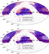 |
Fig. 1 Hammer–Aitoff equatorial projection of sky region binned (top panel) and Gaia G-band magnitude binned (bottom panel) reference samples. The blue scatters in the top and bottom panels represent the GoodQSO_Sky and GoodQSO_Mag, respectively. The red scatters in the top and bottom panels represent the GoodSTAR_Sky and GoodSTAR_Mag, respectively. |
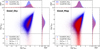 |
Fig. 2 log f0pm vs. log f0plx distributions of the Good_Sky (left panel) and Good_Mag (right panel), along with the quasar selection regions of the adopted astrometric criteria. The left panel shows the distributions of the sky-unbinned GoodQSO_Sky (blue points) and GoodSTAR_Sky (red points), while the right panel displays the corresponding distributions for the magnitude-unbinned GoodQSO_Mag (blue) and GoodSTAR_Mag (red). The black dotted dashed lines represent the f0pm criteria, while the dotted ones represent the f0plx criteria. All the histograms are normalized as probability density distributions (PDFs). Due to the long-tailed distributions of stars in log f0pm and log f0plx, i.e., many stars fall outside the plot range, both subplots display only small portions of the entire distributions. |
Astrometric criteria based on the Galactic latitude (b) and their corresponding completeness, purity, and stellar contamination.
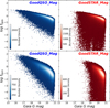 |
Fig. 4 log f0plx vs. Gaia G-band magnitude (top row) and log f0pm vs. Gaia G-band magnitude (bottom row) distributions of the GoodQSO_Mag (blue) and GoodSTAR_Mag (red). The color bar in each subplot represents the number density of the distribution. Note: the color map in each subplot follows its own color bar, and thus, identical colors across different subplots do not represent equivalent number densities. All the subplots display only small parts of the whole distributions to exhibit the critical data region. |
2.2.3 Visual inspection
The astrometric filtering isolates extragalactic sources along with a subset of stars exhibiting near-zero proper motions and parallaxes, yet it fails to distinguish galaxies from quasars. Therefore, MGQPCpreCAT still requires morphological inspection to exclude extended sources.
DESI-LS DR10 provides morphological classifications for all observed sources, including parameters denoted as PSF (point sources) and SER (Sersic surface brightness profiles). The MGQPCpreCAT was cross-matched with DR10 (ls_dr10.tractor catalog7) using a 1″ search radius to obtain morphological parameters of the candidates. The cross-matching yielded 2821 candidates with morphological parameters, the vast majority of which are classified as PSF. Although three major CSFs had been removed prior to the astrometric filtering in Section 2.2.2, a small number of candidates located in Galactic stellar clusters and spiral arms of nearby galaxies remained. Fortunately, these candidates are distinctly different from others and can be easily removed through visual inspection.
The g-, r-, and z-band imaging data of the MGQPCpreCAT sources were obtained from DESI-LS DR108 to support the visual inspection. Although DR10 covers nearly half of the entire sky (20 000 deg2), it lacks imaging data near the Galactic plane and in several specific sky areas. Therefore, the Pan-STARRS g-, r-, and z-band imaging data9 were used to supplement areas where DESI-LS DR10 images are either missing or of poor quality. All pseudo-color images were composited from g-, r-, and z-band images using HumVI (Marshall et al. 2015, 2016) via RGB combination.
With the support of morphological parameters and pseudocolor images, the visual inspection was performed on the 2821 candidates to exclude nearby galaxies, CSFs, and galaxies misclassified as PSF. The remaining 1465 candidates lacking morphological parameters were also visually inspected. Altogether, 174 CSFs and nearby galaxies were removed from the MGQPCpreCAT, with examples shown in Figure 6. A total of 4112 plausible quasar pair candidates were selected. We designate them as MGQPCs, which stands for “quasar pair candidates derived from the cross-match of MQC and Gaia”. The flowchart of the MGQPCs selection is shown in Figure 7.
Astrometric criteria based on the Gaia G-band magnitude (G) and their corresponding completeness, purity, and stellar contamination.
3 Overview of the MGQPC catalog
The basic statistical features of the final sample of quasar pair candidates (MGQPCs) and the advantages of the MGQPC catalog are described and validated in this section. Several fascinating pair systems are also described.
3.1 Basic features of MGQPCs
The comparison of the equatorial projection of the MGQPCpreCAT (left panel) and the visually selected MGQPCs (right panel) is displayed in Figure 8. Most MGQPCs are distributed in the northern hemisphere and visual inspection only induces minor variations in the number densities of several small regions. Figure 9 plots the MGQPCs’ Gaia G-band magnitude histogram (top panel) and distribution of the separation versus redshift (bottom panel). The redshifts are invoked from the known member quasars. Faint sources and moderately large separations dominate the MGQPC catalog, with a median Gaia G-band magnitude of 20.52 and a median member separation of 8.81″. The rapid decrease in the G-band magnitude histogram at G ≳ 20.8 mag is primarily due to missing or less precise astrometry at faint magnitudes (e.g., Section 3.1 and Figure 2 in Gaia Collaboration 2021). The number of MGQPCs decreases with increasing redshift and decreasing separation. Examples of MGQPCs are displayed in Figure 10. A description of the primary columns in the MGQPC catalog is given in Table 3.
To evaluate the color properties of the MGQPCs, a subset of 5000 quasars was randomly selected from GoodQSO_Mag. Nine types of color-color diagrams (e.g., Storey-Fisher et al. 2024; Fu et al. 2021, 2024, Fu et al. 2025) were applied, which incorporate multiband photometric data from PanSTARRS (grizy), AllWISE (W1, W2, and W3), and Gaia (G, BP, and RP). The distributions of the 5000 known quasars and the MGQPCs were overlaid on these diagrams (Figure 11). It should be noted that the number of MGQPCs varies across different color diagrams and is consistently smaller than the total number of MGQPCs due to missing multiband photometry for some candidates. In particular, diagrams involving AllWISE photometry contain only 700–800 MGQPCs. Nevertheless, they are still overlaid to partially reflect the color similarities or differences between the MGQPCs and known quasars. The color distribution of MGQPCs not only partially overlaps with known quasars but also exhibits stellar characteristics, such as the extended stripes and loci in the top row of the PanSTARRS color diagrams and obvious overdensities in other diagrams that do not coincide with quasar regions. Given the quasar selection efficiency of less than 70% obtained in Section 2.2.2, these distributions can be well explained. However, candidates that do not overlap with the quasar distribution could include potential new quasars disguised by stellar colors. Such quasars with anomalous colors are often missed by large surveys (e.g., SDSS) during target selection, while astrometric quasar selection can effectively retrieve them. Therefore, we argue that retaining them for subsequent spectroscopic follow-up is necessary.
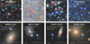 |
Fig. 6 Examples of visually rejected CSFs (top row) and morphologically removed nearby galaxies (bottom row). All these cutout images are obtained from DESI-LS DR10 grz bands and composited using HumVI. The blue and red circles with center points mark the quasars from MQCv8 and the astrometrically selected extragalactic candidates, respectively. Their Gaia G-band magnitudes, redshifts, and separation between them are denoted by Gmags(A,B), “zA,B”, and “sep”, respectively. All of these sources are unlikely quasar pairs and were removed. The size of each image is 30″ × 30″. North is up and east is to the left. |
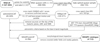 |
Fig. 7 Flowchart of the MGQPC catalog selection process. |
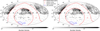 |
Fig. 8 Hammer–Aitoff projection of the MGQPCpreCAT (left panel) and the visually selected MGQPCs (right panel). On both panels, the red lines roughly demarcate the Galactic plane (0° ⩽ |b| < 20°), while the red cross and Y-shaped point mark the Galactic center and anti-center, respectively. The coverages of the LMC and SMC are bounded by the blue ellipses on both panels. |
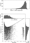 |
Fig. 9 Top panel: Gaia G-band magnitude histogram of the MGQPCs. Bottom panel: separation vs. redshift (the known quasar) of the MGQPCs. The solid line represents the 100 kpc criterion mentioned in Section 2.2.1. |
3.2 Advantages of the MGQPC catalog
To clarify the sample advantages of the MGQPCs, three recently published and relatively larger candidate quasar pair catalogs or catalogs containing a substantial number of quasar pair candidates are introduced here for comparison with the MGQPC catalog at three aspects (member separation, Gaia G-band magnitude, and redshift). The three catalogs are briefly described as follows:
A catalog of 436 multiply lensed and binary quasar candidates (875 individual sources) obtained by Dawes et al. (2023, hereafter, Dawes23) from the DESI-LS catalog by applying an autocorrelation algorithm.
A catalog of lensed quasar and quasar pair candidates, comprising 971 systems (1977 individual sources), compiled by He et al. (2023, hereafter, He23) based on the DESI-LS catalog and color similarity method.
A golden sample of 1867 dual quasar candidates derived by Wu et al. (2024, hereafter, Wu24) using the GMP technique.
All of these catalogs were recompiled in this work by crossmatching SIMBAD to update the redshifts and remove the newly confirmed pairs, as well as by cross-matching Gaia DR3 to retrieve the Gaia coordinates and G-band magnitudes of their members. The member separations were calculated according to the member coordinates. We note that the candidates in Wu24 are not pairs of Gaia sources, but single entries in Gaia DR3 with possible multiple components and most of them have spectroscopic or photometric redshifts, with only 298 candidates lacking a redshift determination. After our recompilation, there were 412, 994, and 1867 candidate quasar pairs in Dawes23, He23, and Wu24, respectively. In Dawes23, there are 830 individual sources with Gaia G-band magnitudes, while 150 systems have at least one member with spectroscopic redshifts. For He23, 1369 individual sources have Gaia G-band magnitudes, while 348 candidate pairs have at least one member with spectroscopic redshifts. And for Wu24, all the candidates have Gaia G-band magnitudes, while 1569 candidates have spectroscopic or photometric redshifts.
The comparative histograms of member separation, Gaia G-band magnitude, and redshift distributions are presented in Figure 12 for the three catalogs versus the MGQPCs. In terms of separation distribution (top panel), the Dawes23, He23, and MGQPCs cover ranges of 0.50″–4.99″, 0.50″–13.93″, and 0.66″–17.99″, respectively. The median separations of the three catalogs are 1.93″, 2.04″, and 8.81″, respectively. It should be noted that the separation distribution of Wu24 falls within Gaia’s resolution range for detecting multipeak sources (0.15″–0.80″), making its exact distribution and median value uncertain; thus, its distribution is not plotted in the histogram. The substantial difference in separation distribution and the higher median value of the MGQPC catalog suggest it is more suitable for expanding the quasar pair sample to larger separations, especially in the 5″–18″ range. For the magnitude distribution (middle panel), the Dawes23, He23, Wu24, and MGQPCs cover 16.15–21.60, 16.34–21.87, 14.96–20.50, and 16.34–21.00, respectively. Their median values are 20.12, 20.02, 19.66, and 20.52, indicating that the MGQPC catalog is slightly fainter and deeper than the other three catalogs. Finally, for the redshift distribution (bottom panel), the four catalogs cover 0.29–3.79, 0–3.80, 0–6.11, and 0.50–6.98, respectively. Their distribution characteristics are generally similar, and the median values are 1.67, 1.71, 1.25, and 1.61, respectively. However, there are still subtle differences: Dawes23 and He23 show higher fractions at z 1.5–2.5 than Wu24 and the MGQPC catalog, while Wu24 exhibits a significantly larger fraction at z ≲ 0.5 compared to the others. Furthermore, the MGQPC catalog shows marginally higher fractions at z 0.5–1.5 relative to the three catalogs. Moreover, compared to Wu24 (a dedicated dual quasar catalog), the MGQPC catalog contains significantly more sources at z 0.5–2.5. This suggests the MGQPC catalog might substantially augment more quasar pairs since cosmic noon (e.g., Shen et al. 2023b; Chen et al. 2023a; Gross et al. 2025).
On the other hand, the MGQPCs were cross-matched with the three catalogs, yielding 87 matches in Dawes23, 115 in He23, and 11 in Wu24. After excluding these matched candidates (totaling 128 candidate systems), 3984 new candidates were obtained, which had not been included in Dawes23, He23, or Wu24. This demonstrates that the MGQPCs provide a significantly complementary update to existing major candidate quasar pair catalogs, particularly in terms of member separation coverage.
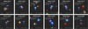 |
Fig. 10 Examples of MGQPCs. All these cutout images are obtained from DESI-LS DR10 grz bands and composited using HumVI. The marks of blue and red circles, text annotations, image size, and direction are the same as in Figure 6. |
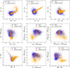 |
Fig. 11 Color features of the MGQPCs. The number of the MGQPCs in each color diagram is consistently smaller than the total number of MGQPCs due to missing multiband photometry for some candidates, while the number of QSOs is equal to 5000 in each diagram. All magnitudes are given in the AB system. |
Description of the primary columns in the MGQPC catalog.
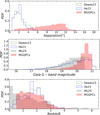 |
Fig. 12 Comparison of Dawes23 (green unfilled), He23 (blue unfilled), Wu24 (gray filled), and the MGQPC catalog (red filled) on the distributions of the member separation, Gaia G-band magnitude, and redshift. The y-axes are all scaled as probability distribution functions (PDF) to exhibit the distribution characteristics of the three parameters intuitively. Top panel: Separation histograms of Dawes23, He23, and the MGQPC catalog. Middle panel: Gaia G-band magnitude histograms of the four catalogs. Bottom panel: Redshift histograms of the four catalogs. |
3.3 Interesting candidates
The search for quasar pairs inevitably leads to the discovery of lensed quasars and vice versa (e.g., Agnello et al. 2018; Lemon et al. 2023; Yue et al. 2023; Dawes et al. 2023; Makarov & Secrest 2023; Ji et al. 2023, 2024). Currently, most confirmed lensed quasars have small separations, with the majority being within 4″. However, several wide-separation lensed quasars (WSLQs, e.g., Inada et al. 2003; Shu et al. 2018; Martinez et al. 2023; Napier et al. 2023) have also been discovered. These are typically the result of quasars being lensed by nearby galaxy groups or clusters. WSLQs can also occur when quasars are lensed by single galaxies, producing relatively large separations ranging from ~6″ to 10″. The largest separation of a WSLQ lensed by a single massive galaxy discovered to date is ~10.1″ (J1651-0417, also known as Dragon Kite, Ducourant et al. 2019; Stern et al. 2021; Connor et al. 2022).
During the visual inspection, we made note of some quasar pair candidates. Their relatively large separation, similar color, and configuration indicate the possibility of being potential WSLQs. These WSLQ candidates exhibit separations from ~6″ to 10″, with a potential galaxy located between them. Figure 13 displays three of these potential WSLQs. For comparison, the unique WSLQ lensed by a single massive galaxy, J1651-0417, is also displayed in Figure 13. Their multiband photometric data (via SED) were retrieved from the VizieR database10. Multiepoch measurements of the same band (if any) were averaged to characterize the photometry of that band.
The SEDs of the candidate quasars are highly similar to those of known quasars paired with them. This would indicate similar redshifts and spectral features such as the continuum and/or broad emission lines. Together with the existence of possible foreground galaxies, these systems might be WSLQs lensed by massive galaxies. However, they may also be quasargalaxy-quasar projection systems, which are precious natural laboratories of detailed study on the circumgalactic medium (e.g., Krishnarao et al. 2022).
4 Discussion
This section discusses potential reasons for the insensitivity of the astrometric criteria to sky regions described in Section 2.2.2, along with the astrometric efficiency, the reason for avoiding additional color cuts to further improve selection efficiency, and an approximate evaluation of stellar contamination in crowded fields. Finally, several techniques to improve the success rate of quasar pair candidate selection are discussed.
4.1 Quasar selection efficiency
The quasar selection purity, described in Section 2.2.2, remains invariant with Galactic latitude under identical astrometric criteria. Compared to Heintz20, we consider several potential reasons for this discrepancy. First, the astrometric criteria employed by Heintz20 differ slightly from ours: they utilized the signal-to-noise ratios of proper motion and parallax to characterize astrometric features; whereas we adopted the statistically more robust probability densities of zero proper motion and zero parallax. Second, Heintz20 relied on astrometric data from Gaia DR2 to assess selection efficiency, while we utilized the latest Gaia DR3, which may introduce subtle differences in the reference samples. Lastly, and most significantly, the selection of reference samples for quasars and stars differs. We constructed reference samples from the largest catalogs of spectroscopically confirmed quasars and stars that have Gaia DR3 astrometry. These reference samples are substantially augmented with newly confirmed quasars from SDSS DR18 and DESI DR1, particularly at low and intermediate Galactic latitudes. We assert that the reference samples selected in Section 2.2.2 exhibit higher completeness of sky distribution compared to those in Heintz20. Further validation may require a dedicated investigation.
Section 2.2.2 reports comprehensive purity and stellar contamination of 69.37% and 30.63%, respectively. We consider this astrometric selection purity an upper limit, as the actual purity may be further reduced by several factors. Since galaxies were not included in the reference samples despite their astrometric similarities to quasars, their presence may also reduce the quasar selection purity. Although the visual inspection described in Section 2.2.3 had removed some galaxies from the MGQPCpreCAT, we cannot unequivocally ensure the complete elimination of all galaxies. Furthermore, Figure 4 and Table 2 demonstrate that magnitude significantly affects astrometric quasar selection, particularly for candidates with G ⩾ 19. Therefore, the MGQPCs still contain approximately 31% stellar contamination, which could be mitigated by incorporating additional quasar selection techniques such as color cuts.
The color diagrams of the MGQPCs indicate that some candidates exhibit apparent stellar color features (Figure 11). These sources may be stellar contamination or could be quasars mimicking stellar colors. Such anomalous colors might result from interstellar and intergalactic reddening or interactions within quasar pairs. Applying color cuts may reduce the stellar contamination, but would also discard genuine quasars with unusual colors. Thus, we were able to preserve these candidates for subsequent follow-up confirmation. This is also the characteristic of this work: to search for quasars (and, hence, quasar pairs) that were missed by color selections.
Since pure astrometric techniques are unsuitable for CSFs, we removed candidates in the three major CSFs (totaling 11 482 objects) from the astrometricCAT before applying astrometric filtering in Section 2.2.2. Here, we provide a brief assessment of stellar contamination for these candidates. Color diagrams identical to those used for the MGQPCs are presented in Figure 14. The distribution of CSF candidates aligns closely with that of stars, indicating severe stellar contamination. Thus, quasar selection in CSFs remains challenging, even combining astrometric filtering and color cuts. It would be even more difficult to search for quasar pairs in these regions.
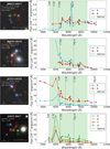 |
Fig. 13 Three potential WSLQs or quasar-galaxy-quasar projection systems noted during the visual inspection, as well as the J1651-0417. Their SEDs show the similarity between the members in each pair system, with several typical emission lines of the known quasars (black dashed lines with line names) and an optical wavelength region of 3000 Å– 9000 Å (green shaded area) overlapping on the SEDs. The marks and text annotations in the first three pseudo-color images are the same as in Figures 6 and 10, while the four colored circles with center points, along with “SepMax” and “zABCD” denote the quadruply lensed quasars, the largest separation in the J1651-0417 (occurs between A and D), and the redshift of this lensed quasar, respectively. |
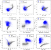 |
Fig. 14 Color features of CSFs. The number of CSFs in each color diagram is consistently smaller than the total CSFs due to missing multiband photometry for some candidates, while the number of QSOs is equal to 5000 in each diagram. All magnitudes are in the AB system. |
4.2 Future improvements
Although astrometric methods have been proven to be efficient in quasar searches in many studies, the search for quasar pairs not only requires the characteristic of zero proper motion and zero parallax, but also requires the redshifts of the two member quasars to be nearly identical. Therefore, more stringent criteria are still needed to refine the MGQPC catalog. To improve the success rate, several techniques might be helpful:
Estimating the photometric redshifts of the quasar candidates and selecting those with photometric redshifts similar to the spectroscopic redshifts of the nearby known quasars would be effective in selecting some high-confidence quasar pair candidates.
Avoiding sky coverages with small stellar proper motions could make sense when searching for quasar candidates with astrometric criteria, as this can make quasars more distinguishable from stars and reduce the stellar contamination. In addition, avoiding sky coverages of CSFs could also reduce stellar contamination.
Comparing the SEDs of the quasar candidates with those of the paired known quasars and selecting those pairs with high similarity in SEDs as high-probability quasar pair candidates would also work. We note that not all of their photometry across different bands was measured simultaneously, which would result in inaccurate SEDs. As a reference, and considering that the general variability of quasars is unlikely to change the features of their SEDs significantly, these photometric data can still be regarded as plausible and useful.
In the color-based quasar selection, some quasars lying just outside the selection boundaries may be omitted. These quasars with slightly anomalous colors can be easily isolated through astrometric methods (several newly discovered quasars lying just outside the boundaries will be reported in a forthcoming paper). Thus, using the astrometric method would be an effective quasar selection method to isolate sources that are near, but still outside of the quasar selection boundaries.
Since the fibers of existing spectroscopic surveys (e.g., SDSS, LAMOST, and DESI) have angular diameters of 1.5″–3″, those quasar pairs or lensed quasars with small separations (≲3″) cannot be resolved spatially in fiber spectroscopy and they might be identified as single quasars. Therefore, candidates with very small member separations can be set as high-priority.
Lastly, visual inspections can only remove nearby galaxies with apparent morphological characteristics, while removing high-redshift or morphologically uncharacteristic galaxies is difficult. Despite using morphological parameters from DESI-LS DR10, a small number of galaxies are still misclassified as point sources. Therefore, more precise morphological measurements are required to exclude galaxies with inactive nuclei and refine the quasar pair candidate sample.
5 Summary
In this work, we utilized the current largest quasar collection, Million Quasar Catalog, to perform a cross-matching with Gaia DR3 to systematically search for quasar pair candidates. The cross-matching radii were determined by a transverse distance of 100 kpc at the updated redshifts of the known quasars. Based on the reference samples of spectroscopically confirmed quasars and stars, multithreshold astrometric criteria based on the probability density were applied, isolating 4286 extragalactic candidates. A visual inspection was performed to remove CSFs and nearby galaxies. This resulted in 4112 candidates, which we designated as MGQPCs. Their median member separation is 8.81″, the Gaia G-band median magnitude is 20.52, and the median redshift is 1.61. The MGQPC catalog was compared with three major candidate quasar pair catalogs (Dawes23, He23, and Wu24) to demonstrate its advantages and complementary roles in constructing the quasar pair population. After excluding 128 duplicates shared with the three catalogs, 3984 previously uncataloged candidates were identified. Some WSLQ candidates were picked out during visual inspection and are briefly described. We also discuss our quasar selection purity of approximately 69%, as well as color properties of the MGQPCs and discarded candidates in the crowded fields. Several techniques for improving the success rate of quasar pair selection have been proposed, including photometric redshift estimation, sky coverage restriction, SED comparison, breaking of color methods, and unresolved quasar pairs in fiber spectroscopy. Approximately 31% of the MGQPC catalog contains residual stellar contaminants, necessitating extensive spectroscopic follow-up observations for validation.
A spectroscopic follow-up using Xinglong 2.16 m, Lijiang 2.4 m, Palomar 200-inch telescope (P200), and LAMOST-III was recently conducted for several tens of MGQPCs. The details of their observations and identifications will be reported in a follow-up paper.
Data availability
The MGQPC catalog is available at the CDS via https://cdsarc.cds.unistra.fr/viz-bin/cat/J/A+A/707/A30. Additionally, collaborative opportunities are open to conduct spectroscopic follow-up observations of the MGQPCs.
References
- Agnello, A., Schechter, P. L., Morgan, N. D., et al. 2018, MNRAS, 475, 2086 [Google Scholar]
- Almeida, A., Anderson, S. F., Argudo-Fernández, M., et al. 2023, ApJS, 267, 44 [NASA ADS] [CrossRef] [Google Scholar]
- Altamura, E., Brennan, S., Leśniewska, A., et al. 2020, AJ, 159, 122 [Google Scholar]
- An, T., Zhang, Y., Wang, A., et al. 2022, A&A, 663, A139 [NASA ADS] [CrossRef] [EDP Sciences] [Google Scholar]
- Antonucci, R. 1993, ARA&A, 31, 473 [Google Scholar]
- Astropy Collaboration (Robitaille, T. P., et al.) 2013, A&A, 558, A33 [NASA ADS] [CrossRef] [EDP Sciences] [Google Scholar]
- Astropy Collaboration (Price-Whelan, A. M., et al.) 2018, AJ, 156, 123 [Google Scholar]
- Astropy Collaboration (Price-Whelan, A. M., et al.) 2022, ApJ, 935, 167 [NASA ADS] [CrossRef] [Google Scholar]
- Begelman, M. C., Blandford, R. D., & Rees, M. J. 1980, Nature, 287, 307 [Google Scholar]
- Bolton, J. G., Peterson, B. A., Wills, B. J., & Wills, D. 1976, ApJ, 210, L1 [Google Scholar]
- Boroson, T. A., & Lauer, T. R. 2009, Nature, 458, 53 [Google Scholar]
- Bromley, B. C., Sandick, P., & Shams Es Haghi, B. 2024, Phys. Rev. D, 110, 023517 [Google Scholar]
- Chambers, K. C., Magnier, E. A., Metcalfe, N., et al. 2016, arXiv e-prints [arXiv:1612.05560] [Google Scholar]
- Charisi, M., Bartos, I., Haiman, Z., et al. 2016, MNRAS, 463, 2145 [Google Scholar]
- Chen, Y., Yu, Q., & Lu, Y. 2020, ApJ, 897, 86 [Google Scholar]
- Chen, Y.-C. 2021, MNRAS, submitted [arXiv:2109.06881] [Google Scholar]
- Chen, Y.-C., Hwang, H.-C., Shen, Y., et al. 2022, ApJ, 925, 162 [NASA ADS] [CrossRef] [Google Scholar]
- Chen, Y.-C., Liu, X., Foord, A., et al. 2023a, Nature, 616, 45 [NASA ADS] [CrossRef] [Google Scholar]
- Chen, Y.-C., Liu, X., Lazio, J., et al. 2023b, ApJ, 958, 29 [NASA ADS] [CrossRef] [Google Scholar]
- Chen, Y.-C., Gross, A. C., Liu, X., et al. 2025, ApJ, 988, 126 [Google Scholar]
- Ciurlo, A., Mannucci, F., Yeh, S., et al. 2023, A&A, 671, L4 [NASA ADS] [CrossRef] [EDP Sciences] [Google Scholar]
- Connor, T., Stern, D., Krone-Martins, A., et al. 2022, ApJ, 927, 45 [Google Scholar]
- Cui, X.-Q., Zhao, Y.-H., Chu, Y.-Q., et al. 2012, Res. Astron. Astrophys., 12, 1197 [Google Scholar]
- Davis, M. C., Grace, K. E., Trump, J. R., et al. 2024, ApJ, 965, 34 [Google Scholar]
- Dawes, C., Storfer, C., Huang, X., et al. 2023, ApJS, 269, 61 [NASA ADS] [CrossRef] [Google Scholar]
- de Bruijne, J. H. J. 2012, Ap & SS, 341, 31 [Google Scholar]
- De Rosa, A., Vignali, C., Bogdanović, T., et al. 2019, New A Rev., 86, 101525 [NASA ADS] [CrossRef] [Google Scholar]
- DESI Collaboration (Abdul-Karim, M., et al.) 2025, AJ, submitted [arXiv:2503.14745] [Google Scholar]
- Dey, A., Schlegel, D. J., Lang, D., et al. 2019, AJ, 157, 168 [Google Scholar]
- Djorgovski, S., Perley, R., Meylan, G., & McCarthy, P. 1987, ApJ, 321, L17 [Google Scholar]
- Du, P., & Wang, J.-M. 2023, A&A, 671, A26 [NASA ADS] [CrossRef] [EDP Sciences] [Google Scholar]
- Ducourant, C., Krone-Martins, A., Delchambre, L., et al. 2019, in SF2A-2019: Proceedings of the Annual meeting of the French Society of Astronomy and Astrophysics, eds. P. Di Matteo, O. Creevey, A. Crida, G. Kordopatis, J. Malzac, J. B. Marquette, M. N’Diaye, & O. Venot, Di [Google Scholar]
- Eracleous, M., Halpern, J. P., M. Gilbert, A., Newman, J. A., & Filippenko, A. V. 1997, ApJ, 490, 216 [NASA ADS] [CrossRef] [Google Scholar]
- Eracleous, M., Boroson, T. A., Halpern, J. P., & Liu, J. 2012a, ApJS, 201, 23 [Google Scholar]
- Eracleous, M., Flohic, H. M. L. G., & Bogdanović, T. 2012b, in Astronomical Society of the Pacific Conference Series, 460, AGN Winds in Charleston, eds. G. Chartas, F. Hamann, & K. M. Leighly, 214 [Google Scholar]
- Flesch, E. W. 2015, PASA, 32, e010 [Google Scholar]
- Flesch, E. W. 2023, Open J. Astrophys., 6, 49 [NASA ADS] [CrossRef] [Google Scholar]
- Foord, A., Gültekin, K., Nevin, R., et al. 2020, ApJ, 892, 29 [NASA ADS] [CrossRef] [Google Scholar]
- Fu, Y., Wu, X.-B., Yang, Q., et al. 2021, ApJS, 254, 6 [NASA ADS] [CrossRef] [Google Scholar]
- Fu, Y., Wu, X.-B., Li, Y., et al. 2024, ApJS, 271, 54 [NASA ADS] [CrossRef] [Google Scholar]
- Fu, Y., Wu, X.-B., Bouwens, R. J., et al. 2025, ApJS, 279, 54 [Google Scholar]
- Gaia Collaboration (Prusti, T., et al.) 2016, A&A, 595, A1 [NASA ADS] [CrossRef] [EDP Sciences] [Google Scholar]
- Gaia Collaboration (Brown, A. G. A., et al.) 2021, A&A, 649, A1 [NASA ADS] [CrossRef] [EDP Sciences] [Google Scholar]
- Gaia Collaboration (Vallenari, A., et al.) 2023, A&A, 674, A1 [NASA ADS] [CrossRef] [EDP Sciences] [Google Scholar]
- Graham, M. J., Djorgovski, S. G., Stern, D., et al. 2015a, MNRAS, 453, 1562 [Google Scholar]
- Graham, M. J., Djorgovski, S. G., Stern, D., et al. 2015b, Nature, 518, 74 [Google Scholar]
- Green, P. J., Myers, A. D., Barkhouse, W. A., et al. 2010, ApJ, 710, 1578 [Google Scholar]
- Gross, A. C., Chen, Y.-C., Oguri, M., et al. 2025, ApJ, 989, 112 [Google Scholar]
- Guo, H., Liu, X., Shen, Y., et al. 2019, MNRAS, 482, 3288 [Google Scholar]
- Harris, C. R., Millman, K. J., van der Walt, S. J., et al. 2020, Nature, 585, 357 [NASA ADS] [CrossRef] [Google Scholar]
- He, Z., Li, N., Cao, X., et al. 2023, A&A, 672, A123 [NASA ADS] [CrossRef] [EDP Sciences] [Google Scholar]
- He, Z., Chen, Q., Deng, L., et al. 2025, A&A, 695, A76 [NASA ADS] [CrossRef] [EDP Sciences] [Google Scholar]
- Heintz, K. E., Fynbo, J. P. U., & Høg, E. 2015, A&A, 578, A91 [NASA ADS] [CrossRef] [EDP Sciences] [Google Scholar]
- Heintz, K. E., Fynbo, J. P. U., Høg, E., et al. 2018, A&A, 615, L8 [NASA ADS] [CrossRef] [EDP Sciences] [Google Scholar]
- Heintz, K. E., Fynbo, J. P. U., Geier, S. J., et al. 2020, A&A, 644, A17 [NASA ADS] [CrossRef] [EDP Sciences] [Google Scholar]
- Hennawi, J. F., Strauss, M. A., Oguri, M., et al. 2006, AJ, 131, 1 [Google Scholar]
- Hennawi, J. F., Myers, A. D., Shen, Y., et al. 2010, ApJ, 719, 1672 [Google Scholar]
- Hou, M., Li, Z., & Liu, X. 2020, ApJ, 900, 79 [NASA ADS] [CrossRef] [Google Scholar]
- Hunter, J. D. 2007, Comput. Sci. Eng., 9, 90 [NASA ADS] [CrossRef] [Google Scholar]
- Hwang, H.-C., Shen, Y., Zakamska, N., & Liu, X. 2020, ApJ, 888, 73 [NASA ADS] [CrossRef] [Google Scholar]
- Impey, C. 1998, in Astronomical Society of the Pacific Conference Series, 146, The Young Universe: Galaxy Formation and Evolution at Intermediate and High Redshift, eds. S. D’Odorico, A. Fontana, & E. Giallongo, 391 [Google Scholar]
- Inada, N., Oguri, M., Pindor, B., et al. 2003, Nature, 426, 810 [NASA ADS] [CrossRef] [Google Scholar]
- Ji, X., Zheng, Z.-Y., Wu, Q., et al. 2023, MNRAS, 524, 1909 [CrossRef] [Google Scholar]
- Ji, X., Zheng, Z.-Y., Lin, R.-Q., & Feng, H.-C. 2024, ApJS, submitted, [arXiv:2412.08397] [Google Scholar]
- Kelley, L., Charisi, M., Burke-Spolaor, S., et al. 2019, BAAS, 51, 490 [Google Scholar]
- Kim, D., Im, M., Kim, M., & Ho, L. C. 2020a, ApJ, 894, 126 [NASA ADS] [CrossRef] [Google Scholar]
- Kim, D. C., Yoon, I., Evans, A. S., et al. 2020b, ApJ, 904, 23 [Google Scholar]
- Komossa, S., Burwitz, V., Hasinger, G., et al. 2003, ApJ, 582, L15 [NASA ADS] [CrossRef] [Google Scholar]
- Koo, D. C., Kron, R. G., & Cudworth, K. M. 1986, PASP, 98, 285 [Google Scholar]
- Koo, H., Bak, D., Park, I., Hong, S. E., & Lee, J.-W. 2024, Phys. Lett. B, 856, 138908 [Google Scholar]
- Krishnarao, D., Fox, A. J., D’Onghia, E., et al. 2022, Nature, 609, 915 [NASA ADS] [CrossRef] [Google Scholar]
- Lemon, C. A., Auger, M. W., McMahon, R. G., & Koposov, S. E. 2017, MNRAS, 472, 5023 [NASA ADS] [CrossRef] [Google Scholar]
- Lemon, C. A., Auger, M. W., & McMahon, R. G. 2019, MNRAS, 483, 4242 [NASA ADS] [CrossRef] [Google Scholar]
- Lemon, C., Anguita, T., Auger-Williams, M. W., et al. 2023, MNRAS, 520, 3305 [NASA ADS] [CrossRef] [Google Scholar]
- Liao, W.-T., Chen, Y.-C., Liu, X., et al. 2021, MNRAS, 500, 4025 [NASA ADS] [Google Scholar]
- Liu, Y. 2015, A&A, 580, A133 [NASA ADS] [CrossRef] [EDP Sciences] [Google Scholar]
- Liu, Y. 2016, A&A, 592, L4 [NASA ADS] [CrossRef] [EDP Sciences] [Google Scholar]
- Liu, F. K., Wu, X.-B., & Cao, S. L. 2003, MNRAS, 340, 411 [NASA ADS] [CrossRef] [Google Scholar]
- Liu, X., Shen, Y., Strauss, M. A., & Hao, L. 2011, ApJ, 737, 101 [Google Scholar]
- Lyke, B. W., Higley, A. N., McLane, J. N., et al. 2020, ApJS, 250, 8 [NASA ADS] [CrossRef] [Google Scholar]
- Makarov, V. V., & Secrest, N. J. 2022, ApJ, 933, 28 [NASA ADS] [CrossRef] [Google Scholar]
- Makarov, V. V., & Secrest, N. J. 2023, ApJS, 264, 4 [Google Scholar]
- Makarov, V., Berghea, C., Boboltz, D., et al. 2012, Mem. Soc. Astron. Italiana, 83, 952 [NASA ADS] [Google Scholar]
- Mannucci, F., Pancino, E., Belfiore, F., et al. 2022, Nat. Astron., 6, 1185 [NASA ADS] [CrossRef] [Google Scholar]
- Mannucci, F., Scialpi, M., Ciurlo, A., et al. 2023, A&A, 680, A53 [NASA ADS] [CrossRef] [EDP Sciences] [Google Scholar]
- Marshall, P., Sandford, C., More, A., & Buddelmeijerr, H. 2015, HumVI: Human Viewable Image creation, Astrophysics Source Code Library [record ascl:1511.014] [Google Scholar]
- Marshall, P. J., Verma, A., More, A., et al. 2016, MNRAS, 455, 1171 [NASA ADS] [CrossRef] [Google Scholar]
- Martinez, M. N., Napier, K. A., Cloonan, A. P., et al. 2023, ApJ, 946, 63 [NASA ADS] [CrossRef] [Google Scholar]
- Merritt, D. 2013, Dynamics and Evolution of Galactic Nuclei [Google Scholar]
- Merritt, D., & Milosavljević, M. 2005, Liv. Rev. Relativ., 8, 8 [Google Scholar]
- Meylan, G., Djorgovski, S., Perley, R., & McCarthy, P. 1987, The Messenger, 48, 34 [Google Scholar]
- Milosavljević, M., & Merritt, D. 2001, ApJ, 563, 34 [Google Scholar]
- Muñoz, J. A., Falco, E. E., Kochanek, C. S., et al. 1998, ApJ, 492, L9 [Google Scholar]
- Myers, A. D., Richards, G. T., Brunner, R. J., et al. 2008, ApJ, 678, 635 [Google Scholar]
- Napier, K., Gladders, M. D., Sharon, K., et al. 2023, ApJ, 954, L38 [NASA ADS] [CrossRef] [Google Scholar]
- Netzer, H. 2015, ARA&A, 53, 365 [Google Scholar]
- pandas development team, T. 2022, pandas-dev/pandas: Pandas [Google Scholar]
- Pfeifle, R. W., Weaver, K. A., Secrest, N. J., Rothberg, B., & Patton, D. R. 2025, ApJS, 281, 25 [Google Scholar]
- Richarte, M. G., Toscano, F., Garcia Lambas, D., et al. 2025, A&A, 700, A269 [NASA ADS] [CrossRef] [EDP Sciences] [Google Scholar]
- Ross, N. P., Myers, A. D., Sheldon, E. S., et al. 2012, ApJS, 199, 3 [NASA ADS] [CrossRef] [Google Scholar]
- Sandage, A. 1965, ApJ, 141, 1560 [NASA ADS] [CrossRef] [Google Scholar]
- Sandrinelli, A., Falomo, R., Treves, A., Farina, E. P., & Uslenghi, M. 2014, MNRAS, 444, 1835 [Google Scholar]
- Sandrinelli, A., Falomo, R., Treves, A., Scarpa, R., & Uslenghi, M. 2018, MNRAS, 474, 4925 [NASA ADS] [CrossRef] [Google Scholar]
- Schmidt, M. 1963, Nature, 197, 1040 [Google Scholar]
- Schwartzman, E., Clarke, T. E., Nyland, K., et al. 2024, ApJ, 961, 233 [NASA ADS] [Google Scholar]
- Scialpi, M., Mannucci, F., Marconcini, C., et al. 2024, A&A, 690, A57 [NASA ADS] [CrossRef] [EDP Sciences] [Google Scholar]
- Shen, Y., & Loeb, A. 2010, ApJ, 725, 249 [NASA ADS] [CrossRef] [Google Scholar]
- Shen, Y., Hennawi, J. F., Shankar, F., et al. 2010, ApJ, 719, 1693 [NASA ADS] [CrossRef] [Google Scholar]
- Shen, Y., Hwang, H.-C., Zakamska, N., & Liu, X. 2019, ApJ, 885, L4 [NASA ADS] [CrossRef] [Google Scholar]
- Shen, Y., Chen, Y.-C., Hwang, H.-C., et al. 2021, Nat. Astron., 5, 569 [NASA ADS] [CrossRef] [Google Scholar]
- Shen, Y., Casey-Clyde, J. A., Chen, Y.-C., et al. 2023a, arXiv e-prints [arXiv:2306.15527] [Google Scholar]
- Shen, Y., Hwang, H.-C., Oguri, M., et al. 2023b, ApJ, 943, 38 [NASA ADS] [CrossRef] [Google Scholar]
- Shu, Y., Marques-Chaves, R., Evans, N. W., & Pérez-Fournon, I. 2018, MNRAS, 481, L136 [Google Scholar]
- Shu, Y., Koposov, S. E., Evans, N. W., et al. 2019, MNRAS, 489, 4741 [Google Scholar]
- Sillanpää, A., Haarala, S., Valtonen, M. J., Sundelius, B., & Byrd, G. G. 1988, ApJ, 325, 628 [NASA ADS] [CrossRef] [Google Scholar]
- Silverman, J. D., Tang, S., Lee, K.-G., et al. 2020, ApJ, 899, 154 [Google Scholar]
- Souchay, J., Secrest, N., Lambert, S., et al. 2022, A&A, 660, A16 [NASA ADS] [CrossRef] [EDP Sciences] [Google Scholar]
- Stern, D., Djorgovski, S. G., Krone-Martins, A., et al. 2021, ApJ, 921, 42 [NASA ADS] [CrossRef] [Google Scholar]
- Stockton, A. N. 1972, Nat. Phys. Sci., 238, 37 [Google Scholar]
- Storey-Fisher, K., Hogg, D. W., Rix, H.-W., et al. 2024, ApJ, 964, 69 [NASA ADS] [CrossRef] [Google Scholar]
- Tang, S., & Grindlay, J. 2009, ApJ, 704, 1189 [NASA ADS] [CrossRef] [Google Scholar]
- Tang, S., Silverman, J. D., Ding, X., et al. 2021, ApJ, 922, 83 [NASA ADS] [CrossRef] [Google Scholar]
- Taylor, M. B. 2005, in Astronomical Society of the Pacific Conference Series, 347, Astronomical Data Analysis Software and Systems XIV, eds. P. Shopbell, M. Britton, & R. Ebert, 29 [NASA ADS] [Google Scholar]
- Uppal, A., Ward, C., Gezari, S., et al. 2024, ApJ, 975, 286 [Google Scholar]
- Urry, C. M., & Padovani, P. 1995, PASP, 107, 803 [NASA ADS] [CrossRef] [Google Scholar]
- van der Walt, S., Colbert, S. C., & Varoquaux, G. 2011, Comput. Sci. Eng., 13, 22 [Google Scholar]
- Wampler, E. J., Baldwin, J. A., Burke, W. L., & Robinson, L. B. 1973, Nature, 246, 203 [Google Scholar]
- Wang, H.-C., Wang, J.-X., Gu, M.-F., & Liao, M. 2023a, MNRAS, 524, L38 [Google Scholar]
- Wang, J.-M., Songsheng, Y.-Y., Li, Y.-R., & Du, P. 2023b, MNRAS, 518, 3397 [Google Scholar]
- Wenger, M., Ochsenbein, F., Egret, D., et al. 2000, A&AS, 143, 9 [NASA ADS] [Google Scholar]
- Wes McKinney 2010, in Proceedings of the 9th Python in Science Conference, eds. S. van der Walt, & J. Millman, 56 [Google Scholar]
- Wright, E. L., Eisenhardt, P. R. M., Mainzer, A. K., et al. 2010, AJ, 140, 1868 [Google Scholar]
- Wu, X.-B., Hao, G., Jia, Z., Zhang, Y., & Peng, N. 2012, AJ, 144, 49 [Google Scholar]
- Wu, Q.-Q., Liao, S.-L., Ji, X., et al. 2022, Front. Astron. Space Sci., 9, 822768 [NASA ADS] [CrossRef] [Google Scholar]
- Wu, Q., Liao, S., Qi, Z., et al. 2023, Res. Astron. Astrophys., 23, 025006 [Google Scholar]
- Wu, Q., Scialpi, M., Liao, S., Mannucci, F., & Qi, Z. 2024, A&A, 692, A154 [NASA ADS] [CrossRef] [EDP Sciences] [Google Scholar]
- Xu, W., Cui, L., Liu, X., et al. 2024, ApJ, 969, 36 [NASA ADS] [CrossRef] [Google Scholar]
- Yan, C.-S., Lu, Y., Dai, X., & Yu, Q. 2015, ApJ, 809, 117 [Google Scholar]
- Yèche, C., Palanque-Delabrouille, N., Claveau, C.-A., et al. 2020, RNAAS, 4, 179 [Google Scholar]
- York, D. G., Adelman, J., Anderson, John E., J., et al. 2000, AJ, 120, 1579 [NASA ADS] [CrossRef] [Google Scholar]
- Yu, Q. 2002, MNRAS, 331, 935 [Google Scholar]
- Yue, M., Fan, X., Yang, J., & Wang, F. 2023, AJ, 165, 191 [NASA ADS] [CrossRef] [Google Scholar]
- Zhang, F. 2023, arXiv e-prints [arXiv:2312.11847] [Google Scholar]
- Zheng, Q., Liu, S., Zhang, X., & Yuan, Q. 2023, ApJ, 944, 4 [Google Scholar]
- Zheng, Q., Zhang, X., Yuan, Q., Severgnini, P., & Vignali, C. 2024, MNRAS, 531, L76 [Google Scholar]
- Zhou, H., Wang, T., Zhang, X., Dong, X., & Li, C. 2004, ApJ, 604, L33 [NASA ADS] [CrossRef] [Google Scholar]
MILLIQUAS v8.0 (2023) update, https://heasarc.gsfc.nasa.gov/W3Browse/all/milliquas.html
Appendix A Acknowledgments
The authors thank the anonymous referee for the valuable comments that improved the quality and clarity of the manuscript. The authors thank Qirong Yuan, Heng Yu, He Gao, Yiping Shu, Xikai Shan, Yuming Fu, and Yuanzhen Han for their suggestions and guidance on several details. This work has been supported by the Chinese National Natural Science Foundation grant No. 12333001 and by the National Key R&D Program of China (2021YFA0718500 and 2025YFA1614101).
This work has made use of data from the European Space Agency (ESA) mission Gaia (https://www.cosmos.esa.int/gaia), processed by the Gaia Data Processing and Analysis Consortium (DPAC, https://www.cosmos.esa.int/web/gaia/dpac/consortium). Funding for the DPAC has been provided by national institutions, in particular the institutions participating in the Gaia Multilateral Agreement.
Funding for the Sloan Digital Sky Survey V has been provided by the Alfred P. Sloan Foundation, the Heising-Simons Foundation, the National Science Foundation, and the Participating Institutions. SDSS acknowledges support and resources from the Center for High-Performance Computing at the University of Utah. SDSS telescopes are located at Apache Point Observatory, funded by the Astrophysical Research Consortium and operated by New Mexico State University, and at Las Campanas Observatory, operated by the Carnegie Institution for Science. The SDSS website is www.sdss.org.
Guoshoujing Telescope (the Large Sky Area Multi-Object Fiber Spectroscopic Telescope, LAMOST) is a National Major Scientific Project built by the Chinese Academy of Sciences. Funding for the project has been provided by the National Development and Reform Commission. LAMOST is operated and managed by the National Astronomical Observatories, Chinese Academy of Sciences.
This research used data obtained with the Dark Energy Spectroscopic Instrument (DESI). DESI construction and operations are managed by the Lawrence Berkeley National Laboratory. This material is based upon work supported by the U.S. Department of Energy, Office of Science, Office of High-Energy Physics, under Contract No. DE–AC02–05CH11231, and by the National Energy Research Scientific Computing Center, a DOE Office of Science User Facility under the same contract. Additional support for DESI was provided by the U.S. National Science Foundation (NSF), Division of Astronomical Sciences under Contract No. AST-0950945 to the NSF’s National Optical-Infrared Astronomy Research Laboratory; the Science and Technology Facilities Council of the United Kingdom; the Gordon and Betty Moore Foundation; the Heising-Simons Foundation; the French Alternative Energies and Atomic Energy Commission (CEA); the National Council of Humanities, Science and Technology of Mexico (CONAHCYT); the Ministry of Science and Innovation of Spain (MICINN), and by the DESI Member Institutions: www.desi.lbl.gov/collaborating-institutions. The DESI collaboration is honored to be permitted to conduct scientific research on I’oligam Du’ag (Kitt Peak), a mountain with particular significance to the Tohono O’odham Nation. Any opinions, findings, and conclusions or recommendations expressed in this material are those of the author(s) and do not necessarily reflect the views of the U.S. National Science Foundation, the U.S. Department of Energy, or any of the listed funding agencies.
The DESI Legacy Imaging Surveys consist of three individual and complementary projects: the Dark Energy Camera Legacy Survey (DECaLS), the Beijing-Arizona Sky Survey (BASS), and the Mayall z-band Legacy Survey (MzLS). Pipeline processing and analyses of the data were supported by NOIRLab and the Lawrence Berkeley National Laboratory (LBNL). Legacy Surveys was supported by: the Director, Office of Science, Office of High Energy Physics of the U.S. Department of Energy; the National Energy Research Scientific Computing Center, a DOE Office of Science User Facility; the U.S. National Science Foundation, Division of Astronomical Sciences; the National Astronomical Observatories of China, the Chinese Academy of Sciences and the Chinese National Natural Science Foundation. LBNL is managed by the Regents of the University of California under contract to the U.S. Department of Energy.
The Pan-STARRS1 Surveys (PS1) and the PS1 public science archive have been made possible through contributions by the Institute for Astronomy, the University of Hawaii, the Pan-STARRS Project Office, the Max-Planck Society and its participating institutes, the Max Planck Institute for Astronomy, Heidelberg and the Max Planck Institute for Extraterrestrial Physics, Garching, The Johns Hopkins University, Durham University, the University of Edinburgh, the Queen’s University Belfast, the Harvard-Smithsonian Center for Astrophysics, the Las Cumbres Observatory Global Telescope Network Incorporated, the National Central University of Taiwan, the Space Telescope Science Institute, the National Aeronautics and Space Administration under Grant No. NNX08AR22G issued through the Planetary Science Division of the NASA Science Mission Directorate, the National Science Foundation Grant No. AST–1238877, the University of Maryland, Eotvos Lorand University (ELTE), the Los Alamos National Laboratory, and the Gordon and Betty Moore Foundation.
We acknowledge the use of public data from the following facilities: Gaia, SDSS, LAMOST, DESI, DESI Legacy Survey, and Pan-STARRS. This research made use of the following software packages: Astropy (Astropy Collaboration 2013, 2018, 2022), Matplotlib (Hunter 2007), NumPy (van der Walt et al. 2011; Harris et al. 2020), Pandas (Wes McKinney 2010; pandas development team 2022), TOPCAT (Taylor 2005), HumVI (Marshall et al. 2015, Marshall et al. 2016).
All Tables
Astrometric criteria based on the Galactic latitude (b) and their corresponding completeness, purity, and stellar contamination.
Astrometric criteria based on the Gaia G-band magnitude (G) and their corresponding completeness, purity, and stellar contamination.
All Figures
|
Fig. 1 Hammer–Aitoff equatorial projection of sky region binned (top panel) and Gaia G-band magnitude binned (bottom panel) reference samples. The blue scatters in the top and bottom panels represent the GoodQSO_Sky and GoodQSO_Mag, respectively. The red scatters in the top and bottom panels represent the GoodSTAR_Sky and GoodSTAR_Mag, respectively. |
| In the text | |
|
Fig. 2 log f0pm vs. log f0plx distributions of the Good_Sky (left panel) and Good_Mag (right panel), along with the quasar selection regions of the adopted astrometric criteria. The left panel shows the distributions of the sky-unbinned GoodQSO_Sky (blue points) and GoodSTAR_Sky (red points), while the right panel displays the corresponding distributions for the magnitude-unbinned GoodQSO_Mag (blue) and GoodSTAR_Mag (red). The black dotted dashed lines represent the f0pm criteria, while the dotted ones represent the f0plx criteria. All the histograms are normalized as probability density distributions (PDFs). Due to the long-tailed distributions of stars in log f0pm and log f0plx, i.e., many stars fall outside the plot range, both subplots display only small portions of the entire distributions. |
| In the text | |
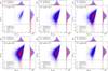 |
Fig. 3 Same as the left panel of Figure 2, but for the Good_Sky at different Galactic latitude bins. |
| In the text | |
|
Fig. 4 log f0plx vs. Gaia G-band magnitude (top row) and log f0pm vs. Gaia G-band magnitude (bottom row) distributions of the GoodQSO_Mag (blue) and GoodSTAR_Mag (red). The color bar in each subplot represents the number density of the distribution. Note: the color map in each subplot follows its own color bar, and thus, identical colors across different subplots do not represent equivalent number densities. All the subplots display only small parts of the whole distributions to exhibit the critical data region. |
| In the text | |
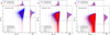 |
Fig. 5 Similar to Figure 3, but for the Good_Mag at different Gaia G-band magnitude bins. |
| In the text | |
|
Fig. 6 Examples of visually rejected CSFs (top row) and morphologically removed nearby galaxies (bottom row). All these cutout images are obtained from DESI-LS DR10 grz bands and composited using HumVI. The blue and red circles with center points mark the quasars from MQCv8 and the astrometrically selected extragalactic candidates, respectively. Their Gaia G-band magnitudes, redshifts, and separation between them are denoted by Gmags(A,B), “zA,B”, and “sep”, respectively. All of these sources are unlikely quasar pairs and were removed. The size of each image is 30″ × 30″. North is up and east is to the left. |
| In the text | |
|
Fig. 7 Flowchart of the MGQPC catalog selection process. |
| In the text | |
|
Fig. 8 Hammer–Aitoff projection of the MGQPCpreCAT (left panel) and the visually selected MGQPCs (right panel). On both panels, the red lines roughly demarcate the Galactic plane (0° ⩽ |b| < 20°), while the red cross and Y-shaped point mark the Galactic center and anti-center, respectively. The coverages of the LMC and SMC are bounded by the blue ellipses on both panels. |
| In the text | |
|
Fig. 9 Top panel: Gaia G-band magnitude histogram of the MGQPCs. Bottom panel: separation vs. redshift (the known quasar) of the MGQPCs. The solid line represents the 100 kpc criterion mentioned in Section 2.2.1. |
| In the text | |
|
Fig. 10 Examples of MGQPCs. All these cutout images are obtained from DESI-LS DR10 grz bands and composited using HumVI. The marks of blue and red circles, text annotations, image size, and direction are the same as in Figure 6. |
| In the text | |
|
Fig. 11 Color features of the MGQPCs. The number of the MGQPCs in each color diagram is consistently smaller than the total number of MGQPCs due to missing multiband photometry for some candidates, while the number of QSOs is equal to 5000 in each diagram. All magnitudes are given in the AB system. |
| In the text | |
|
Fig. 12 Comparison of Dawes23 (green unfilled), He23 (blue unfilled), Wu24 (gray filled), and the MGQPC catalog (red filled) on the distributions of the member separation, Gaia G-band magnitude, and redshift. The y-axes are all scaled as probability distribution functions (PDF) to exhibit the distribution characteristics of the three parameters intuitively. Top panel: Separation histograms of Dawes23, He23, and the MGQPC catalog. Middle panel: Gaia G-band magnitude histograms of the four catalogs. Bottom panel: Redshift histograms of the four catalogs. |
| In the text | |
|
Fig. 13 Three potential WSLQs or quasar-galaxy-quasar projection systems noted during the visual inspection, as well as the J1651-0417. Their SEDs show the similarity between the members in each pair system, with several typical emission lines of the known quasars (black dashed lines with line names) and an optical wavelength region of 3000 Å– 9000 Å (green shaded area) overlapping on the SEDs. The marks and text annotations in the first three pseudo-color images are the same as in Figures 6 and 10, while the four colored circles with center points, along with “SepMax” and “zABCD” denote the quadruply lensed quasars, the largest separation in the J1651-0417 (occurs between A and D), and the redshift of this lensed quasar, respectively. |
| In the text | |
|
Fig. 14 Color features of CSFs. The number of CSFs in each color diagram is consistently smaller than the total CSFs due to missing multiband photometry for some candidates, while the number of QSOs is equal to 5000 in each diagram. All magnitudes are in the AB system. |
| In the text | |
Current usage metrics show cumulative count of Article Views (full-text article views including HTML views, PDF and ePub downloads, according to the available data) and Abstracts Views on Vision4Press platform.
Data correspond to usage on the plateform after 2015. The current usage metrics is available 48-96 hours after online publication and is updated daily on week days.
Initial download of the metrics may take a while.