| Issue |
A&A
Volume 707, March 2026
|
|
|---|---|---|
| Article Number | A92 | |
| Number of page(s) | 22 | |
| Section | Stellar atmospheres | |
| DOI | https://doi.org/10.1051/0004-6361/202556207 | |
| Published online | 12 March 2026 | |
Clouds and chemistry across the brown dwarf T-Y sequence: Insights from JWST atmospheric retrievals
1
Faculty of Physics, Ludwig Maximilian University,
Scheinerstrasse 1,
81679
Munich,
Bavaria,
Germany
2
Center for Space and Habitability, University of Bern,
Gesellschaftsstrasse 6,
3012
Bern,
Switzerland
3
Space Research and Planetary Sciences, Physics Institute, University of Bern,
Gesellschaftsstrasse 6,
3012
Bern,
Switzerland
4
ARTORG Center for Biomedical Engineering Research, University of Bern,
Murtenstrasse 50,
3008
Bern,
Switzerland
5
University College London, Department of Physics & Astronomy,
Gower St,
London
WC1E 6BT,
UK
6
Astronomy & Astrophysics Group, Department of Physics, University of Warwick,
Coventry
CV4 7AL,
UK
★ Corresponding author: This email address is being protected from spambots. You need JavaScript enabled to view it.
Received:
1
July
2025
Accepted:
16
January
2026
Abstract
The James Webb Space Telescope offers exceptional spectral resolution and wavelength coverage, which are essential for studying the coldest brown dwarfs, particularly Y dwarfs. These objects are at the cold end of the substellar sequence and exhibit atmospheric phenomena such as cloud formation, chemical disequilibrium, and radiative-convective coupling. We examined a curated sample of 22 late-T to Y dwarfs through Bayesian atmospheric retrieval (nested sampling) and supervised machine learning (random forests). Our Bayesian model comparison indicates that cloud-free models are generally favored for the hottest objects in the sample (T6-T8). Conversely, later-type dwarfs exhibit varying preferences, with both gray cloud and cloud-free models providing comparable fits. The atmospheric parameters retrieved are consistent across the applied methodologies. Evidence of vertical mixing and disequilibrium chemistry is found in several objects; notably, the Y1 dwarf WISEPAJ1541-22 favors a gray cloud model and shows elevated abundances of both CO and CO2 compared to equilibrium chemistry calculations. As anticipated, the abundances of H2O, CH4, and NH3 increase with decreasing effective temperature over the T-Y sequence.
Key words: techniques: spectroscopic / planets and satellites: atmospheres / planets and satellites: composition / brown dwarfs
© The Authors 2026
 Open Access article, published by EDP Sciences, under the terms of the Creative Commons Attribution License (https://creativecommons.org/licenses/by/4.0), which permits unrestricted use, distribution, and reproduction in any medium, provided the original work is properly cited.
This article is published in open access under the Subscribe to Open model. This email address is being protected from spambots. You need JavaScript enabled to view it. to support open access publication.
1 Introduction
The study of brown dwarfs has been greatly facilitated by the accumulation of a large amount of spectral data in recent years. Numerous observational campaigns have been conducted using ground-based and space-based telescopes, resulting in a wealth of information about the spectra of these objects (see, e.g., Kirkpatrick et al. 2021). This large amount of data has motivated several population studies whose purpose is to gain a holistic understanding of the atmospheres of brown dwarfs (Line et al. 2015, 2017; Burningham et al. 2017; Zalesky et al. 2019, 2022; Gonzales et al. 2020, 2022; Lueber et al. 2022; Calamari et al. 2024). However, these efforts have so far been constrained by the existing limitations in data quality and near-infrared wavelength coverage. In the investigation conducted by Lueber et al. (2022), a comprehensive examination of brown dwarfs spanning the entire L-T spectral sequence was carried out using 19 SpeX Prism spectral standards (Burgasser 2014). Despite thorough analysis, some important research questions remained unanswered. For instance, the absence of a preference for cloudy models in the case of L dwarfs was unexpected, with both cloud-free and cloudy models appearing to be equally consistent with the archival SpeX data from the perspective of Bayesian model comparison. A primary contributing factor to this ambiguity could be attributed to the restricted wavelength coverage of SpeX spectroscopy.
The launch of the James Webb Space Telescope (JWST; Gardner et al. 2023) has helped shift these limitations. The instruments on board JWST enable a major advance in spectral resolution and wavelength coverage, which are crucial for the coldest brown dwarfs due to their very low temperatures and faintness in the near-infrared. This study aims to expand the analysis performed by Lueber et al. (2022) to the colder Y dwarf regime, which represents the coldest and least understood members of the brown dwarf population. We utilized the curated data set of Beiler et al. (2024a), who observed 23 brown dwarfs with the near-infrared spectrograph (NIRSpec; Jakobsen et al. 2022) and the mid-infrared instrument (MIRI; Rieke et al. 2015) of JWST and collected low-resolution spectroscopy with both instruments and broadband photometry with MIRI (GO 2302, PI: Cushing).
The Y dwarfs are crucial for understanding the lower temperature limits of substellar atmospheres, where the interplay of complex processes such as cloud formation, chemical disequilibrium, and radiative-convective dynamics become dominant (Cushing et al. 2011; Kirkpatrick et al. 2012; Morley et al. 2012, 2014; Lacy & Burrows 2023; Leggett & Tremblin 2023; Leggett 2024). To address these complexities, we utilized standard Bayesian nested-sampling atmospheric retrieval techniques (Kitzmann et al. 2020) across the T-Y spectral sequence, which is analogous to the approach taken by Lueber et al. (2022). Additionally, we compared our nested-sampling retrievals with those performed using the supervised machine learning-based random forest method (Márquez-Neila et al. 2018). This method offers a data-driven approach that complements traditional Bayesian analysis, allowing us to explore the predictive power of different atmospheric features in a non-parametric fashion.
Machine learning approaches such as random forests facilitate an additional layer of analysis through the concept of “feature importance” (Márquez-Neila et al. 2018), which quantifies the relative contribution of each input feature-in this case, each data point across wavelength-to the prediction of a given model parameter. We present an analysis of feature importance using a custom model grid constructed for this study. By evaluating which wavelengths contribute most significantly to the model parameter predictions (e.g., temperature or chemical abundances), we can gain deeper insights into the physical processes governing Y dwarf atmospheres. This feature importance analysis helps highlight key factors that may have been overlooked in prior studies, especially when dealing with the more complex, cooler atmospheric conditions found in Y dwarfs. Thus, by combining the Bayesian and random forest retrieval analysis, we aim to resolve some of the ambiguities identified in earlier work and to contribute to a more comprehensive understanding of the substellar population.
Set of brown dwarfs and their observational characteristics used in this study.
2 Spectral sample
For this study, we used the curated dataset from Beiler et al. (2024a), which includes observations of 23 brown dwarfs with JWST’s NIRSpec (Jakobsen et al. 2022) and MIRI (Rieke et al. 2015). This dataset provides low-resolution spectroscopy from both instruments, covering the ~1-12 μm wavelength range at λ∕∆λ ≈ 100 (GO 2302, PI: Cushing). The data were not reprocessed. For a detailed description of the reduction procedures, we refer to Beiler et al. (2024a). WISEPA J2018-74 (T7) lacks NIRSpec observations and is therefore excluded from our analysis. Our set of 22 brown dwarfs are shown in Fig. 1, and their known properties are given in Table 1.
3 Atmospheric retrieval approach
3.1 Bayesian framework
In this investigation, we employed the open-source Bern Atmospheric Retrieval (BEAR) code, which is an updated version of the earlier Helios-r2 code described by Kitzmann et al. (2020). BEAR features enhanced capabilities and additional forward models. For our analysis, we used the emission spectroscopy forward model available in BEAR. The code and comprehensive documentation are publicly accessible under the GNU General Public License and can be found on GitHub1. BEAR incorporates the MultiNest (Feroz & Hobson 2008; Feroz et al. 2009) algorithm for Bayesian nested sampling (Skilling 2004, 2006) to explore the multi-dimensional parameter space of the models, compute posterior distributions, and calculate the Bayesian evidence. For this study, we employed the emission spectroscopy forward model of BEAR, which, as originally presented by Kitzmann et al. (2020), solves the radiative transfer equation by using the short characteristics method as described by Olson & Kunasz (1987).
The one-dimensional, plane-parallel model atmosphere comprises 99 layers (100 levels) extending from 100 bar to 1 mbar. The temperature-pressure profile is characterized by a finite element approach that ensures smoothness and continuity (Kitzmann et al. 2020). In the current study, it is described by two regimes.
The radiative-convective boundary (RCB) was parameterized, defining the depth at which the atmosphere transitions from being dominated by convective energy transport in deeper atmospheric layers to being dominated by radiative energy transport. Below the RCB (at higher pressures), the thermal profile is described by following an adiabatic gradient determined by the adiabatic index:
 (1)
(1)
Here, cp and cv are the heat capacities at constant pressure and at constant volume, respectively. The number of degrees of freedom are denoted as n. We approximated the adiabatic temperature-pressure profile as
 (2)
(2)
Assuming a constant value of γ, we could thus neglect the potential temperature dependence of cp and cV. The constant value of γ, however, still depends on the chemical composition and degrees of freedom of the gas. For an ideal diatomic gas such as molecular hydrogen (H2), γ = 7/5 = 1.4, whereas for monatomic gases, γ = 5/3 ≈ 1.67. The γ and the RCB parameters are both treated as free parameters of the model.
The adiabatic temperature profile starts at the bottom of the atmosphere at a temperature T0, which is used as a free parameter of the model. Above the RCB, four parameters (bi) — equally distributed in log p-space — are used to parameterize the atmosphere (Kitzmann et al. 2020). The temperature at these points, i, is determined with Ti = biTi−1.
The opacities (absorption cross sections per unit mass) for various atoms and molecules were computed using the opensource HELIOS-K calculator2 (Grimm & Heng 2015; Grimm et al. 2021) and are available through the DACE platform3 (Grimm et al. 2021). Our study includes the following molecules: water (H2O), carbon monoxide (CO), carbon dioxide (CO2), hydrogen sulfide (H2S), sulfur dioxide (SO2), methane (CH4), ammonia (NH3), and phosphine (PH3). Line lists were obtained from the ExoMol database (Barber et al. 2006; Yurchenko et al. 2011; Yurchenko & Tennyson 2014; Azzam et al. 2016) and the HITEMP database (Rothman et al. 2010). Collision-induced absorption coefficients for H2-H2 and H2-He pairs are based on Abel et al. (2011) and Abel et al. (2012), respectively. For the alkali metals sodium (Na) and potassium (K), the absorption coefficients were calculated based on the Kurucz & Bell (1995) line list data. As described by Kitzmann et al. (2020), the line profiles of the important resonance lines of Na and K are based on the studies by Allard et al. (2016) and Allard et al. (2019).
BEAR incorporates several cloud descriptions, including a gray cloud layer and a non-gray cloud approximation based on Kitzmann & Heng (2018). The BEAR framework allows cloud models to be combined in a single retrieval, although this was not applied in this study. For detailed information, we refer to the BEAR user guide4.
The gray cloud layer provides a simple parametrization with a wavelength-independent vertical optical depth, τc, at a given cloud top pressure, pt. The bottom pressure of the cloud is determined via pb = bc ∙ pt, where bc is a free parameter.
The non-gray cloud model uses analytical fits to Mie efficiencies for a more detailed description of wavelength-dependent effects. Following Kitzmann & Heng (2018), it is described by three parameters: Q0, the size parameter where the extinction coefficients peak; a0, the power-law index for small particles; and the particle size a. Furthermore, the cloud layer is characterized by a vertical optical depth at a wavelength of 1 μm as well as the cloud-top pressure pt and the corresponding bc to determine the vertical extent of the cloud layer.
The chemical composition is characterized by vertically constant mixing ratios, xi, for the chemical species considered in the retrieval. The background atmosphere is filled by a combination of H2 and He, with their abundance ratio given by their solar abundances.
The distance, d, of the brown dwarfs is derived from the parallax measurements listed in Table 1. We assumed an a priori radius of 1 Jupiter radius for the brown dwarfs but introduced a flux scaling factor, f, to scale photospheric flux to the one measured by the observer. Apart from the radius contribution, f also partially captures inadequacies of the simplified forward model to describe the brown dwarf atmosphere, including the effect of a reduced emitting surface due to a potentially heterogeneous atmosphere. However, assuming that the scaling factor only includes deviations with respect to the assumed a priori radius, it can be used to derive the radius of the brown dwarf via R = √f RJup (Sect. 2.2 of Kitzmann et al. 2020).
All parameters and their prior distributions are shown in Table 2. Following Lueber et al. (2022). We applied uniform prior distributions for the cloud optical depth to ensure proper constraints. Negative values were allowed in the prior range to adequately sample the boundary condition of zero. Negative optical depths were replaced with zero internally to avoid nonphysical results. A Bayesian model comparison was then conducted using standard methods for calculating the Bayesian evidence and the log Bayes factor ln Bij (Trotta 2008), which are direct outputs of the nested sampling algorithm. The Bayes factor was used to assess the statistical preference between the cloud models, with values of ln Bij of 1, 2.5, or larger than 5 indicating “weak”, “moderate”, and “strong” evidence, respectively (Table 2 of Trotta 2008). However, it is important to note that a Bayesian model comparison may not always rule out nonphysical scenarios, as discussed by Fisher & Heng (2019).
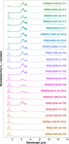 |
Fig. 1 Spectral sample of 22 T and Y dwarfs originally published in Beiler et al. (2024a). All spectra have been normalized at their maximum flux value and offset by a constant. |
Retrieval parameters and prior distributions for the free chemistry approach used in the cloud-free and non-gray cloud models.
3.2 Machine learning framework
In addition to retrievals within a Bayesian framework, we applied atmospheric retrievals using the random forest supervised machine learning algorithm (Ho 1998; Breiman 2001), implemented through the HELA code (Márquez-Neila et al. 2018). The HELA code combines the use of decision trees (e.g., Breiman et al. 1984) with bootstrapping techniques (e.g., Efron & Tibshirani 1994) and can be applied to both discrete and continuous training sets.
A key advantage of random forest retrievals is their computational efficiency and ability to quantify feature importance, therefore enabling ranking of the relative influence of individual spectral data points (features) in constraining specific model parameters. This interpretability has made random forests particularly appealing for atmospheric retrievals in studies of exoplanets and brown dwarfs (Márquez-Neila et al. 2018; Oreshenko et al. 2020; Fisher et al. 2020; Guzmán-Mesa et al. 2020; Fisher & Heng 2022; Lueber et al. 2023, 2024).
The random forest method HELA uses precalculated grids of model spectra as individual training data within the approximate Bayesian computation framework (Sisson et al. 2018). In our approach, all model spectra, which are described in the next section, were binned to the overlapping wavelength ranges of the spectra by Beiler et al. (2024a), which were obtained with JWST. The NIRSpec PRISM and MIRI LRS spectra cover the ~1-12 μm wavelength range at λ∕∆λ ≈ 100. For each random forest spectral fitting, 3000 regression trees were utilized, and each tree was allowed to grow without a limit on depth. The trees were pruned only when additional splits resulted in a variance reduction smaller than 0.01. Furthermore, the maximum number of features allowed for splitting at each node was restricted to the square root of the total number of spectral data points utilized.
The performance of a trained model is typically assessed using real versus predicted (RvP) plots. These comparisons are quantitatively evaluated using the coefficient of determination,
 (3)
(3)
where Sres is the sum of squared residuals between real (yi) and predicted (fi) values,
 (4)
(4)
and Stot represents the total variance of the real values,
 (5)
(5)
The R2 value indicates how well the model generalizes to unseen data: R2 = 1 indicates perfect predictions, R2 = 0 suggests no correlation, and R2 < 0 indicates predictions that are worse than random chance.
Here, we briefly summarize the model grids used in this work. We reduced the number of models by constraining them to ranges 200 K ≤ Teff ≤ 800 K, 3.0 ≤ log g ≤ 6.0 (in units of cm/s2), −1.0 ≤ [M/H] ≤ +1.0, and 0.5 ≤ C/O ≤ 1.5. These constraints are, in addition to the parameter limits set in the original model grids, described below. The exact parameter ranges are listed in Table 3.
HELIOS. The open-source radiative transfer code HELIOS (Malik et al. 2017, 2019) utilizes an improved two-stream method (Heng & Kitzmann 2017; Heng et al. 2018) that incorporates non-isotropic scattering and convective adjustment. The equilibrium gas-phase chemistry was computed with the original version of the open-source FASTCHEM equilibrium chemistry code5 (Stock et al. 2018, 2022), which did not include condensation (Kitzmann et al. 2024). Within the cloud-free HELIOS atmosphere grid, the removal of gas-phase species due to condensation was approximated using stability curves of various condensates (see Appendix B in Malik et al. 2017 for details). The elemental abundances for the chemistry calculations are based on those of the Sun’s photosphere from the compilation by Asplund et al. (2009).
Sonora Bobcat. The atmospheric grid by Marley et al. (2021) known as Sonora Bobcat consists of cloud-free models developed for radiative-convective equilibrium atmospheres using a layer-by-layer convective adjustment method. This grid enables solutions with distinct convective zones. Rainout chemistry incorporates condensation from the gas phase, as described by Lodders & Fegley (2006), but does not consider explicit cloud opacity. The models adopt the k-distribution approach for calculating wavelength-dependent gas absorption (Goody et al. 1989), utilizing updated opacities and equilibrium constants for gas-phase chemistry (for additional details, see Marley et al. 2021).
Sonora Elf Owl. The Sonora Elf Owl models (Mukherjee et al. 2024) are the latest additions to the Sonora series, which includes the Bobcat (Marley et al. 2021), Cholla (Karalidi et al. 2021), and Diamondback (Morley et al. 2024) models. The Cholla models introduced self-consistent disequilibrium chemistry, though they are limited to solar composition, while the Diamondback models incorporate the effects of clouds and metallicity on atmospheric structure. The Elf Owl models offer a further advancement with a self-consistent, cloud-free 1D radiative-convective equilibrium framework and include mixing-induced disequilibrium chemistry beyond solar composition and account for non-solar C/O ratios. The Elf Owl model features additional free parameters such as the vertical eddy diffusion coefficient, κzz, and explores broader parameter spaces compared to previous versions. We applied the updated version 2 model with corrected disequilibrium CO2 abundance and PH3 contributions removed (see Beiler et al. 2024b and Wogan et al. 2025).
Lacy & Burrows. The atmospheric model grid by Lacy & Burrows (2023) consists of 1D radiative-convective equilibrium models produced with coolTLUSTY for plane-parallel atmospheres. Chemical abundances are calculated assuming either equilibrium or non-equilibrium chemistry driven by vertical mixing, following Hubeny & Burrows (2007), and encompass processes such as condensation and rainout. For effective temperatures below 400 K, the models incorporate water clouds using a parameterized, spatially uniform prescription.
ATMO2020++ without PH3. The ATMO2020++ grid without PH3 (Leggett & Tremblin 2025) is an updated version of the original ATMO2020 models6 (Phillips et al. 2020) incorporating empirical modifications to better reproduce the observed spectra of late-T and Y dwarfs. In particular, the temperature gradient in convective regions has been reduced - by adopting a lower effective adiabatic index - to create cooler deep atmospheres, where the near-infrared flux originates, and warmer upper layers, which emit in the mid-infrared. Although this modification is not derived from first principles, it is physically motivated and may reflect processes such as the inhibition of convection by condensate formation or rapid rotation, though these explanations remain unproven (see Leggett & Tremblin 2025 for a discussion). The model is tailored for solar metallicity and metalpoor atmospheres. Disequilibrium chemistry is utilized with a vertical eddy diffusion coefficient, κzz, which is set at κzz = 105 cm2∕s for log g = 5.0 and is scaled by 10(2∙(5−log g)) for other surface gravities. The scaling κzz ∝ g−2 reflects the change in atmospheric scale height with gravity and its impact on vertical mixing efficiency and chemical disequilibrium.
Parameter ranges for spectral model grids.
3.3 Feature importance analysis of JWST NIRSpec+MIRI modes: Case study for the Y1 dwarf WISEPAJ1541-22
To investigate feature importance using the random forest approach, we generated a model grid of 100 000 synthetic spectra by using the forward model of BEAR. Most parameters were sampled from uniform distributions, while volume mixing ratios followed log-uniform distributions. For the current study, no noise was considered in the creation of the grid.
The grid was constructed using the following prior ranges: surface gravity log gbetween 2.0 and 5.5, scaling factor f from 0.2 to 2, and distance d specific to the considered object, sampled from a range of uncertainties around its known value in parsecs (5.99 ± 0.07 pc, for the Y1 dwarf WISEPAJ1541-22). The molecular log abundances were drawn from a uniform distribution between 10−12 and 10−2 for the ten key molecules: H2O, CO, CO2, H2S, K, Na, SO2, CH4, PH3, and NH3.
The temperature structure was defined by a base temperature, T0, at the bottom of the modeled atmosphere sampled between 500 and 3000 K; an adiabatic index γ between 1.0 and 2.0; a radiative-convective boundary 102 ≤ RCB ≤ 1.0 bar; and subsequent layers above set by applying factors b1 to b4 that scale the temperature at each level between 0.1 and 0.95 of the layer below. Cloud top pressures, pt, and (vertical) gray optical depths, τc, were sampled within the ranges of 10−3 to 102 bar and −10 to 20, respectively.
This grid enabled us to train a random forest model, which was evaluated using RvP assessments, quantified by the coefficient of determination R2 (see Fig. A.1). The temperature at the base of the atmosphere, T0, demonstrated high self-consistency, while the predictability diminishes with each additional temperature-pressure profile coefficient, bi. This decline is due to the emission spectrum becoming increasingly insensitive to temperature variations in the upper atmosphere.
At higher abundances, most chemical species show strong predictability. Exceptions include species such as sodium and potassium, which lack the broad absorption bands typical of many molecules. At lower abundances, detection becomes more challenging, leading to reduced sensitivity in the RvP plots.
The contribution of different wavelength regions to parameter inference was analyzed using the feature importance plots shown in Fig. 2. These highlight how specific spectral features relate to physical and chemical processes, such as pressure broadening, vibrational transitions, and disequilibrium chemistry.
The surface gravity log g exhibits strong spectral importance, particularly at shorter wavelengths, due to the broad pressure-broadened wings of alkali metal resonance lines. It also shows a distinct peak near 2.0 μm, likely associated with collision-induced H2 absorption (Linsky 1969; Burgasser et al. 2002). Because collision-induced absorption arises from collisions between gas-phase molecules, it is highly pressuresensitive. While the feature importance analysis suggests that log g contributes mainly at shorter wavelengths, this does not imply that it has no impact at longer wavelengths. In fact, gravity significantly affects CO and CO2 absorption around 5 μm, as shown in Lacy & Burrows (2023) and Leggett & Tremblin (2025). The flux scaling factor f, acting as a proxy for planetary radius (see Sect. 3.1), shows peaks in the water absorption bands between 1.8 and 3.0 μm and in the mid-infrared beyond 11 μm.
Water vapor (H2O) dominates the opacity across many wavelengths, with strong contributions at 1.4 μm and 2.7 μm as well as broader importance between 5.0 and 7.0 μm, underscoring its central role in shaping both continuum and absorption features. Carbon-bearing species such as CO and CO2 peak at 4.6 μm and 4.2 μm, respectively, consistent with their presence in warmer or vertically mixed atmospheres.
Alkali metals Na and K are influential in the 0.7-1.0 μm range due to their broad absorption profiles, which also help constrain gravity. Sulfur-bearing species such as H2S show slight contributions between 2.5-4.0 μm, though they are typically masked by stronger absorbers. Sulfur dioxide (SO2), which is usually absent under equilibrium conditions, exhibits midinfrared importance near 7.3-8.7 μm, where it could possibly indicate disequilibrium processes.
Methane (CH4), a key absorber in cooler atmospheres, is prominent around 3.3 μm, reflecting its increasing opacity at lower temperatures. Ammonia (NH3) contributes notably between 10 and 11 μm in the cooler atmospheres of late-T and Y dwarfs. Phosphine (PH3) displays localized importance near 4.3 μm, with minor features across the spectrum, which is consistent with expectations for reducing atmospheric conditions.
The base temperature T0 is primarily constrained by features below 2.0 μm and is closely linked to the surface gravity due to its effect on the pressure-temperature profile. The thermal structure parameters b1 through b4 exhibit a progressively weaker spectral influence. The parameters b1 and b2 that describe the deeper atmospheric temperature gradient still show some distinct spectral feature importance peaks, indicating sensitivity at certain wavelengths. The parameters b3 to b4, on the other hand, describe the temperature-pressure profile in the upper layers. Here, however, the spectrum is almost unaffected by the form of the profile. Consequently, no distinct peaks are visible in the feature importance plots. We note that the feature importance is a normalized measure for each parameter, and hence absolute values cannot be directly compared across different parameters.
Only limited insights can be gained from the feature importance of the adiabatic index (γ), the RCB, and the cloud model parameters such as cloud-top pressure (pt) and gray optical depth (τc). These parameters exhibit a slightly decreasing importance from the near- to mid-infrared, but they show a localized significance around 5 μm. We speculate that the increased importance of the data at around 5 microns is likely due to the region’s sensitivity to cloud properties affecting emergent flux.
By interpreting feature importance plots, we effectively reverse-engineer the spectroscopic fingerprints that encode the model parameters. This data-driven approach provides valuable insights into opacity physics, thermal structure, and chemical composition. However, this information does not help retrieve precise parameters for individual objects. Instead it leads to better understanding of which spectral features are most informative, therefore guiding future retrieval efforts. It also allows us to understand how different model grids emphasize each of these aspects differently across wavelength.
4 Results and discussion
The primary aim of this study is to revisit and adapt longstanding research questions from the initial investigation by Lueber et al. (2022), specifically tailoring them to explore the unique characteristics of late-T and Y dwarfs. While previous work has provided insights, key questions have remained unresolved or require reevaluation within the context of the colder and less luminous objects analyzed here. With this study, we seek to bridge that gap in order to advance our understanding of these enigmatic ultra-cool brown dwarfs.
4.1 Retrieval of the Y1 dwarf WISEPAJ1541-22
Before we present the overall trends in the retrieved properties across the T-Y sequence as a function of the effective temperature, we first discuss the results for the Y1 dwarf WISEPAJ1541-22 in more detail. The posterior distributions for this object are shown in Fig. 3, while the posterior median spectra and the comparison to the observed spectrum are depicted in Fig. 4. To account for underestimated uncertainties or unmodeled systematics, we considered additional variance using  (see Kitzmann et al. 2020). The retrieved error inflation parameter
  corresponds to a flux level of
  = (1.11 ± 0.05) ∙ 10−18 W m−2μm−1, which is comparable to the largest reported uncertainty for WISEPAJ1541-22. This results in an overall increase in uncertainty by a factor of approximately two.
For this object we find a strong preference for a gray cloud over a cloud-free model by performing Bayesian model comparison (ln Bij = 11.12; see Table 4). Additionally, we find high abundances of both CO and CO2 compared to equilibrium chemistry calculations. The posterior distributions in Fig. 3 illustrate degenerate joint posteriors among the retrieved molecular abundances of H2O, CO, CO2, CH4, and NH3 as well as their association with the retrieved surface gravity log g. Notably, the retrieved thermal profile indicates that the cloud top is located at  bar (
bar ( bar). This positioning lies near the anticipated condensation temperature of water vapor at ~300 K but remains too warm for condensation to occur at this pressure level. Water clouds, if present, would form at higher altitudes where the temperature decreases further. Nonetheless, the optical depth of the cloud layer (
 ) supports the existence of an optically dense and vertically extended cloud layer, in alignment with the predicted onset of water cloud formation for late-T and Y dwarfs. Furthermore, the constraint of the adiabatic index γ of
  is consistent with a mixture of molecular hydrogen and helium.
The simultaneous presence of CO and CH4 at such low effective temperatures (Teff =  K) likely reflects vertical mixing and chemical quenching within the deep atmosphere. Collectively, these findings firmly position WISEPAJ1541-22 within the transition regime where clouds constitute a significant atmospheric component, thereby providing empirical support for theoretical predictions concerning the evolution of condensate clouds within Y dwarf atmospheres.
Based on the retrieved abundances, we derived an overall metallicity of [M/H] = 0.22 ± 0.03 by summing the elemental abundances relative to hydrogen and normalizing to their solar values. The derived metallicity corresponds to approximately 1.7 times the solar elemental abundance (using solar values from Asplund et al. 2009: C/H = 2.69 ∙ 10−4, N/H = 6.76 ∙ 10−5, O/H = 4.90 ∙ 10−4). However, this enrichment is not uniform across all elements. Carbon, for instance, is enriched by a factor of 2.7, and oxygen by a factor of 1.3, while nitrogen shows a mild depletion of ~0.3 with respect to its solar value. We note, however, that the latter elemental abundance is based on ammonia alone. Nitrogen might still be present in other molecules, such as molecular nitrogen (N2), that have no distinct spectral features in the wavelength range of the observations used here. The resulting carbon-to-oxygen (C/O) ratio is 1.12 ± 0.14, corresponding to (C/O)/(C/O)⊙ = 2.0 ± 0.4, relative to the solar value of C/O⊙ = 0.55 ± 0.09 (Asplund et al. 2009).
The prior distribution of the C/O ratio, derived from combinations of molecular gas abundance priors, exhibits a characteristic double-peaked structure, with maxima at (C/O)/(C/O)⊙ ≈ 1 and (C/O)/(C/O)⊙ ≈ 1.8, regardless of whether the priors of molecules are log-uniform or broad Gaussian (Line et al. 2013). The former is caused by the abundance of CO2, which would result in a solar-like C/O ratio of 0.5, while the latter is determined by CO. Consequently, the prior distribution for the C/O ratio is directly affected by the choice of molecules included in a retrieval.
A comparison of this analytically constructed prior to the posterior distribution derived from the constrained molecular abundances in the atmosphere of WISEPAJ1541-22 is shown in Fig. 5. A clear divergence can be seen: The posterior does not exhibit the double-peaked structure characteristic of the prior.
This indicates that the data provide meaningful constraints on the C/O ratio. In particular, the absence of the prior’s double peaks in the posterior suggests that JWST observations are sufficient to break prior degeneracies and extract genuine information about the C/O ratio. This result underscores the power of JWST in constraining elemental abundance ratios in brown dwarf atmospheres.
Using a grid-fit retrieval with the ATMO2020++ atmosphere model grid, Tu et al. (2024) derived a much lower metallicity of [M/H] = −0.21 ± 0.01. It is important to note, however, that the metallicity values derived from retrieval calculations assume that all major carriers of each element are adequately constrained. Species with limited spectral signatures, such as molecular nitrogen, may not significantly contribute to the observed spectrum and could therefore be absent from the metallicity estimates. As a result, our derived N/H value should be interpreted as a lower limit.
The apparent enrichment of carbon relative to oxygen may partly result from condensation processes. In the deeper layers of the atmosphere, some oxygen is sequestered into oxygen-bearing condensates, such as forsterite (Mg2SiO4). As a result, the gasphase C/O ratio may still not accurately reflect the atmosphere’s bulk composition.
To assess the consistency of our results from a chemical perspective, we performed additional calculations using the FASTCHEM chemistry code (Stock et al. 2018, 2022). FASTCHEM is a chemical equilibrium model that includes condensate formation (Kitzmann et al. 2024) and incorporates the commonly used rainout approximation, which is particularly relevant for brown dwarf atmospheres. For this analysis, we used the temperature-pressure profile and elemental abundances for C, O, and N, which were obtained from the retrieval results to compute the gas-phase chemical composition and the potential formation of condensates as a function of pressure. The results are shown in Fig. 6. For these calculations, we employed an expanded set of chemical elements, gas-phase species, and condensates recently added to FASTCHEM (Kitzmann et al., in prep.).
The gas-phase mixing ratios for H2O, CH4, and NH3 predicted by FASTCHEM are consistent with the retrieved abundances. These species also appear to exhibit nearly constant mixing ratios (i.e., isoprofiles), supporting the common retrieval assumption of uniform vertical abundances. In contrast, the equilibrium abundances of CO2 and CO are significantly lower than the retrieved values, suggesting the influence of vertical mixing. As shown in Fig. 6, this mixing likely originates from pressure levels around ~102 bar, where the retrieved abundances intersect the chemical equilibrium curves.
The bottom panel of Fig. 6 displays the stable condensate species predicted by FastChem using the rainout approach. Three commonly considered condensates, potassium chloride (KCl), zinc sulfide (ZnS), and sodium chloride (NaCl), appear to form too deep in the atmosphere compared to the retrieved cloud pressure of approximately 0.5 bar. Notably, H2O and NaS2 are not predicted to be present by FastChem.
Interestingly, two species predicted to be stable near 0.5 bar are arsenic(II) sulfide (As2S2(s,l)) and ammonium bromide (NH4Br(s)). Whether these species are sufficiently abundant to form optically thick cloud layers remains uncertain. A definitive assessment would require detailed cloud-formation modeling, which is beyond the scope of this study.
The atmospheric retrieval supports the presence of an optically thick cloud layer. However, though chemical equilibrium calculations point to plausible condensate candidates, no further definitive conclusion may be drawn.
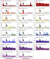 |
Fig. 2 Feature importance across wavelengths for all parameters included in our generated model grid for the case study of the Y1 dwarf WISEPAJ1541-22 as well as their joint retrieval. The significance of a feature is quantified by the normalized decrease in variance it generates throughout the training process. Specifically, it denotes the total reduction in variance achieved whenever that feature is employed for partitioning nodes in a decision tree within the ensemble. For visual guidance, the rescaled spectrum of WISEPAJ1541-22 is overlaid as solid black lines. |
 |
Fig. 3 Joint posterior distributions from the free-chemistry retrieval analyses of the case study Y1 dwarf WISEPAJ1541-22 using a gray cloud model. The vertical dashed lines within the histograms indicate the median parameter values and their 1σ uncertainties. Accompanying the montage of joint posterior distributions is the retrieved median temperature-pressure profile along with its associated 1σ uncertainties. The adiabatic profile (dashed black line) is indicated for comparison. |
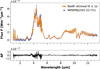 |
Fig. 4 Posterior retrieval median fit, F (orange line), and residuals, ∆F (black line), associated with the free-chemistry retrieval analyses of the case study Y1 dwarf WISEPAJ1541-22 using a gray cloud model. The retrieved error inflation is represented by a horizontal gray bar. The JWST NIRSpec and MIRI data are shown as blue dots with associated uncertainties. |
Bayesian statistics for the retrieval analysis of the curated set of brown dwarfs.
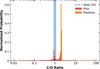 |
Fig. 5 Normalized carbon-to-oxygen (C/O) ratio probabilities expressed relative to the solar value of 0.5 5 ± 0.09 (Asplund et al. 2009) for the case study Y1 dwarf WISEPAJ1541-22. Prior (red) and posterior (orange) probability distributions were derived from combinations of molecular gas abundance distributions. The solar value is indicated with a dashed blue line and shaded region. |
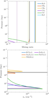 |
Fig. 6 Chemical composition for Y1 dwarf WISEPAJ1541-22 calculated with FastChem. The upper panel shows the volume mixing ratios of major gas-phase species. Retrieved abundances from the BeAR retrieval and their 1σ confidence intervals are depicted by the shaded areas. Stable condensates are shown in the lower panel. Their number densities, nc, refer to the effective molecule number contained in the condensed phase and do not correspond to an actual cloud particle number density. The cloud top position and its 1σ confidence interval constrained by the retrieval calculations ( |


4.2 The role of clouds in modeling the spectra of late-T and Y dwarfs
Clouds have long been considered essential for accurately modeling the spectra of late-T and Y dwarfs, particularly because they help replicate the spectral reddening observed in these ultra-cool objects. The work by Morley et al. (2012, 2014) emphasizes this point, demonstrating that water and sulfide clouds, which become optically significant at effective temperatures below 350-375 K, can align model spectra more closely with observational data.
However, findings by Tremblin et al. (2015) challenge this necessity, presenting a cloud-free alternative that successfully reproduces the spectra of Y dwarfs when accounting for factors such as vertical mixing and NH3 quenching. Tremblin et al. (2015) suggest that modifying the atmospheric temperature gradient to incorporate fingering convection - a process driven by condensation and subsequent chemical quenching - can explain the reddening previously attributed to clouds.
Leggett et al. (2017) examined the atmospheric properties of Y-type brown dwarfs and found that non-equilibrium cloud-free models accurately replicate the near-infrared spectra and mid-infrared photometry of warmer Y dwarfs with effective temperatures between 425 K and 450 K. While Y dwarfs are often modeled with cloud-free atmospheres due to their low temperatures, Leggett et al. (2017) proposed that thin cloud layers composed of sulfides and other condensates might still influence the spectra of even colder Y dwarfs, particularly in the near-infrared range. Recently, Lacy & Burrows (2023) developed a set of self-consistent model atmospheres for Y dwarfs and highlighted that disequilibrium in CH4-CO and NH3-N2 chemistry, along with the presence of water clouds, could improve, although still not fully resolve, the agreement between models and observations of Y dwarfs.
Knowing that Y dwarfs are rapid rotators (Hsu et al. 2021), rotational dynamics are expected to substantially impact atmospheric energy transport, as recent atmospheric circulation models of brown dwarfs and exoplanets have demonstrated (Tan & Showman 2021). Recent enhancements to general circulation model simulations have included the integration of consistent chemical equilibrium, advanced cloud microphysics, and fully coupled three-dimensional radiative transfer, enabling a more accurate representation of the atmospheric conditions of the coldest brown dwarfs (Lee & Ohno 2025).
These findings imply that turbulence, vertical mixing, and disequilibrium chemistry dominate the shaping of the spectra of late-T and Y dwarfs. The presence or absence of water clouds is still under active debate. In the context of our Bayesian model comparison analysis, cloud-free models are preferred for the hottest objects of the curated sample (T6-T8), while later type objects vary in their preference for gray cloud and cloud-free models, sometimes providing equally good fits to the data (Table 4). Non-gray models were never preferred by the data in the atmospheric retrieval analysis of our curated set of 22 late-T and Y dwarfs. However, strong indications can be found for the presence of vertical mixing and disequilibrium chemistry. While our retrieval framework captures the effects of these processes, it does not rule out alternative explanations such as fingering convection proposed by Tremblin et al. (2015), which may produce similar observational signatures.
 |
Fig. 7 Comparison of retrieved posterior outcomes for effective temperature (top), surface gravity (middle), and radii (bottom) from our suite of brown dwarf retrievals across the T-Y sequence. The brown dwarfs are ordered with respect to their spectral class, from T6 to Y1 (see Table 1 for details). For each object within the curated sample, all permutations of the theoretical grid models, which were used for training the HELA random forest routine, are shown as well as the posterior parameters retrieved by using the nested sampling BeAR framework. For each posterior, the 1σ uncertainties are shown, but they are too small to be visible for the BeAR posteriors. Gray bars in the top panel indicate the effective temperature values determined by Beiler et al. (2024a) using integrated luminosities and radii from evolutionary models (see their Table 4). |
4.3 Trends in the retrieved surface gravity, effective temperature, and radii across the T-Y transition
In this section, we examine trends in the retrieved physical properties of brown dwarfs across the T-Y spectral sequence. Key parameters, including effective temperature (Teff), surface gravity (log g), and radius (R), are presented in Fig. 7 for the complete sample analyzed in this study. We compared results from atmospheric retrievals using the Bayesian atmospheric retrieval code BeAR with those obtained from random forest machine learning models trained on various atmospheric grids, as introduced in Sect. 3.2. The posterior spectral fits and all retrieved temperature-pressure profiles are shown in Figs. A.2 and A.3.
Across the T-Y transition, the retrieved values align well with predictions from brown dwarf evolutionary models (e.g., Filippazzo et al. 2015; Kirkpatrick et al. 2021; Marley et al. 2021). As shown in Fig. 7, effective temperatures decrease from ~ 1000 K in late-T dwarfs to ~400 K in Y dwarfs (Cushing et al. 2011; Leggett et al. 2017). As brown dwarfs cool over timescales of gigayears (Gyr), their mass, radius, and effective temperature are intrinsically linked through evolutionary cooling tracks (Marley et al. 2021). While evolutionary models predict a modest increase in surface gravity as a result of long-term contraction, the associated change in radius is small, and no clear trend in log g is observed in our retrieval outcomes. Notably, retrievals often yield broader log g distributions for Y dwarfs (Zalesky et al. 2022), likely due to degeneracies between temperature, gravity, and cloud opacity, compounded by limited spectral resolution in observations of these faint objects. Additionally, comparing retrieved radii with model predictions, which suggest nearly constant values between 0.8 and 1.2Rjup, is complicated by uncertainties in object age and cloud structure (Burrows et al. 2011). For a local sample of cool and faint brown dwarfs, ages of a few gigayears—comparable to the Sun—are expected and consistent with recent population studies (Best et al. 2024). For example, at an age of ~4 Gyr, evolutionary models predict that a 750 K T dwarf has log g ≈ 5.1 and R ≈ 0.088 Rjup, while a 400 K Y dwarf has log g ≈ 4.6 and R ≈ 0.101 Rjup, which is broadly consistent with the trends shown in Fig. 7. In some cases, the retrieved radii are anomalously large, as observed for the Y1 dwarf WISEJ0535-75. These discrepancies may indicate unresolved binarity, a younger age, or systematic errors in distance estimates or atmospheric modeling. However, we generally do not face the well-known radius problem, where retrieved radii tend to be unphysically small.
The retrieval approaches we used, nested sampling and random forest, produced broadly consistent results. Discrepancies in retrieved temperatures were found primarily for the hottest objects in the sample, including the T6 dwarfs SDSSJ1624+00 and WISEJ1501-40 and the T6.5 dwarf SDSSpJ1346-00. These differences are attributed to the upper temperature limit (800 K) of the atmospheric model grid used in the machine learning model. Moreover, the random forest method generally produced more conservative estimates, characterized by larger uncertainties. This behavior likely results from limitations in the size and resolution of the training grid (see, e.g., Lueber et al. 2023).
Comparisons with previous studies (Beiler et al. 2024a; Tu et al. 2024) show good agreement in effective temperature estimates, while greater variability is seen in retrieved surface gravities, which are inherently more model-dependent given the strong degeneracy between surface gravity and metallicity when fitting spectra of late-T and Y dwarfs. One notable exception is the Y1 dwarf CWISEPJ1047+54. Tu et al. (2024) report a remarkably low surface gravity of log g = 2.50 ± 0.01 from their ATM02020++ grid fit, whereas our BEAR retrieval yields a significantly higher value of log g = 5.34 ± 0.08. Tu et al. (2024) caution that their posterior converged at the edge of the model grid and should be interpreted with care. This sensitivity to model assumptions is further illustrated by the large differences in surface gravity and metallicity found by Tu et al. (2024) when comparing ATM02020++ and Sonora Elf Owl models, underscoring the impact of model-dependent degeneracies. While the random forest trained on a variety of grids that also predict smaller log g values for this object than BEAR, these values are still considerably higher than the estimate by Tu et al. (2024). We note that log g ≳ 5 for Y dwarfs would imply implausibly old ages greater than 15 Gyr according to evolutionary models, likely indicating residual degeneracies in the models rather than physical constraints. In contrast, effective temperature estimates for this object differ by only ~50K, with Tu et al. (2024) reporting Teff = 381.0 ± 0.2 K and our BEAR retrieval yielding Teff = 430 ± 6 K when using a gray cloud model. Despite this discrepancy, the overall consistency across the retrieval techniques underscores the robustness of the inferred atmospheric parameters within the bounds of current model limitations.
4.4 Insights into the atmospheric chemistry of late-T and Y dwarfs
The atmospheres of late-T and Y dwarfs exhibit complex chemical interactions influenced by disequilibrium processes and vertical mixing as well as by condensate rainout, all of which have been established by early observational and theoretical studies (e.g., Noll et al. 1997; Saumon et al. 2000; Leggett et al. 2007; Geballe et al. 2009; Lodders 1999; Visscher et al. 2006, 2010; Morley et al. 2012). These mechanisms significantly affect the abundances of key molecules such as CO, CH4, CO2, NH3, and PH3. Zahnle & Marley (2014) demonstrated that vertical mixing enhances CO abundances beyond equilibrium predictions, even in the colder atmospheres of late-T and Y dwarfs, where CH4 would otherwise dominate. This disequilibrium effect is particularly pronounced in low-gravity objects, as it transports CO from deeper, hotter regions into the observable atmosphere, thereby challenging traditional equilibrium-based models. It is further enhanced at higher metallicities, which increases vertical mixing (Zahnle & Marley 2014).
Observational studies support these theoretical predictions. Miles et al. (2020) detected CO in late-T and Y dwarfs at levels inconsistent with equilibrium chemistry. Similarly, Hubeny & Burrows (2007) showed that vertical mixing alters both the thermal structure and spectral features, highlighting the importance of including disequilibrium chemistry in atmospheric modeling.
Beiler et al. (2024b) examined discrepancies in the predicted abundances of PH3 and CO2, noting that existing models often underestimate CO2 while overestimating PH3 in cool atmospheres. This suggests an incomplete understanding of phosphorus chemistry in late-T and Y dwarfs. Morley et al. (2014) further predicted that PH3, although difficult to detect under equilibrium conditions, could become more abundant through disequilibrium processes, leading to a prominent mid-infrared spectral feature near 4.3 μm in Y dwarfs with Teff ~ 450 K.
Our retrieval analysis provides additional evidence of chemical disequilibrium, as illustrated in Fig. 8 and summarized in Tables B.1-B.4. Notably, CH4 and CO are retrieved simultaneously, consistent with the scenario described by Zahnle & Marley (2014), in which vertical mixing transports CO into the upper atmosphere. Furthermore, our results confirm the findings of Beiler et al. (2024b): PH3 is absent or weakly present in the observed atmospheres, while CO2 appears in higher-than-expected concentrations in several objects compared to equilibrium chemistry calculations. In this low-temperature regime, CO and CO2 abundances are highly sensitive to the location of the chemical quench level such that small variations in vertical mixing or thermal structure can lead to significant changes in the retrieved volume mixing ratios across the sample.
Trends in the retrieved abundances of H2O, CH4, and NH3 show an anticipated decline with increasing effective temperature (Teff), in agreement with the results of Zalesky et al. (2019, 2022). In particular, NH3 in the near-infrared is only detectable in Y dwarfs, reinforcing its role as a spectral signature of the Y dwarf class.
A clear depletion trend is also observed for potassium, decreasing from the hotter late-T dwarfs to the cooler Y dwarfs. This trend aligns with predictions from the Sonora Elf Owl model grid (Mukherjee et al. 2024) and is driven by rainout chemistry. Around 1300 K, aluminum and silicate condensates begin to form, depleting the available elemental reservoirs. Subsequent additional elements are depleted as well, including sodium and potassium near 700 K. There they condense into Na2S(s) and KCl(s), respectively (Zalesky et al. 2022).
5 Summary and conclusions
In this study, we have performed a retrieval analysis on a curated sample of 22 late-T and Y dwarfs originally observed by Beiler et al. (2024a) using the NIRSpec and MIRI instruments aboard the JWST. Our main findings are summarized as follows:
Clouds play a critical role in modeling the spectra of late-T and Y dwarfs, with their impact modulated by vertical mixing and disequilibrium chemistry. Bayesian model comparison indicates that cloud-free models are generally favored for the hottest objects in the sample (T6-T8). In contrast, later-type dwarfs show varying preferences, with both gray cloud and cloud-free models yielding comparable fits. Several objects exhibit clear signatures of disequilibrium chemistry. Notably, the Y1 dwarf WISEPAJ1541-22 favors a gray cloud model and shows elevated abundances of both CO and CH4;
The retrieved physical parameters across the T-Y spectral transition are consistent with predictions from evolutionary models. Specifically, effective temperatures decrease across the sample, while radii remain within the expected range of 0.8-1.2RJup. The results are generally consistent within uncertainties between the Bayesian nested-sampling atmospheric retrieval and the supervised machine learning random forest approach. We did not encounter the well-known radius problem in atmospheric retrievals, where retrieved radii are often constrained to be unphysically small;
The retrievals from nested sampling and random forest methods show strong overall agreement. However, the random forest results tend to be more conservative, with broader uncertainties-an outcome primarily reflecting the method’s intrinsic tendency to average over parameter space. Additionally, limitations in grid resolution and spacing may further contribute to this broadening;
The atmospheres of late-T and Y dwarfs show evidence of chemical disequilibrium, particularly due to vertical mixing. Both CH4 and CO are retrieved, with CO likely transported from deeper atmospheric layers. As physically expected, retrieved abundances of H2O, CH4, and NH3 decrease with increasing effective temperature, which is consistent with trends reported by Zalesky et al. (2019, 2022).
 |
Fig. 8 Posterior BeAR retrieval values for molecular log-volume mixing ratios (log VMR) of H2O, CH4, NH3, K, CO2, and CO plotted against the retrieved effective temperature (Teff; shown in red). For visual comparison, modeled volume mixing ratios from the Sonora Elf Owl model grid (Mukherjee et al. 2024) are overlaid for a surface gravity of log g = 5.0 (cgs units) and a vertical eddy diffusion coefficient of log κzz = 8.0 with varying metallicities ([M/H]) and carbon-to-oxygen (C/O) ratios relative to solar. |
Acknowledgements
This work is based [in part] on observations made with the NASA/ESA/CSA James Webb Space Telescope. The data were obtained from the Mikulski Archive for Space Telescopes at the Space Telescope Science Institute, which is operated by the Association of Universities for Research in Astronomy, Inc., under NASA contract NAS 5-03127 for JWST. The specific observations analyzed can be accessed via https://dx.doi.org/10.17909/dwnb-jv28. These observations are associated with program #2302. We acknowledge partial financial support from the Swiss National Science Foundation (via grant no. 192022 awarded to K.H.), the European Research Council (ERC) Geoastronomy Synergy Grant (via grant no. 101166936 awarded to K.H.), as well as administrative support from the Center for Space and Habitability (CSH). D.K. acknowledges the support from the Swiss National Science Foundation under the grant 200021-231596. We also like to thank Adam Burgasser for his valuable input.
References
- Abel, M., Frommhold, L., Li, X., & Hunt, K. L. C. 2011, J. Phys. Chem. A, 115, 6805 [NASA ADS] [CrossRef] [Google Scholar]
- Abel, M., Frommhold, L., Li, X., & Hunt, K. L. C. 2012, J. Chem. Phys., 136, 044319 [NASA ADS] [CrossRef] [Google Scholar]
- Allard, N. F., Spiegelman, F., & Kielkopf, J. F. 2016, A&A, 589, A21 [NASA ADS] [CrossRef] [EDP Sciences] [Google Scholar]
- Allard, N. F., Spiegelman, F., Leininger, T., & Molliere, P. 2019, A&A, 628, A120 [NASA ADS] [CrossRef] [EDP Sciences] [Google Scholar]
- Asplund, M., Grevesse, N., Sauval, A. J., & Scott, P. 2009, ARA&A, 47, 481 [CrossRef] [Google Scholar]
- Azzam, A. A. A., Tennyson, J., Yurchenko, S. N., & Naumenko, O. V. 2016, MNRAS, 460, 4063 [NASA ADS] [CrossRef] [Google Scholar]
- Barber, R. J., Tennyson, J., Harris, G. J., & Tolchenov, R. N. 2006, MNRAS, 368, 1087 [Google Scholar]
- Beiler, S. A., Cushing, M. C., Kirkpatrick, J. D., et al. 2024a, ApJ, 973, 107 [NASA ADS] [CrossRef] [Google Scholar]
- Beiler, S. A., Mukherjee, S., Cushing, M. C., et al. 2024b, ApJ, 973, 60 [Google Scholar]
- Best, W. M. J., Liu, M. C., Magnier, E. A., & Dupuy, T. J. 2020, AJ, 159, 257 [Google Scholar]
- Best, W. M. J., Sanghi, A., Liu, M. C., Magnier, E. A., & Dupuy, T. J. 2024, ApJ, 967, 115 [NASA ADS] [CrossRef] [Google Scholar]
- Breiman, L. 2001, Mach. Learn., 45, 5 [Google Scholar]
- Breiman, L., Friedman, J., Stone, C., & Olshen, R. 1984, Classification and Regression Trees (Taylor & Francis) [Google Scholar]
- Burgasser, A. J. 2014, in Astronomical Society of India Conference Series, 11, Astronomical Society of India Conference Series, 7 [Google Scholar]
- Burgasser, A. J., Kirkpatrick, J. D., Brown, M. E., et al. 2002, ApJ, 564, 421 [NASA ADS] [CrossRef] [Google Scholar]
- Burgasser, A. J., Geballe, T. R., Leggett, S. K., Kirkpatrick, J. D., & Golimowski, D. A. 2006, ApJ, 637, 1067 [Google Scholar]
- Burningham, B., Cardoso, C. V., Smith, L., et al. 2013, MNRAS, 433, 457 [CrossRef] [Google Scholar]
- Burningham, B., Marley, M. S., Line, M. R., et al. 2017, MNRAS, 470, 1177 [NASA ADS] [CrossRef] [Google Scholar]
- Burrows, A., Heng, K., & Nampaisarn, T. 2011, ApJ, 736, 47 [NASA ADS] [CrossRef] [Google Scholar]
- Calamari, E., Faherty, J. K., Visscher, C., et al. 2024, ApJ, 963, 67 [NASA ADS] [CrossRef] [Google Scholar]
- Cushing, M. C. 2014, in Astrophysics and Space Science Library, 401, 50 Years of Brown Dwarfs, ed. V. Joergens, 113 [Google Scholar]
- Cushing, M. C., Kirkpatrick, J. D., Gelino, C. R., et al. 2011, ApJ, 743, 50 [Google Scholar]
- Efron, B., & Tibshirani, R. 1994, An Introduction to the Bootstrap, Chapman & Hall/CRC Monographs on Statistics & Applied Probability (Taylor & Francis) [Google Scholar]
- Feroz, F., & Hobson, M. P. 2008, MNRAS, 384, 449 [NASA ADS] [CrossRef] [Google Scholar]
- Feroz, F., Hobson, M. P., & Bridges, M. 2009, MNRAS, 398, 1601 [NASA ADS] [CrossRef] [Google Scholar]
- Filippazzo, J. C., Rice, E. L., Faherty, J., et al. 2015, ApJ, 810, 158 [Google Scholar]
- Fisher, C., & Heng, K. 2019, ApJ, 881, 25 [Google Scholar]
- Fisher, C., & Heng, K. 2022, ApJ, 934, 31 [NASA ADS] [CrossRef] [Google Scholar]
- Fisher, C., Hoeijmakers, H. J., Kitzmann, D., et al. 2020, AJ, 159, 192 [NASA ADS] [CrossRef] [Google Scholar]
- Gardner, J. P., Mather, J. C., Abbott, R., et al. 2023, PASP, 135, 068001 [NASA ADS] [CrossRef] [Google Scholar]
- Geballe, T. R., Saumon, D., Golimowski, D. A., et al. 2009, ApJ, 695, 844 [NASA ADS] [CrossRef] [Google Scholar]
- Gonzales, E. C., Burningham, B., Faherty, J. K., et al. 2020, ApJ, 905, 46 [NASA ADS] [CrossRef] [Google Scholar]
- Gonzales, E. C., Burningham, B., Faherty, J. K., et al. 2022, ApJ, 938, 56 [Google Scholar]
- Goody, R., West, R., Chen, L., & Crisp, D. 1989, J. Quant. Spec. Radiat. Transf., 42, 539 [NASA ADS] [CrossRef] [Google Scholar]
- Grimm, S. L., & Heng, K. 2015, ApJ, 808, 182 [NASA ADS] [CrossRef] [Google Scholar]
- Grimm, S. L., Malik, M., Kitzmann, D., et al. 2021, ApJS, 253, 30 [NASA ADS] [CrossRef] [Google Scholar]
- Guzmán-Mesa, A., Kitzmann, D., Fisher, C., et al. 2020, AJ, 160, 15 [Google Scholar]
- Heng, K., & Kitzmann, D. 2017, MNRAS, 470, 2972 [Google Scholar]
- Heng, K., Malik, M., & Kitzmann, D. 2018, ApJS, 237, 29 [CrossRef] [Google Scholar]
- Ho, T. K. 1998, IEEE Trans. Pattern Anal. Mach. Intell., 20, 832 [Google Scholar]
- Hsu, C.-C., Burgasser, A. J., Theissen, C. A., et al. 2021, ApJS, 257, 45 [NASA ADS] [CrossRef] [Google Scholar]
- Hubeny, I., & Burrows, A. 2007, ApJ, 669, 1248 [Google Scholar]
- Jakobsen, P., Ferruit, P., Alves de Oliveira, C., et al. 2022, A&A, 661, A80 [NASA ADS] [CrossRef] [EDP Sciences] [Google Scholar]
- Karalidi, T., Marley, M., Fortney, J. J., et al. 2021, ApJ, 923, 269 [NASA ADS] [CrossRef] [Google Scholar]
- Kirkpatrick, J. D., Cushing, M. C., Gelino, C. R., et al. 2011, ApJS, 197, 19 [NASA ADS] [CrossRef] [Google Scholar]
- Kirkpatrick, J. D., Gelino, C. R., Cushing, M. C., et al. 2012, ApJ, 753, 156 [NASA ADS] [CrossRef] [Google Scholar]
- Kirkpatrick, J. D., Gelino, C. R., Faherty, J. K., et al. 2021, ApJS, 253, 7 [Google Scholar]
- Kitzmann, D., & Heng, K. 2018, MNRAS, 475, 94 [NASA ADS] [CrossRef] [Google Scholar]
- Kitzmann, D., Heng, K., Oreshenko, M., et al. 2020, ApJ, 890, 174 [Google Scholar]
- Kitzmann, D., Stock, J. W., & Patzer, A. B. C. 2024, MNRAS, 527, 7263 [Google Scholar]
- Kurucz, R., & Bell, B. 1995, Atomic Line Data, eds. R.L. Kurucz, & B. Bell, Kurucz CD-ROM No. 23. (Cambridge, Mass.: Smithsonian Astrophysical Observatory), 23 [Google Scholar]
- Lacy, B., & Burrows, A. 2023, ApJ, 950, 8 [NASA ADS] [CrossRef] [Google Scholar]
- Lee, E. K. H., & Ohno, K. 2025, A&A, 695, A111 [NASA ADS] [CrossRef] [EDP Sciences] [Google Scholar]
- Leggett, S. K. 2024, arXiv e-prints [arXiv:2409.06158] [Google Scholar]
- Leggett, S. K., & Tremblin, P. 2023, ApJ, 959, 86 [NASA ADS] [CrossRef] [Google Scholar]
- Leggett, S. K., & Tremblin, P. 2025, ApJ, 979, 145 [Google Scholar]
- Leggett, S. K., Saumon, D., Marley, M. S., et al. 2007, ApJ, 655, 1079 [NASA ADS] [CrossRef] [Google Scholar]
- Leggett, S. K., Tremblin, P., Esplin, T. L., Luhman, K. L., & Morley, C. V. 2017, ApJ, 842, 118 [NASA ADS] [CrossRef] [Google Scholar]
- Line, M. R., Wolf, A. S., Zhang, X., et al. 2013, ApJ, 775, 137 [NASA ADS] [CrossRef] [Google Scholar]
- Line, M. R., Teske, J., Burningham, B., Fortney, J. J., & Marley, M. S. 2015, ApJ, 807, 183 [NASA ADS] [CrossRef] [Google Scholar]
- Line, M. R., Marley, M. S., Liu, M. C., et al. 2017, ApJ, 848, 83 [NASA ADS] [CrossRef] [Google Scholar]
- Linsky, J. L. 1969, ApJ, 156, 989 [NASA ADS] [CrossRef] [Google Scholar]
- Lodders, K. 1999, ApJ, 519, 793 [NASA ADS] [CrossRef] [Google Scholar]
- Lodders, K., & Fegley, B. J. 2006, in Astrophysics Update 2, ed. J. W. Mason, 1 [Google Scholar]
- Lodders, K., Palme, H., & Gail, H. P. 2009, Landolt Börnstein, 4B, 712 [Google Scholar]
- Lueber, A., Kitzmann, D., Bowler, B. P., Burgasser, A. J., & Heng, K. 2022, ApJ, 930, 136 [NASA ADS] [CrossRef] [Google Scholar]
- Lueber, A., Kitzmann, D., Fisher, C. E., et al. 2023, ApJ, 954, 22 [NASA ADS] [CrossRef] [Google Scholar]
- Lueber, A., Novais, A., Fisher, C., & Heng, K. 2024, A&A, 687, A110 [NASA ADS] [CrossRef] [EDP Sciences] [Google Scholar]
- Mace, G. N., Kirkpatrick, J. D., Cushing, M. C., et al. 2013, ApJS, 205, 6 [Google Scholar]
- Malik, M., Grosheintz, L., Mendonça, J. M., et al. 2017, AJ, 153, 56 [Google Scholar]
- Malik, M., Kitzmann, D., Mendonça, J. M., et al. 2019, AJ, 157, 170 [Google Scholar]
- Marley, M. S., Saumon, D., Visscher, C., et al. 2021, ApJ, 920, 85 [NASA ADS] [CrossRef] [Google Scholar]
- Márquez-Neila, P., Fisher, C., Sznitman, R., & Heng, K. 2018, Nat. Astron., 2, 719 [CrossRef] [Google Scholar]
- Meisner, A. M., Caselden, D., Kirkpatrick, J. D., et al. 2020, ApJ, 889, 74 [NASA ADS] [CrossRef] [Google Scholar]
- Miles, B. E., Skemer, A. J. I., Morley, C. V., et al. 2020, AJ, 160, 63 [NASA ADS] [CrossRef] [Google Scholar]
- Morley, C. V., Fortney, J. J., Marley, M. S., et al. 2012, ApJ, 756, 172 [NASA ADS] [CrossRef] [Google Scholar]
- Morley, C. V., Marley, M. S., Fortney, J. J., et al. 2014, ApJ, 787, 78 [Google Scholar]
- Morley, C. V., Mukherjee, S., Marley, M. S., et al. 2024, ApJ, 975, 59 [NASA ADS] [CrossRef] [Google Scholar]
- Mukherjee, S., Fortney, J. J., Morley, C. V., et al. 2024, ApJ, 963, 73 [NASA ADS] [CrossRef] [Google Scholar]
- Noll, K. S., Geballe, T. R., & Marley, M. S. 1997, ApJ, 489, L87 [NASA ADS] [CrossRef] [Google Scholar]
- Olson, G. L., & Kunasz, P. B. 1987, J. Quant. Spec. Radiat. Transf., 38, 325 [NASA ADS] [CrossRef] [Google Scholar]
- Oreshenko, M., Kitzmann, D., Márquez-Neila, P., et al. 2020, AJ, 159, 6 [Google Scholar]
- Phillips, M. W., Tremblin, P., Baraffe, I., et al. 2020, A&A, 637, A38 [NASA ADS] [CrossRef] [EDP Sciences] [Google Scholar]
- Rieke, G. H., Wright, G. S., Böker, T., et al. 2015, PASP, 127, 584 [NASA ADS] [CrossRef] [Google Scholar]
- Rothman, L. S., Gordon, I. E., Barber, R. J., et al. 2010, J. Quant. Spec. Radiat. Transf., 111, 2139 [NASA ADS] [CrossRef] [Google Scholar]
- Saumon, D., Geballe, T. R., Leggett, S. K., et al. 2000, ApJ, 541, 374 [NASA ADS] [CrossRef] [Google Scholar]
- Schneider, A. C., Cushing, M. C., Kirkpatrick, J. D., et al. 2015, ApJ, 804, 92 [Google Scholar]
- Sisson, S. A., Fan, Y., & Beaumont, M. 2018, Handbook of approximate Bayesian Computation (CRC Press) [Google Scholar]
- Skilling, J. 2004, in 24th International Workshop on Bayesian Inference and Maximum Entropy Methods in Science and Engineering, American Institute of Physics Conference Series, 735, American Institute of Physics Conference Series, eds. R. Fischer, R. Preuss, & U. V. Toussaint, 395 [Google Scholar]
- Skilling, J. 2006, in American Institute of Physics Conference Series, 872, Bayesian Inference and Maximum Entropy Methods In Science and Engineering, ed. A. Mohammad-Djafari, 321 [Google Scholar]
- Stock, J. W., Kitzmann, D., Patzer, A. B. C., & Sedlmayr, E. 2018, MNRAS, 479, 865 [NASA ADS] [Google Scholar]
- Stock, J. W., Kitzmann, D., & Patzer, A. B. C. 2022, MNRAS, 517, 4070 [NASA ADS] [CrossRef] [Google Scholar]
- Strauss, M. A., Fan, X., Gunn, J. E., et al. 1999, ApJ, 522, L61 [NASA ADS] [CrossRef] [Google Scholar]
- Tan, X., & Showman, A. P. 2021, MNRAS, 502, 678 [NASA ADS] [CrossRef] [Google Scholar]
- Thompson, M. A., Kirkpatrick, J. D., Mace, G. N., et al. 2013, PASP, 125, 809 [NASA ADS] [CrossRef] [Google Scholar]
- Tinney, C. G., Burgasser, A. J., & Kirkpatrick, J. D. 2003, AJ, 126, 975 [Google Scholar]
- Tinney, C. G., Faherty, J. K., Kirkpatrick, J. D., et al. 2012, ApJ, 759, 60 [Google Scholar]
- Tinney, C. G., Faherty, J. K., Kirkpatrick, J. D., et al. 2014, ApJ, 796, 39 [Google Scholar]
- Tinney, C. G., Kirkpatrick, J. D., Faherty, J. K., et al. 2018, ApJS, 236, 28 [Google Scholar]
- Tremblin, P., Amundsen, D. S., Mourier, P., et al. 2015, ApJ, 804, L17 [CrossRef] [Google Scholar]
- Trotta, R. 2008, Contemp. Phys., 49, 71 [Google Scholar]
- Tsvetanov, Z. I., Golimowski, D. A., Zheng, W., et al. 2000, ApJ, 531, L61 [NASA ADS] [CrossRef] [Google Scholar]
- Tu, Z., Wang, S., & Liu, J. 2024, ApJ, 976, 82 [Google Scholar]
- Visscher, C., Lodders, K., & Fegley, Jr., B. 2006, ApJ, 648, 1181 [NASA ADS] [CrossRef] [Google Scholar]
- Visscher, C., Lodders, K., & Fegley, Jr., B. 2010, ApJ, 716, 1060 [NASA ADS] [CrossRef] [Google Scholar]
- Wogan, N. F., Mang, J., Batalha, N. E., et al. 2025, RNAAS, 9, 108 [Google Scholar]
- Yurchenko, S. N., & Tennyson, J. 2014, MNRAS, 440, 1649 [Google Scholar]
- Yurchenko, S. N., Barber, R. J., & Tennyson, J. 2011, MNRAS, 413, 1828 [Google Scholar]
- Zahnle, K. J., & Marley, M. S. 2014, ApJ, 797, 41 [CrossRef] [Google Scholar]
- Zalesky, J. A., Line, M. R., Schneider, A. C., & Patience, J. 2019, ApJ, 877, 24 [Google Scholar]
- Zalesky, J. A., Saboi, K., Line, M. R., et al. 2022, ApJ, 936, 44 [Google Scholar]
Appendix A Additional figures
Figure A.1 represents the RvP analysis from the creation of the model grid, which is then applied for the feature importance analysis of JWST NIRSpec and MIRI modes. As in Fig. 4 for the case study Y1 dwarf WISEPAJ1541-22, the posterior retrieval fits and residuals for the preferred models of the remaining objects are represented in Fig. A.2, while corresponding thermal profiles are shown in Fig. A.3.
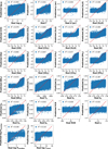 |
Fig. A.1 Real vs. predicted comparison for all included model parameters. The RvP originates from training and testing the random forest on the same grid. No noise is assumed. In each panel, the dashed red line indicates perfect agreement. |
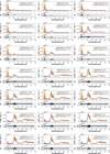 |
Fig. A.2 Posterior retrieval median fits, F (orange line), and residuals, ∆F (black line), associated with the free-chemistry retrieval analyses for the curated brown dwarfs, analogous to Fig. 4, using the preferred cloud model by Bayesian model selection. The retrieved error inflations are represented by a horizontal gray bars. The JWST NIRSpec and MIRI data are shown as blue dots with associated uncertainties. |
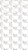 |
Fig. A.3 Retrieved median temperature-pressure profiles and associated 1σ uncertainties for the free-chemistry retrieval analyses of the curated brown dwarfs, analogous to Fig. 3, using the preferred cloud model by Bayesian model selection. Adiabatic profiles (dashed black line) are indicated for comparison. |
Appendix B Posterior tables
For completeness, Tables B.1 to B.4 list the posterior parameters constrained from the BEAR atmospheric retrievals, both using a cloud-free and a gray cloud model. Table B.5 then records all posterior parameters originating from the random forest retrieval study using the HELA framework, which is individually trained on each model grid.
Cloud-free BeAR retrieval outcomes for the curated sample of late-T and Y dwarfs.
gray cloud BeAR retrieval outcomes for the curated sample of late-T and Y dwarfs.
Random forest retrieval outcomes using the HELA framework.
All Tables
Retrieval parameters and prior distributions for the free chemistry approach used in the cloud-free and non-gray cloud models.
Bayesian statistics for the retrieval analysis of the curated set of brown dwarfs.
Cloud-free BeAR retrieval outcomes for the curated sample of late-T and Y dwarfs.
gray cloud BeAR retrieval outcomes for the curated sample of late-T and Y dwarfs.
All Figures
|
Fig. 1 Spectral sample of 22 T and Y dwarfs originally published in Beiler et al. (2024a). All spectra have been normalized at their maximum flux value and offset by a constant. |
| In the text | |
|
Fig. 2 Feature importance across wavelengths for all parameters included in our generated model grid for the case study of the Y1 dwarf WISEPAJ1541-22 as well as their joint retrieval. The significance of a feature is quantified by the normalized decrease in variance it generates throughout the training process. Specifically, it denotes the total reduction in variance achieved whenever that feature is employed for partitioning nodes in a decision tree within the ensemble. For visual guidance, the rescaled spectrum of WISEPAJ1541-22 is overlaid as solid black lines. |
| In the text | |
|
Fig. 3 Joint posterior distributions from the free-chemistry retrieval analyses of the case study Y1 dwarf WISEPAJ1541-22 using a gray cloud model. The vertical dashed lines within the histograms indicate the median parameter values and their 1σ uncertainties. Accompanying the montage of joint posterior distributions is the retrieved median temperature-pressure profile along with its associated 1σ uncertainties. The adiabatic profile (dashed black line) is indicated for comparison. |
| In the text | |
|
Fig. 4 Posterior retrieval median fit, F (orange line), and residuals, ∆F (black line), associated with the free-chemistry retrieval analyses of the case study Y1 dwarf WISEPAJ1541-22 using a gray cloud model. The retrieved error inflation is represented by a horizontal gray bar. The JWST NIRSpec and MIRI data are shown as blue dots with associated uncertainties. |
| In the text | |
|
Fig. 5 Normalized carbon-to-oxygen (C/O) ratio probabilities expressed relative to the solar value of 0.5 5 ± 0.09 (Asplund et al. 2009) for the case study Y1 dwarf WISEPAJ1541-22. Prior (red) and posterior (orange) probability distributions were derived from combinations of molecular gas abundance distributions. The solar value is indicated with a dashed blue line and shaded region. |
| In the text | |
|
Fig. 6 Chemical composition for Y1 dwarf WISEPAJ1541-22 calculated with FastChem. The upper panel shows the volume mixing ratios of major gas-phase species. Retrieved abundances from the BeAR retrieval and their 1σ confidence intervals are depicted by the shaded areas. Stable condensates are shown in the lower panel. Their number densities, nc, refer to the effective molecule number contained in the condensed phase and do not correspond to an actual cloud particle number density. The cloud top position and its 1σ confidence interval constrained by the retrieval calculations ( |
| In the text | |
|
Fig. 7 Comparison of retrieved posterior outcomes for effective temperature (top), surface gravity (middle), and radii (bottom) from our suite of brown dwarf retrievals across the T-Y sequence. The brown dwarfs are ordered with respect to their spectral class, from T6 to Y1 (see Table 1 for details). For each object within the curated sample, all permutations of the theoretical grid models, which were used for training the HELA random forest routine, are shown as well as the posterior parameters retrieved by using the nested sampling BeAR framework. For each posterior, the 1σ uncertainties are shown, but they are too small to be visible for the BeAR posteriors. Gray bars in the top panel indicate the effective temperature values determined by Beiler et al. (2024a) using integrated luminosities and radii from evolutionary models (see their Table 4). |
| In the text | |
|
Fig. 8 Posterior BeAR retrieval values for molecular log-volume mixing ratios (log VMR) of H2O, CH4, NH3, K, CO2, and CO plotted against the retrieved effective temperature (Teff; shown in red). For visual comparison, modeled volume mixing ratios from the Sonora Elf Owl model grid (Mukherjee et al. 2024) are overlaid for a surface gravity of log g = 5.0 (cgs units) and a vertical eddy diffusion coefficient of log κzz = 8.0 with varying metallicities ([M/H]) and carbon-to-oxygen (C/O) ratios relative to solar. |
| In the text | |
|
Fig. A.1 Real vs. predicted comparison for all included model parameters. The RvP originates from training and testing the random forest on the same grid. No noise is assumed. In each panel, the dashed red line indicates perfect agreement. |
| In the text | |
|
Fig. A.2 Posterior retrieval median fits, F (orange line), and residuals, ∆F (black line), associated with the free-chemistry retrieval analyses for the curated brown dwarfs, analogous to Fig. 4, using the preferred cloud model by Bayesian model selection. The retrieved error inflations are represented by a horizontal gray bars. The JWST NIRSpec and MIRI data are shown as blue dots with associated uncertainties. |
| In the text | |
|
Fig. A.3 Retrieved median temperature-pressure profiles and associated 1σ uncertainties for the free-chemistry retrieval analyses of the curated brown dwarfs, analogous to Fig. 3, using the preferred cloud model by Bayesian model selection. Adiabatic profiles (dashed black line) are indicated for comparison. |
| In the text | |
Current usage metrics show cumulative count of Article Views (full-text article views including HTML views, PDF and ePub downloads, according to the available data) and Abstracts Views on Vision4Press platform.
Data correspond to usage on the plateform after 2015. The current usage metrics is available 48-96 hours after online publication and is updated daily on week days.
Initial download of the metrics may take a while.