| Issue |
A&A
Volume 707, March 2026
|
|
|---|---|---|
| Article Number | A238 | |
| Number of page(s) | 16 | |
| Section | Planets, planetary systems, and small bodies | |
| DOI | https://doi.org/10.1051/0004-6361/202556365 | |
| Published online | 17 March 2026 | |
An Earth-sized planet on a 5.4 h orbit around a nearby K dwarf
1
Anton Pannekoek Institute for Astronomy, University of Amsterdam,
Science Park 904,
1098
XH
Amsterdam,
The Netherlands
2
Instituto de Astrofísica, Pontificia Universidad Católica de Chile,
Av. Vicuña Mackenna 4860,
782-0436
Macul, Santiago,
Chile
3
Millennium Institute for Astrophysics,
Santiago,
Chile
4
Jet Propulsion Laboratory, California Institute of Technology,
4800 Oak Grove Drive,
Pasadena,
CA
91109,
USA
5
Department of Astronomy & Astrophysics, 525 Davey Laboratory, The Pennsylvania State University,
University Park,
PA
16802,
USA
6
Center for Exoplanets and Habitable Worlds, 525 Davey Laboratory, The Pennsylvania State University,
University Park,
PA
16802,
USA
7
Institute for Computational and Data Sciences, The Pennsylvania State University,
University Park,
PA
16802,
USA
8
Center for Astrostatistics, 525 Davey Laboratory, The Pennsylvania State University,
University Park,
PA
16802,
USA
9
U.S. National Science Foundation National Optical-Infrared Astronomy Research Laboratory,
950 N. Cherry Avenue,
Tucson,
AZ
85719,
USA
10
NASA Goddard Space Flight Center,
Greenbelt,
MD
20771,
USA
11
Australian Astronomical Optics, Macquarie University,
Balaclava Road,
North Ryde,
NSW
2109,
Australia
12
Astrophysics and Space Technologies Research Centre, Macquarie University,
Balaclava Road,
North Ryde,
NSW
2109,
Australia
13
School of Mathematical and Physical Sciences, Macquarie University,
Balaclava Road,
North Ryde,
NSW
2109,
Australia
14
Department of Physics and Astronomy, University of Pennsylvania,
209 South 33rd Street,
Philadelphia,
PA
19104,
USA
15
Center for Computational Astrophysics, Flatiron Institute,
162 Fifth Avenue,
New York,
NY
10010,
USA
16
Department of Astronomy, University of Illinois at Urbana-Champaign,
Urbana,
IL
61801,
USA
17
Department of Physics and Astronomy, Amherst College,
Amherst,
MA
01002,
USA
18
Earth and Planets Laboratory, Carnegie Institution for Science,
5241 Broad Branch Road, NW,
Washington,
DC
20015,
USA
19
Steward Observatory, University of Arizona,
933 N. Cherry Ave,
Tucson,
AZ
85721,
USA
20
Department of Astronomy and Astrophysics, Tata Institute of Fundamental Research,
Homi Bhabha Road, Colaba,
Mumbai
400005,
India
21
Department of Physics & Astronomy, The University of California, Irvine,
Irvine,
CA
92697,
USA
22
McDonald Observatory and Center for Planetary Systems Habitability, The University of Texas at Austin,
Austin,
TX
78730,
USA
23
Department of Astrophysical Sciences, Princeton University,
4 Ivy Lane,
Princeton,
NJ
08540,
USA
★ Corresponding author: This email address is being protected from spambots. You need JavaScript enabled to view it.
Received:
11
July
2025
Accepted:
15
December
2025
Abstract
We present the discovery and confirmation of the ultrashort period (USP) planet TOI-2431 b orbiting a nearby (d ~ 36 pc) late K star (Teff = 4109 ± 28 K) using observations from the Transiting Exoplanet Survey Satellite (TESS), precise radial velocities (RVs) with NEID and Habitable-zone Planet Finder (HPF) spectrographs, as well as ground-based high-contrast imaging from NESSI. TOI-2431 b has a period of 5 hours and 22 minutes, making it one of the shortest-period exoplanets known to date. TOI-2431 b has a radius of 1.534 ± 0.033 R⊕ and a mass of 6.2 ± 1.6 M⊕, where the exact mass precision shows a slight dependence on the choice of prior. This suggests TOI-2431 b has a density compatible with an Earth-like composition and due to its high irradiation, it is likely to be a “lava-world” with a Teq = 2063 ± 30 K. We estimate that the current orbital period is only 30% larger than the Roche-limit orbital period and that it has an expected orbital decay timescale of only ~31 Myr. Finally, due to the brightness of the host star (V = 10.9, K = 7.6), we find that TOI-2431 b has a high emission spectroscopy metric (ESM) of 27, making it one of the best USP systems for atmospheric phase-curve analyses.
Key words: techniques: photometric / techniques: radial velocities / planets and satellites: detection / planets and satellites: general / planets and satellites: terrestrial planets
President’s Postdoctoral Fellow.
© The Authors 2026
 Open Access article, published by EDP Sciences, under the terms of the Creative Commons Attribution License (https://creativecommons.org/licenses/by/4.0), which permits unrestricted use, distribution, and reproduction in any medium, provided the original work is properly cited.
This article is published in open access under the Subscribe to Open model. This email address is being protected from spambots. You need JavaScript enabled to view it. to support open access publication.
1 Introduction
Ultrashort period (USP) planets have orbital periods of less than one day (Sahu et al. 2006; Adams et al. 2016; Goyal & Wang 2025). Of the ~6000 exoplanets discovered so far, about 150 are confirmed USP planets as per the NASA Exoplanet Archive1 (Akeson et al. 2013; Christiansen et al. 2025). Most USP planets have radii <2 R⊕ (Winn et al. 2018). They tend to have Earth-like compositions (Dai et al. 2019), although some are consistent with compositions enhanced in iron as compared to the Earth (Price & Rogers 2020; Uzsoy et al. 2021). Due to their close-in orbits, USP planets tend to have surface temperatures in excess of 2000 K, suggesting their surfaces are likely molten.
Using data from the Kepler mission, Sanchis-Ojeda et al. (2014) found that the occurrence rate of USP planets is 1.1 ± 0.4% for M dwarfs, 0.51 ± 0.07% for G dwarfs, and only 0.15 ± 0.05% for F dwarfs, suggesting that the presence of a USP planet depends on the spectral type of the star. Furthermore, Winn et al. (2018) noted that USP planets are often found in compact multiplanet systems, with high orbital period ratios, where the orbital period of the innermost USP planet and its closest neighbor typically has a ratio of 4 or more (Steffen & Farr 2013; Winn et al. 2018; Pu & Lai 2019). This ratio is larger than the value generally seen in multiplanet systems discovered by Kepler (Fabrycky et al. 2017). Furthermore, Dai et al. (2018) showed that the dispersion of orbital inclinations among transiting planets tends to be larger when a USP planet is part of the system.
The origin of USP planets is not fully understood and a few different formation scenarios have been proposed. One scenario assumes that rocky USP planets represent the exposed cores of hot Jupiters (Jackson et al. 2013; Valsecchi et al. 2015; Königl et al. 2017). However, Winn et al. (2017) found the metallicity distribution of USP-planet host stars to be different from those of hot Jupiter host stars. In addition, they found that the metallicity distributions of stars hosting rocky USP planets and stars hosting 2–4 R⊕ planets, with orbital periods of a few days are identical. From this perspective, USPs could represent the exposed cores of such smaller (2–4 R⊕) gaseous planets and/or super-Earths (e.g., Lundkvist et al. 2016; Lee & Chiang 2017). Since USP planets are typically found in the star’s dust sublimation region, it is unlikely that they formed at their present location (Murgas et al. 2022) and, therefore, likely migrated to their current orbits. A number of USP migration mechanisms have been proposed, most involving tidal dissipation from different sources and initial conditions (Schlaufman et al. 2010; Lee & Chiang 2017). Petrovich et al. (2019) studied compact multiplanet systems and proposed the possibility of eccentricity excitation from secular dynamical chaos. Pu & Lai (2019) suggested that the outer planets tidally interact with each other and with the innermost planet, damping its eccentricity to close to zero and shrinking its semi-major axis in a quasi-equilibrium state. Millholland & Spalding (2020) proposed that obliquity-driven tidal migration could be a way to obtain USP orbits. Finally, Tu et al. (2025) found that the occurrence of USP planets increases with stellar age, suggesting that different tidal migration pathways may be responsible for younger and older USP planets.
Due to their close-in and short-period orbits, USP planets are some of the most favorable systems for thermal phase-curve and secondary eclipse observations. Owing to their high stellar irradiation, it is likely that any hydrogen-helium (H/He) atmosphere they may have had, has been completely stripped away (Sanchis-Ojeda et al. 2014; Lundkvist et al. 2016; Lopez 2017). Their atmospheric and surface characteristics (e.g., albedo, phase shifts, and temperature differences between the day-and night sides) can shed light on the primary surface mineralogy and/or the presence of a secondary atmosphere (Hu et al. 2012; Demory et al. 2016; Kreidberg et al. 2019; Whittaker et al. 2022; Zhang et al. 2024; Dai et al. 2024).
The Transiting Exoplanet Survey Satellite (TESS; Ricker et al. 2014) has enabled the detection of USP planets around nearby bright stars, facilitating precise mass constraints with ground-based Doppler spectroscopy, as well as phase-curve observations with JWST. LHS 3844 b (Vanderspek et al. 2019), a rocky super-earth orbiting an M dwarf 15 pc away, was the first USP planet found by TESS, and more recent discoveries include GJ 367 b (Lam et al. 2021), TOI-6255 b (Dai et al. 2024), and TOI-6324 b (Lee et al. 2025).
In this paper, we present the discovery of TOI-2431 b, a USP planet with a period of ~0.224 days, making it the sixth shortest period planet known to date. TOI-2431 is a bright (V = 10.9 mag, K = 7.6 mag) K7V star at a distance of 36 pc. TOI-2431 was identified as a TESS objects of interest and statistically validated by Guerrero et al. (2021). Here, we present a detailed characterization of the system, including precise radial velocity (RV) follow-up observations to determine its mass and thereby confirming its planetary nature. Additionally, due to the short period of the planet, we show that TOI-2431 b is very close to its Roche limit, and has one of the highest emission spectroscopy metrics (ESM; Kempton et al. 2018), with JWST enabling high signal-to-noise-ratio (S/N) phase-curve observations.
This paper is structured as follows. In Section 2, we describe the observations and data reduction. In Section 3, we discuss the parameters of the host star. In Section 4, we discuss the Transit and RV joint analysis, and we present our planet parameter constraints in Section 5. In Section 6, we discuss our search for additional planets in the system, as well as the composition, tidal decay, tidal distortion, and potential for future observations of TOI-2431 b. We conclude with a summary of our findings in Section 7.
2 Observations and data reduction
2.1 TESS photometry
TOI-2431 was observed by TESS in Sectors 31, 42, 43, 70, and 71 at a cadence of two minutes between 2020 and 2023. The TESS Science Processing Operations Center (SPOC, Jenkins et al. 2016) pipeline identified a small transit signal with a periodicity of ~5 hours. We downloaded and combined the available light curves using the lightkurve package (Lightkurve Collaboration 2018). We worked with the Presearch Data Conditioning Simple Aperture Photometry (PDC-SAP) SPOC light curves, which are corrected for pointing and focus-related instrumental signatures, discontinuities resulting from radiation events in the CCD detectors, outliers, and flux contamination. Figure 1 shows the TESS pixels used for the PDC light curve generated with the tpfplotter code2. The TESS light curve, along with the best transit model, is shown in Section 4.1.
2.2 Radial velocities with NEID and HPF
To constrain the mass of TOI-2431 b, we obtained high precision RVs using the NEID spectrograph (Schwab et al. 2016) on the WIYN 3.5 m Telescope3 at Kitt Peak National Observatory in Arizona. In total, we obtained 12 NEID exposures between December 17, 2024 and February 19, 2025. The exposure time for all observations was 5 minutes. The S/N varied per observation, with the median S/N of 27 at 860 nm.
The NEID spectra were first extracted using the NEID Data Reduction Pipeline (DRP4; Bender et al. 2022). These spectra were downloaded from the NEID archive5. We then extracted RVs from NEID using the NEID-SERVAL code, a spectral-matching code that builds on the SpEctrum Radial Velocity AnaLyzer (SERVAL; Zechmeister et al. 2018) code and that has been adapted for NEID data (Stefànsson et al. 2022). On this basis, we obtained a median RV precision of 2.9 m s−1.
In addition to the NEID data, to constrain the stellar parameters of the host star, we also obtained spectra of TOI-2431 with the Habitable-zone Planet Finder (HPF) Spectrograph (Mahadevan et al. 2012) on the 10 m Hobby-Eberly Telescope (HET, Ramsey et al. 1988; Hill et al. 2021) at McDonald Observatory in Texas. We obtained three observations between December 29, 2024, and February 9, 2025, using ~15 minute exposures. For these observations, the median S/N is 205 at 1 μm with the median RV precision of 7.3 m s−1.
The HPF 1D spectra were first reduced and extracted using the HPF pipeline, following the procedures outlined in Ninan et al. (2018), Kaplan et al. (2019), and Metcalf et al. (2019). We extracted the RVs using HPF-SERVAL following Stefansson et al. (2020) and Stefánsson et al. (2023). The RVs of TOI-2431 are listed in Table B.1.
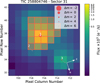 |
Fig. 1 TESS target pixel file image of TOI-2431 in Sector 31. The electron fluxes are shown with the color bar. The red-bordered pixels highlight the pixels used for the PDCSAP light curve. The TESS pixel scale is approximately 21″. The size of the red circles indicates the TESS magnitudes of all nearby stars and TOI-2431 (white cross). Gray arrows show the proper motion directions of the stars in the field. |
2.3 Speckle imaging
To rule out the presence of nearby stars to TOI-2431, we observed TOI-2431 using the NESSI speckle imager (Scott et al. 2018) on the WIYN 3.5 m Telescope at Kitt Peak in Arizona in two bands: the 562 nm band (width of 44 nm), and the 832 nm band (width of 40 nm; Scott et al. 2018) available on NESSI. Figure 2 shows the reconstructed images in both bands along with the corresponding 5σ contrast curve. The figure shows that no secondary sources were detected near (between 0.2″ and 1.2″) the host star.
TOI-2431 is a high proper motion star, with a total proper motion of 384.5 mas yr−1 (μα = 374.9 mas yr−1, μδ = −85.7 mas yr−1; Gaia Collaboration 2023). Thus, to rule out any background star contamination as TOI-2431 moves across the sky, we also inspected the movement of TOI-2431 as a function of time, as seen in Fig. 3. For this, we have used the First Palomar Sky Survey (POSS-I; Deacon et al. 2009) image taken in 1954 and an image taken by the Zwicky Transient Facility (ZTF; Masci et al. 2019) in 2018. To compare the images, we have also highlighted the position of TOI-2431 as measured by Gaia (Gaia Collaboration 2023) at the Gaia J2016 epoch. The comparison showed that TOI-2431 has moved substantially from 1954 to 2018 and there are no background stars around it that could affect our interpretation.
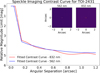 |
Fig. 2 Results from NESSI speckle imaging of TOI-2431. The plot shows the contrast curve as observed in the NESSI 562 nm filter (blue curve), and the 832 nm filter (red). The inset images highlight 256 × 256 insets of the reconstructed images. No secondary companions are seen. Note that in this figure, 1″corresponds to 36 AU at the distance of TOI-2431 b. |
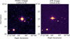 |
Fig. 3 Movement of TOI-2431 as a function of time. Left: POSS-I image of TOI-2431 (middle star) taken in 1954. Right: ZTF image of TOI-2431 taken in 2018. The red circle highlights the position of TOI-2431 as measured by Gaia at the Gaia J2016 epoch. Due to its high proper motion, TOI-2431 has moved substantially between the two images, highlighting that there is no background star seen in the vicinity of TOI-2431 that could confound the planet interpretation of TOI-2431 b. |
3 Stellar parameters
3.1 Spectroscopic and model dependent stellar parameters
We used the HPF-SpecMatch code (Stefansson et al. 2020) to constrain the stellar effective temperature (Teff), surface gravity (log g), and metallicity ([Fe/H]) of TOI-2431. HPF-SpecMatch compares an observed spectrum of a target star with a library of high S/N HPF spectra of well-characterized stars. For the analysis, we followed Stefansson et al. (2020) and used the fifth HPF spectral order, which spans 8534–8645 Å, as this order is the HPF order that is minimally impacted by telluric and sky-emission line contamination. Using HPF-SpecMatch, we obtained Teff = 4080 ± 59 K, log g = 4.68 ± 0.04, and [Fe/H] = −0.02 ± 0.16 dex, where the uncertainties are obtained with the cross-validation approach outlined in Stefansson et al. (2020) and Jones et al. (2024).
To obtain model-dependent estimates of the other stellar parameters of interest, including the mass, radius, and age of the host star, we made use of the ARIADNE code (Vines & Jenkins 2022) to fit the spectral energy distribution (SED) of the host star. To fit the SED, ARIADNE uses the Bayesian model averaging technique on a suite of different possible stellar models. For the fit, we used the Phoenix v2 (Husser et al. 2013), BT-Settl (Allard et al. 2012), Kurucz (1993), and Castelli & Kurucz (2003) stellar atmospheric models. We have also placed informative priors on Teff, [Fe/H], and log g, from the HPF-SpecMatch analysis above. Given the proximity of the star, we assumed that the optical interstellar extinction was negligible and set the corresponding extinction parameter, Av, to zero. Within ARIADNE, we adopted the default ARIADNE priors on the stellar radius (broad uniform prior ranging from 0.05 R⊙ to 100 R⊙) and the distance to the system (informative Gaussian derived by Bailer-Jones et al. 2021). We list the best-fit parameters obtained from the fit in Table 1. The stellar age and isochrone mass are calculated by ARIADNE using the best-fit parameters and the photometric data as input for a MIST isochrone interpolation (Dotter 2016). Lastly, ARIADNE cross-matches the best fit effective temperature to the spectral type table from Pecaut & Mamajek (2013) to determine the spectral type of the star.
3.2 Stellar activity
The S/N of the NEID spectra are not sufficient to recover the Ca II H & K S-value and ![Mathematical equation: $\[\log R_{H K}^{\prime}\]$](/articles/aa/full_html/2026/03/aa56365-25/aa56365-25-eq1.png) activity indicators, so we could not use these to estimate expected RV jitter due to magnetic activity (Wright 2005; Isaacson & Fischer 2010; Luhn et al. 2020). However, we note that none of the Hα or the three Ca II NIR triplet lines were seen to be in emission, indicating that this star is inactive. Further, the TESS photometry does not show evidence of rotational modulation, which is broad agreement with the lack of detection of a clear rotational broadening in the HPF and NEID spectra (v sin i⋆ < 2 km s−1). Together, these facts support the probability that TOI-2431 is a slowly rotating star that is not expected to show any strong rotational modulation in RVs, especially with respect to timescales close to those of the periodicity of the planet (~5 hours).
activity indicators, so we could not use these to estimate expected RV jitter due to magnetic activity (Wright 2005; Isaacson & Fischer 2010; Luhn et al. 2020). However, we note that none of the Hα or the three Ca II NIR triplet lines were seen to be in emission, indicating that this star is inactive. Further, the TESS photometry does not show evidence of rotational modulation, which is broad agreement with the lack of detection of a clear rotational broadening in the HPF and NEID spectra (v sin i⋆ < 2 km s−1). Together, these facts support the probability that TOI-2431 is a slowly rotating star that is not expected to show any strong rotational modulation in RVs, especially with respect to timescales close to those of the periodicity of the planet (~5 hours).
4 Joint transit and RV analysis
To confirm the planetary nature of TOI-2431 b and to better constrain its parameters, we performed joint fits of all of the available transit and RV data using the juliet code (Espinoza et al. 2019). juliet uses the batman code (Kreidberg 2015) for the transit model, radvel (Fulton et al. 2018) for the RV model, celerite (Foreman-Mackey et al. 2017) for the Gaussian process (GP) modeling, and dynesty (Speagle 2020) for the dynamic nested sampling. We assumed that TOI-2431 b has a circular orbit (e = 0), as we expect the orbit to circularize on a short timescale due to tidal interactions with its host star. Additionally, as the TESS contamination ratio is low at 0.0011 (Jenkins et al. 2016), we assumed no additional dilution of the transit due to nearby stars and we fixed the dilution factor for all TESS photometry to unity in all of our fits. We also attempted a TESS-Gaia Light Curve (TGLC; Han & Brandt 2023) fit, which resulted in transit depths that are consistent within 1σ of the TESS light curve fit. To account for correlated noise in the TESS data, in all of the fits, we used a GP model with a Matern-3/2 kernel as implemented in the celerite code (Foreman-Mackey et al. 2017). Additionally, for the joint fits, we placed an informative prior on the stellar density of ρ⋆ = 3.230 ± 0.180 g/cm3 (see Table 1).
As a separate test, we performed similar fits with two additional codes: with the ironman code (Espinoza-Retamal et al. 2023a, 2024) and with the ExoMUSE6 code, a code we developed, which uses radvel and batman, but also uses Markov chain Monte Carlo (MCMC) sampling using the emcee package (Foreman-Mackey et al. 2013) instead of nested sampling. All fits resulted in consistent parameters within ~1σ and we elected to adopt the parameters we obtained using the juliet code.
We tested fitting the available NEID RV data assuming a single Keplerian, using informative priors on the orbital period of the planet and the transit mid-point from the TESS data. However, this resulted in a residual RV RMS scatter of 9.2 m s−1 that is substantially higher than that expected from the median NEID RV uncertainty of 2.9 m s−1. Since the star shows no clear signs of activity and USP planets are often found in multiplanet systems (Winn et al. 2018), this could suggest the presence of additional nontransiting planets in the system.
As highlighted in Section 6.1, we looked for evidence of additional planets in both the TESS data using a box-least squares (BLS) analysis, and in the RVs, using generalized Lomb-Scargle (GLS) periodograms, but we did not find statistically significant periodic signals in the currently available datasets (Section 6.1 for further details). As highlighted in Section 6.1, we attribute the lack of periodic signals detected in the GLS analysis of the RVs due to the low total number of RVs (12 RVs) and urge additional RV observations to characterize any periodicities in the RV data.
To constrain the mass of TOI-2431 b, we used joint transit and RV fits using two different approaches to account for the excess RV scatter: a) a joint transit and RV fit using the floating chunk offset (FCO) method for the RVs and b) a joint transit and RV fit employing both (i) a Keplerian for the innermost planet and (ii) a quasi-periodic GP noise model to account for the excess RV scatter at longer periodicities than the USP. We discuss the results from the two fits below.
4.1 Joint fit employing the FCO method
As USP planets tend to be found in multiplanetary systems, which could cause the RV data to be scattered in excess of the USP RV orbit, an often-used technique to account for the additional RV scatter is the FCO method. The method was originally used by Hatzes et al. (2010) to measure the mass of CoRoT-7b, a USP planet with a 0.85 day period and it has been repeatedly used since then to measure the masses for multiple short-period planets in the presence of other signals (Hatzes 2014; Deeg et al. 2023; Dai et al. 2024).
The FCO method requires multiple observations to be taken over a single night spanning orbital phases that cause measurable velocity differences. It assumes a Keplerian RV orbit for the innermost planet and fits independent RV offsets between successive visits. Therefore, the method assumes that the only RV motion between successive visits (i.e., within a night) is dominated by the Keplerian model and that the RV impact of other planetary signals are effectively removed by fitting the RV offsets. For TOI-2431 b, since the period is only 5.4 hours, we obtained eight RV observations in three different visits, which had typical time-baseline of ~1–2 hours within a visit, with a total time-baseline of ~64 days.
We further note that although we do not expect significant RV variability on the rotational time scale for TOI-2431 given that it is an inactive star (Section 3.2), the FCO method will also remove any activity-driven RV signals at the stellar rotation period. Furthermore, as TOI-2431 is an inactive star, we expect any sources of stellar variability within a night (e.g., oscillations, granulation) that would be retained via the FCO method are also expected to be small and much less than the median RV uncertainty of the NEID data of 2.9 m s−1.
We implemented the FCO method in our joint fits by defining different nights of observations as different “instruments” that had different systematic velocities called NEID1, NEID2, and NEID3. We tried both uniform and log-uniform priors for the jitter terms. For the uniform run, where we adopted a start and stop prior limits of 0.001 and 10 m s−1 (see Table 2), we obtained jitter posteriors of 3.7 m s−1, 4.2 m s−1, 2.9 m s−1 with a semi-amplitude of K = 8.2 ± 2.1 m s−1. For the log-uniform run, where we adopted starting and stop prior limits of 0.001 and 100 m s−1 to allow the samplers to explore even higher jitter values, this resulted in jitter posteriors of 0.13 m s−1, 0.12 m s−1, 0.089 m s−1 with a semi-amplitude of K = 8.2 ± 1.7 m s−1. Both runs resulted in the same parameters, except the uncertainty in the semi-amplitude was larger in the former case. To account for any possibility of additional planets in the system potentially increasing the effective RV jitter, we elected to conservatively adopt the values from the uniform prior given its slightly larger mass error. Those values are shown in Table 2.
As we only had three NEID visits to include for the FCO fit, we performed systematic injection and recovery tests to test the robustness of our FCO implementation, which we highlight in Appendix C. In short, we took our observed NEID times-tamps, and injected 1000 synthetic RV signals of two planets: of a USP planet with the same ephemerides as TOI-2431 b and another longer period planet with a period between 0.44 to 22 days. As highlighted in Appendix C, all injections where the period ratio (Pc/Pb) between TOI-2431 b and the injected planet is higher than 8 are fully recovered. In cases where Pc/Pb > ~8 (corresponding to Pc <~ 1.75 days), only 26 injections out of 390 (or ~ 7%) of the injections were not recovered within 3σ. Therefore, we conclude that if there is another planet in the system with a small period ratio, there is a small chance that it would lead to a biased estimate of the mass constraint of TOI-2431 b. For this reason, we urge the community to obtain additional RV followup observations to further assess and constrain the possibility of another planet in the system. The final joint fit is shown in Figure 4. The resulting best-fit parameters and associated priors are shown in Table 2.
Parameters of TOI-2431.
Derived parameters of TOI-2431 b from a joint analysis of available transit and RV data.
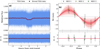 |
Fig. 4 Best-fit results from a joint transit and RV fit using the FCO method for the RV data. a) Detrended TESS photometric observations (2 min exposures) are shown in blue at the top, folded on the time of transit. Best-fit transit model is shown in red. The black points show the TESS data binned to a cadence of 2 min. Residuals from the best-fit model are shown at the bottom. b) Phase-folded RV data and best-fit model (red) of TOI-2431 as observed with NEID in three separate visits listed as NEID1 (blue), NEID2 (yellow), and NEID3 (green), shown at the top. The red-shaded regions show the 1, 2, and 3σ credible intervals of the best-fitting model. Residuals from the best-fit model on the bottom. We adopted the values from this fit as the values for TOI-2431 b. |
4.2 Joint fit employing a quasi-periodic GP
In addition to the FCO fit discussed above, we performed a joint transit and RV fit where we used a GP noise model with a quasi-periodic kernel to account for the excess RV scatter and the possible longer-term RV signals. The kernel function takes the form
![Mathematical equation: $\[k\left(x_l, x_m\right)=\frac{B}{2+C} e^{-\tau / L}\left[\cos \left(\frac{2 \pi \tau}{P_{\mathrm{GP}}}\right)+(1+C)\right],\]$](/articles/aa/full_html/2026/03/aa56365-25/aa56365-25-eq60.png) (1)
(1)
where τ = |xl − xm|, and B, C, L, and PGP are the hyperparameters of the kernel, while B and C are hyperparameters that tune the weight of the exponential decay component of the kernel with a constant of L (in days), and PGP corresponds to the periodicity of the quasiperiodic oscillations (Foreman-Mackey et al. 2017).
To perform the fit, we placed a uniform prior on the periodicity of the quasi-periodic GP from 1 to 100 days, to ensure it was substantially longer than the ~5h period of the Keplerian USP component of the model. To provide the best constraint on the mass, for this fit, we used all of the available NEID RVs, along with the HPF RVs. We note that NEID RVs are more precise than HPF since NEID has higher RV information content on bright K dwarfs than HPF. We let the instrument RV jitters for both instruments float. For consistency, the rest of the priors were kept the same as for the FCO joint fit priors. Table 2 lists the priors and the resulting posterior parameters from the fit, and the resulting GP fit is shown in Figure 5.
5 Results
The results from the FCO joint fit, and the GP joint fits are shown in Figures 4, and 5, respectively. Table 2 lists the resulting posteriors from both fits. The FCO joint fit yields an RV semi-amplitude of ![Mathematical equation: $\[8.2_{-2.1}^{+2.1}\]$](/articles/aa/full_html/2026/03/aa56365-25/aa56365-25-eq61.png) m s−1 and a mass of
m s−1 and a mass of ![Mathematical equation: $\[6.2_{-1.6}^{+1.6}\]$](/articles/aa/full_html/2026/03/aa56365-25/aa56365-25-eq62.png) M⊕. In comparison, the GP joint fit yields an RV semi-amplitude of
M⊕. In comparison, the GP joint fit yields an RV semi-amplitude of ![Mathematical equation: $\[6.8_{-2.0}^{+2.1}\]$](/articles/aa/full_html/2026/03/aa56365-25/aa56365-25-eq63.png) m s−1 and a mass of
m s−1 and a mass of ![Mathematical equation: $\[5.1_{-1.5}^{+1.6}\]$](/articles/aa/full_html/2026/03/aa56365-25/aa56365-25-eq64.png) M⊕.
M⊕.
Both the RV semi-amplitude and mass values are consistent within their 1σ uncertainties, as are the other posterior values (shown in Table 2). As the FCO fit is a simpler fit, with fewer free parameters (one parameter for the Keplerian, three RV offsets, and three RV jitter terms, compared to one Keplerian parameter, two RV offsets, two RV jitter terms, and four parameters for the GP), we elected to adopt the values for the FCO fit. This constrains the mass of the planet at ~3.9σ confirming TOI-2431 b as a USP planet. From Table 2, we see that the FCO joint fit results in a planet radius of ![Mathematical equation: $\[1.534_{-0.033}^{+0.034}\]$](/articles/aa/full_html/2026/03/aa56365-25/aa56365-25-eq65.png) R⊕. This suggests a density of
R⊕. This suggests a density of ![Mathematical equation: $\[9.4_{-2.5}^{+2.5}\]$](/articles/aa/full_html/2026/03/aa56365-25/aa56365-25-eq66.png) g cm−3, which is slightly denser, but consistent with an Earth-like composition.
g cm−3, which is slightly denser, but consistent with an Earth-like composition.
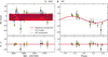 |
Fig. 5 Best fit results from a joint transit and RV fit using a quasi-periodic GP model to account for the excess RV scatter in the RVs. a) NEID (yellow) and HPF (green) RVs as a function of time at the top. The best-fit Keplerian model is shown in red (appears as a solid band due to the short period orbit). The median of the GP component is shown in blue. The joint best-fit model is shown in grey. Residuals from the best fit model, shown at the bottom. b) Phase-folded RVs on the period of TOI-2431 b, shown at the top. Best-fit Keplerian model after subtracting the GP model is in red. RV residuals as a function of phase are shown at the bottom. |
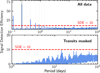 |
Fig. 6 BLS periodogram of the TESS data. Top: BLS periodogram of all of the TESS sectors. The highest peak reveals the period of TOI-2431 b of 0.22 days, which is highlighted with the black dashed vertical line. Aliases of this period are also shown as faint dashed lines. The horizontal red dashed line shows a SDE of 10, the threshold we adopt for a significant signal. Bottom: BLS periodogram of the TESS data after masking out the transits of TOI-2431 b. No significant peaks are detected. |
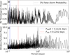 |
Fig. 7 GLS periodogram and window function of the NEID RVs of TOI-2431. a) GLS periodogram. The grey dotted line represents the FAP of 1%. The period of TOI-2431 b is highlighted with red vertical dashed line and the half-period is highlighted with blue vertical dashed line. Beyond the peak seen at Porb/2, we see no additional signals with a FAP< 1%. b) Window function of the RVs shown in panel a. |
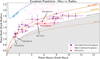 |
Fig. 8 Planet radius as a function of planet mass along with lines of constant density from (Zeng et al. 2019). The gray-shaded region indicates planets with iron content exceeding the maximum value predicted from models of collisional stripping (Marcus et al. 2010). Confirmed USP planets are shown with bold foreground points, and other confirmed exoplanets from the NASA Exoplanet Archive are shown with the faint purple points. TOI-2431 b is shown in red. We only show systems with better than 3σ mass and radius constraints. |
6 Discussion
6.1 Search for additional planets
To search for evidence of additional transiting planets in the TOI-2431 system, we used the BLS algorithm, implemented in the lightkurve package (Lightkurve Collaboration 2018). The resulting BLS periodogram is shown in Figure 6. We did not observe any clear signal in the BLS other than the signals corresponding to TOI-2431 b and its aliases. Furthermore, when removing that signal, no additional signals with a signal detection efficiency (SDE) larger than 10 are detected. We see a potential signal with a period of ~14 days and an SDE of ~9, but we attribute this to the combined effect of the gaps in the TESS data (the signal is close to half of the TESS baseline per sector) and masking of TOI-2431 b transits, which removed a significant number of data points. Therefore, we conclude there are no clear signs of additional transiting planets in the system. The lack of detection of other transiting planets is not unexpected, as the planets in USP systems tend to have a high mutual inclinations (Dai et al. 2018). Together with the high period ratios between neighboring planets (Dai et al. 2015), this can easily explain the nondetection of additional transiting planets in the system.
To look for evidence of nontransiting planets in the RVs, we examined the GLS periodogram of the NEID RVs, along with the accompanying window function in Figure 7. We highlight the orbital period of TOI-2431 b’s with the red vertical dashed line and we highlight half of the orbital period with the blue vertical dashed line. The latter has a false alarm probability (FAP) <1% (grey horizontal line), which we attribute as likely being due to TOI-2431 b. The window function shows that these peaks do not originate from an artifact due to sampling. The grey dotted line shows that we do not detect any additional significant periodicities with FAP <1%. We attribute this being due to the low number of RVs, as periodogram analyses such as these benefit from higher number of datapoints, especially in the absence of extremely clear sinusoidal signals. Given the high RV scatter compared to expectations from a single Keplerian, we urge additional RV observations of the system to look for evidence of significant additional periodicities to reveal additional planets in the TOI-2431 system.
In addition to RVs, massive longer period exoplanets could also be detected using astrometry. The star is included in the HIPPARCOS-Gaia Catalog of Accelerations (Brandt 2021). However, we do not see any significant proper motion differences, ruling out massive companions at large orbital distances. Nonetheless, future Gaia DR4 astrometry can put more constraints on possible outer companions at intermediate orbital distances of ~3–5 AU (Perryman et al. 2014). The star is relatively nearby (d ~ 36 pc) and bright (G ~ 10.3), which increases the likelihood of detecting massive outer companions to TOI-2431 b with Gaia (and possibly measuring the mutual inclination between the planetary orbits; Espinoza-Retamal et al. 2023b).
6.2 Planet composition
Figure 8 compares the mass and radius of TOI-2431 b compared to other USP planets (bold points) and other exoplanets (faint points) with well-characterized masses and radii. To examine possible compositions compatible with TOI-2431 b, we additionally plot planet composition models from Zeng et al. (2019) as lines of constant density. We see that TOI-2431 b is slightly denser, but compatible with an Earth-like planet composition, similar to other well-characterized USP planets. Due to its close distance to the host star and the high incident irradiation, this results in an equilibrium temperature of 2063 ± 30 K (assuming Bond albedo as AB = 0). This temperature exceeds the melting points of many common silicate minerals found in planets, suggesting that the planet’s surface is likely to be partially or fully molten.
6.3 Star-planet tidal interactions
The short orbital period of TOI-2431 b suggests that it is subject to strong tidal interactions with its host star, potentially leading to tidal deformation and orbital decay. We discuss these tidal effects further below, broadly following similar discussions of the USP planets TOI-6255 b (Dai et al. 2024), and TOI-6324 b (Lee et al. 2025).
6.3.1 Proximity to the Roche limit and tidal deformation
The minimum period at which a planet of mean density, ρp, can orbit before being disintegrated by tidal forces is set by the Roche limit. Approximating a planet as an incompressible fluid, this Roche period is given by (Rappaport et al. 2013):
![Mathematical equation: $\[P_{\text {Roche }} \approx 12.6 \mathrm{~h}\left(\frac{\rho_{\mathrm{p}}}{1 \mathrm{~g} \mathrm{~cm}^{-3}}\right)^{-1 / 2} \text {. }\]$](/articles/aa/full_html/2026/03/aa56365-25/aa56365-25-eq67.png) (2)
(2)
Using TOI-2431 b’s bulk density of ρp = ![Mathematical equation: $\[9.4_{-2.5}^{+2.5}\]$](/articles/aa/full_html/2026/03/aa56365-25/aa56365-25-eq68.png) g cm−3, we estimate PRoche =
g cm−3, we estimate PRoche = ![Mathematical equation: $\[4.11_{-0.36}^{+0.48}\]$](/articles/aa/full_html/2026/03/aa56365-25/aa56365-25-eq69.png) h. Therefore, Porb/PRoche =
h. Therefore, Porb/PRoche = ![Mathematical equation: $\[1.31_{-0.14}^{+0.12}\]$](/articles/aa/full_html/2026/03/aa56365-25/aa56365-25-eq70.png) , suggesting that TOI-2431 b has an orbital period only ~30% larger than the Roche limit and that tidal forces are likely to produce measurable effects on the planet.
, suggesting that TOI-2431 b has an orbital period only ~30% larger than the Roche limit and that tidal forces are likely to produce measurable effects on the planet.
One possible effect of the proximity of TOI-2431 b to its host star is to tidal deformation, where the shape of the planet is elongated toward the host star. To quantify this effect, we can describe the planet as an elongated ellipsoid parametrized as having three different radii, R1, R2, and R3, where R1 is the radius of the planet along the axis that points toward the host star, R2 is located along the direction of orbit, and R3 is along the orbit normal. Following Dai et al. (2024), the radii are given by
![Mathematical equation: $\[R_1=R_{\mathrm{vol}}\left(1+\frac{7}{6} \delta R_p\right),\]$](/articles/aa/full_html/2026/03/aa56365-25/aa56365-25-eq71.png) (3)
(3)
![Mathematical equation: $\[R_2=R_{\mathrm{vol}}\left(1-\frac{1}{3} \delta R_p\right),\]$](/articles/aa/full_html/2026/03/aa56365-25/aa56365-25-eq72.png) (4)
(4)
![Mathematical equation: $\[R_3=R_{\mathrm{vol}}\left(1-\frac{5}{6} \delta R_p\right),\]$](/articles/aa/full_html/2026/03/aa56365-25/aa56365-25-eq73.png) (5)
(5)
where δRp is the tidal distortion of the planet and Rvol is the volumetric radius of the planet defined as Rvol ≡ (R1R2R3)1/3. Given its short-period orbit, TOI-2431 b is expected to be tidally locked (Winn et al. 2018), with a rotational period equal to its orbital period, resulting in R1 being hidden from the observer during transit. The radius that is observed during transit therefore is Rtran ≡ (R2R3)1/2, giving rise to the relation
![Mathematical equation: $\[R_{\mathrm{vol}}=R_{\mathrm{tran}}\left(1+\frac{7}{12} \delta R_p\right).\]$](/articles/aa/full_html/2026/03/aa56365-25/aa56365-25-eq74.png) (6)
(6)
Following Dai et al. (2024), the tidal distortion δRp can be calculated using
![Mathematical equation: $\[\delta R_p=h_2 \zeta,\]$](/articles/aa/full_html/2026/03/aa56365-25/aa56365-25-eq75.png) (7)
(7)
![Mathematical equation: $\[\zeta=\frac{M_{\star}}{M_p}\left(\frac{R_p}{a}\right)^3,\]$](/articles/aa/full_html/2026/03/aa56365-25/aa56365-25-eq76.png) (8)
(8)
where Rp is the planetary radius, h2 is the Love number, a is the semi-major axis, and Mp and M⋆ are the masses of the planet and host star, respectively. Following Dai et al. (2024), we adopted a fiducial h2 = 1, from which we find that TOI-2431 b’s volumetric radius is 2.4% larger than the observed transit radius. Further, we find that the difference between the longest axis, R1, and the shortest axis R3 to be (R1 − R3)/R1 = 0.087 ± 0.017. Putting this value into context with other USPs, Figure 9a shows that, under these assumptions, TOI-2431 b is among the most tidally deformed USP planets, along with TOI-6324 b (Lee et al. 2025), KOI-55 b (Charpinet et al. 2011), and TOI-6255 b (Dai et al. 2024).
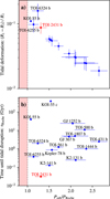 |
Fig. 9 a) Expected tidal deformation of USPs parametrized as a (R1 − R3)/R1 as a function of Porb/PRoche. Here the planets are approximated as compressed ellipsoids with primary axes radii of R1, R2, and R3, where R1 is the radius of the planet pointing toward the star, and R3 is the radius along the orbit normal. We see that TOI-2431 b is among some of the most tidally distorted USP planets. b) Roche limit timescales of USPs as a function of Porb/PRoche. The latter indicates the proximity to the Roche limit, and the former indicates the timescale to reaching the Roche limit. We see that TOI-2431 b has the shortest timescale until tidal disruption of ~31 Myr. |
6.3.2 Orbital decay
Tidal interactions also result in energy dissipation, leading to a gradual inward spiral of a planet toward its host star. The tidal decay timescale, τP, assuming a constant-lag-angle model (Goldreich & Soter 1966; Dai et al. 2024), is given by
![Mathematical equation: $\[\tau_P \equiv \frac{P}{\dot{P}} \approx 30 \operatorname{Gyr}\left(\frac{Q_{\star}^{\prime}}{10^6}\right)\left(\frac{M_{\star} / M_p}{M_{\odot} / M_{\oplus}}\right)\left(\frac{\rho_{\star}}{\rho_{\odot}}\right)^{5 / 3}\left(\frac{P}{1 \text { day }}\right)^{13 / 3},\]$](/articles/aa/full_html/2026/03/aa56365-25/aa56365-25-eq77.png) (9)
(9)
where ![Mathematical equation: $\[Q_{*}^{\prime}\]$](/articles/aa/full_html/2026/03/aa56365-25/aa56365-25-eq78.png) is the reduced stellar tidal quality factor and is the main source of uncertainty for this calculation. Following Dai et al. (2024) and Lee et al. (2025), we adopted
is the reduced stellar tidal quality factor and is the main source of uncertainty for this calculation. Following Dai et al. (2024) and Lee et al. (2025), we adopted ![Mathematical equation: $\[Q_{\star}^{\prime}=10^{7}\]$](/articles/aa/full_html/2026/03/aa56365-25/aa56365-25-eq79.png) , representing a relatively slow stellar dissipation rate as empirically found by Penev et al. (2018). From this, we find τP ≈ 200 Myr for TOI-2431 b, while stressing the underlying uncertainty in the
, representing a relatively slow stellar dissipation rate as empirically found by Penev et al. (2018). From this, we find τP ≈ 200 Myr for TOI-2431 b, while stressing the underlying uncertainty in the ![Mathematical equation: $\[Q_{\star}^{\prime}\]$](/articles/aa/full_html/2026/03/aa56365-25/aa56365-25-eq80.png) value of the star that may differ from the assumed value by more than an order of magnitude and would change the timescale accordingly.
value of the star that may differ from the assumed value by more than an order of magnitude and would change the timescale accordingly.
The time it takes to reach the Roche limit can be found by integrating Equation (9), yielding
![Mathematical equation: $\[\tau_{Roche}=k\left(\left(\frac{P}{1 \text { day }}\right)^{13 / 3}-\left(\frac{P_{Roche}}{1 \text { day }}\right)^{13 / 3}\right),\]$](/articles/aa/full_html/2026/03/aa56365-25/aa56365-25-eq81.png) (10)
(10)
where
![Mathematical equation: $\[k \approx 7 ~\operatorname{Gyr}~\left(\frac{Q_{\star}^{\prime}}{10^6}\right)\left(\frac{M_{\star} / M_p}{M_{\odot} / M_{\oplus}}\right)\left(\frac{\rho_{\star}}{\rho_{\odot}}\right)^{5 / 3},\]$](/articles/aa/full_html/2026/03/aa56365-25/aa56365-25-eq82.png) (11)
resulting in τRoche ≈ 31 Myr. We compare τRoche of TOI-2431 b to other well-characterized USPs in Figure 9b, where we assumed a fixed
(11)
resulting in τRoche ≈ 31 Myr. We compare τRoche of TOI-2431 b to other well-characterized USPs in Figure 9b, where we assumed a fixed ![Mathematical equation: $\[Q_{\star}^{\prime}=10^{7}\]$](/articles/aa/full_html/2026/03/aa56365-25/aa56365-25-eq83.png) for all of the systems, from which we see that TOI-2431 b has the shortest τRoche timescale. This puts TOI-2431 b in a regime where orbital decay could potentially be detectable with long-term observations (see e.g., Wilkins et al. 2017). Such observations will constrain
for all of the systems, from which we see that TOI-2431 b has the shortest τRoche timescale. This puts TOI-2431 b in a regime where orbital decay could potentially be detectable with long-term observations (see e.g., Wilkins et al. 2017). Such observations will constrain ![Mathematical equation: $\[Q_{*}^{\prime}\]$](/articles/aa/full_html/2026/03/aa56365-25/aa56365-25-eq84.png) and could lead to further insights into the tidal interactions and future evolution of the system.
and could lead to further insights into the tidal interactions and future evolution of the system.
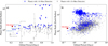 |
Fig. 10 Planet radius as a function of orbital period for known exoplanets. Confirmed planets with a 3σ or higher precision mass detection are highlighted in blue. The planets that have a mass detection smaller than 3σ precision are shown in gray. TOI-2431 b is shown in red. TOI-2431 b is the shortest period planet with both a characterized mass and radius (better than 3σ). a) TOI-2431 b compared to other USPs. b) Same as panel a, but comparing TOI-2431 b to the broader exoplanet population showing that TOI-2431 b is at the lower edge of the hot Neptune desert. |
6.4 Comparison with other USPs and future observations
With a period of only 5.4 hours, TOI-2431 b is among the shortest-period exoplanets discovered to date, but it is the shortest period planet with both a well-characterized mass and radius. The first and second shortest period planets, PSR J1719-1438 b (P= 2.2 h; Bailes et al. 2011) and M62H b (P = 3.2 h; Vleeschower et al. 2024), were discovered with the pulsar timing method, which lacks planetary radius measurements. As for the third and fourth shortest-period planets, KOI-1843.03 (P = 4.2 h; Rappaport et al. 2013) and K2-137 b (P = 4.3 h; Smith et al. 2018), both were discovered by the transit technique, but currently lack robust planet mass measurements. The fifth shortest period planet, KIC 10001893 b (P = 5.3 h; Silvotti et al. 2014), has been discovered with the orbital brightness modulation technique and lacks planetary mass and radius measurements.
The closest exoplanets to TOI-2431 b in terms of period and orbital parameters are TOI-6255 b (P = 5.7 h; Dai et al. 2024), TOI-6324 b (P = 6.7 h; Lee et al. 2025), K2-137 b (P = 4.3 h; Smith et al. 2018), HD 80653 b (P = 17.3 h; Frustagli, G. et al. 2020), and K2-141 b (P = 6.7 h; Malavolta et al. 2018) which were all first detected using the transit technique. As seen in Figure 10, TOI-2431 b is one of the USP planets that form the lower boundary of the hot Neptune desert, which is a sparsely populated region in the exoplanet population (Mazeh et al. 2016).
With its ultrashort period and the brightness of its host star, TOI-2431 b is a promising candidate for phase-curve observations with JWST. Figure 11 shows the ESM (Kempton et al. 2018), which quantifies the feasibility of phase-curve and emission spectroscopic observations with JWST, as a function of orbital period for TOI-2431 b compared to other well-characterized USP planets. TOI-2431 b has an ESM ~ 27 (Table 2), which makes it one of the best rocky planets for phase-curve observations. Such JWST phase-curve observations could shed light onto the presence or absence of a heavy-mean-molecular-weight atmosphere on TOI-2431 b (Dai et al. 2024). In the presence of an atmosphere, JWST’s ability to detect thermal emission across a broad wavelength range would allow a probe of the temperature distribution difference between the dayside and nightside of the planet, yielding insight into the atmospheric circulation of the planet. In the case of no atmosphere, phase-curve observations could inform about the planet’s surface mineralogy, yielding valuable insights into its composition and evolutionary history (Zilinskas, M. et al. 2022; Zhang et al. 2024; Whittaker et al. 2022).
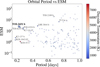 |
Fig. 11 JWST Emission Spectroscopy Metric (ESM) (Kempton et al. 2018) as a function of planet orbital period for TOI-2431 b and other confirmed USP planets. TOI-2431 b is highlighted with the star, and other well-characterized USPs are shown with the thicker labels. The color bar shows the dayside equilibrium temperature assuming an albedo of AB = 0. |
7 Conclusions
We have confirmed the USP planet TOI-2431 b using a combination of photometric transit data from TESS, precise RV observations with the NEID and HPF spectrographs, and ground-based speckle imaging with the NESSI instrument. With a period of P = 0.224 days, TOI-2431 b is among the shortest period exoplanets detected to date. From a joint analysis the available transit data and RVs, we measured a radius of Rp = 1.534 ± 0.033 R⊕ and a mass of Mp = 6.2 ± 1.6 M⊕, suggesting a bulk density of ![Mathematical equation: $\[9.4_{-2.5}^{+2.5}\]$](/articles/aa/full_html/2026/03/aa56365-25/aa56365-25-eq85.png) g/cm3, which is slightly denser, but consistent with an Earth-like composition. The planet has an equilibrium temperature of 2063 ± 30 K (assuming a Bond albedo as AB = 0), suggesting the surface is likely molten. We note that we see evidence of excess scatter in our RV data, compared to a single Keplerian planet model, which we interpret as compelling evidence that there are likely to be other nontransiting planets in the system. We urge additional RV follow-up observations to gain further insights into other planets in the system.
g/cm3, which is slightly denser, but consistent with an Earth-like composition. The planet has an equilibrium temperature of 2063 ± 30 K (assuming a Bond albedo as AB = 0), suggesting the surface is likely molten. We note that we see evidence of excess scatter in our RV data, compared to a single Keplerian planet model, which we interpret as compelling evidence that there are likely to be other nontransiting planets in the system. We urge additional RV follow-up observations to gain further insights into other planets in the system.
Additionally, we show that TOI-2431 b is close to its Roche limit with Porb ≈ 1.31 PRoche. Due to its close-in orbit, we show that TOI-2431 b is likely tidally deformed, with its shortest axis being ~9% shorter than its longest axis. Furthermore, assuming a nominal tidal quality factor of ![Mathematical equation: $\[Q_{\star}^{\prime}=10^{7}\]$](/articles/aa/full_html/2026/03/aa56365-25/aa56365-25-eq86.png) , we estimate a tidal decay timescale of only τRoche ≈ 31 Myr, which is the shortest tidal decay timescale compared to other known USPs.
, we estimate a tidal decay timescale of only τRoche ≈ 31 Myr, which is the shortest tidal decay timescale compared to other known USPs.
Finally, we show that TOI-2431 b has an ESM of 27, making it one of the best USP planets for phase-curve observations with JWST. It could help shed light onto the surface composition and explore whether the planet has an atmosphere.
Data availability
A reproduction package can be found on Zenodo under DOI 10.5281/zenodo.16984082. The package includes the RV and transit data alongside the scripts we have used to do FCO and GP fits as well as planet injection and recovery tests. The package also includes Jupyter notebooks that reproduce all the figures given in this paper. Table B.1 and the light curve data are available at the CDS via https://cdsarc.cds.unistra.fr/viz-bin/cat/J/A+A/707/A238.
References
- Adams, E. R., Jackson, B., & Endl, M. 2016, AJ, 152, 47 [Google Scholar]
- Akeson, R. L., Chen, X., Ciardi, D., et al. 2013, PASP, 125, 989 [Google Scholar]
- Allard, F., Homeier, D., & Freytag, B. 2012, Philos. Trans. R. Soc. A Math. Phys. Eng. Sci., 370, 2765 [Google Scholar]
- Bailer-Jones, C. A. L., Rybizki, J., Fouesneau, M., Demleitner, M., & Andrae, R. 2021, AJ, 161, 147 [Google Scholar]
- Bailes, M., Bates, S. D., Bhalerao, V., et al. 2011, Science, 333, 1717 [NASA ADS] [CrossRef] [Google Scholar]
- Bender, C., Ninan, J., Terrien, R., et al. 2022, Bulletin of the AAS, 54, 6 [Google Scholar]
- Brandt, T. D. 2021, ApJS, 254, 42 [NASA ADS] [CrossRef] [Google Scholar]
- Castelli, F., & Kurucz, R. L. 2003, IAU Symp., 210, A20 [Google Scholar]
- Charpinet, S., Fontaine, G., Brassard, P., et al. 2011, Nature, 480, 496 [NASA ADS] [CrossRef] [Google Scholar]
- Christiansen, J. L., McElroy, D. L., Harbut, M., et al. 2025, arXiv e-prints [arXiv:2506.03299] [Google Scholar]
- Dai, F., Winn, J. N., Arriagada, P., et al. 2015, ApJ, 813, L9 [NASA ADS] [CrossRef] [Google Scholar]
- Dai, F., Masuda, K., & Winn, J. N. 2018, ApJ, 864, L38 [NASA ADS] [CrossRef] [Google Scholar]
- Dai, F., Masuda, K., Winn, J. N., & Zeng, L. 2019, ApJ, 883, 79 [NASA ADS] [CrossRef] [Google Scholar]
- Dai, F., Howard, A. W., Halverson, S., et al. 2024, AJ, 168, 101 [NASA ADS] [CrossRef] [Google Scholar]
- Deacon, N. R., Groot, P. J., Drew, J. E., et al. 2009, MNRAS, 397, 1685 [Google Scholar]
- Deeg, H. J., Georgieva, I. Y., Nowak, G., et al. 2023, A&A, 677, A12 [NASA ADS] [CrossRef] [EDP Sciences] [Google Scholar]
- Demory, B.-O., Gillon, M., de Wit, J., et al. 2016, Nature, 532, 207 [NASA ADS] [CrossRef] [Google Scholar]
- Dotter, A. 2016, ApJS, 222, 8 [Google Scholar]
- Espinoza, N., Kossakowski, D., & Brahm, R. 2019, MNRAS, 490, 2262 [Google Scholar]
- Espinoza-Retamal, J. I., Brahm, R., Petrovich, C., et al. 2023a, ApJ, 958, L20 [NASA ADS] [CrossRef] [Google Scholar]
- Espinoza-Retamal, J. I., Zhu, W., & Petrovich, C. 2023b, AJ, 166, 231 [Google Scholar]
- Espinoza-Retamal, J. I., Stefánsson, G., Petrovich, C., et al. 2024, AJ, 168, 185 [Google Scholar]
- Fabrycky, D. C., Lissauer, J. J., Ragozzine, D., et al. 2017, Architecture of Kepler’s multi-transiting systems. II. New investigations with twice as many candidates., VizieR On-line Data Catalog: J/ApJ/790/146 [Google Scholar]
- Foreman-Mackey, D., Hogg, D. W., Lang, D., & Goodman, J. 2013, PASP, 125, 306 [Google Scholar]
- Foreman-Mackey, D., Agol, E., Ambikasaran, S., Angus, R. 2017, arXiv e-prints [arXiv:1703.09710v2] [Google Scholar]
- Frustagli, G., Poretti, E., Milbourne, T., et al. 2020, A&A, 633, A133 [NASA ADS] [CrossRef] [EDP Sciences] [Google Scholar]
- Fulton, B. J., Petigura, E. A., Blunt, S., & Sinukoff, E. 2018, PASP, 130, 044504 [Google Scholar]
- Gaia Collaboration (Brown, A. G. A., et al.) 2016, A&A, 595, A2 [NASA ADS] [CrossRef] [EDP Sciences] [Google Scholar]
- Gaia Collaboration (Brown, A. G. A., et al.) 2018, A&A, 616, A1 [NASA ADS] [CrossRef] [EDP Sciences] [Google Scholar]
- Gaia Collaboration (Vallenari, A., et al.) 2023, A&A, 674, A1 [NASA ADS] [CrossRef] [EDP Sciences] [Google Scholar]
- Goldreich, P., & Soter, S. 1966, Icarus, 5, 375 [Google Scholar]
- Goyal, A. V., & Wang, S. 2025, AJ, 169, 191 [Google Scholar]
- Guerrero, N. M., Seager, S., Huang, C. X., et al. 2021, ApJS, 254, 39 [NASA ADS] [CrossRef] [Google Scholar]
- Han, T., & Brandt, T. D. 2023, AJ, 165, 71 [NASA ADS] [CrossRef] [Google Scholar]
- Hatzes, A. P. 2014, A&A, 568, A84 [NASA ADS] [CrossRef] [EDP Sciences] [Google Scholar]
- Hatzes, A. P., Dvorak, R., Wuchterl, G., et al. 2010, A&A, 520, A93 [NASA ADS] [CrossRef] [EDP Sciences] [Google Scholar]
- Hill, G. J., Lee, H., MacQueen, P. J., et al. 2021, AJ, 162, 298 [NASA ADS] [CrossRef] [Google Scholar]
- Høg, E., Fabricius, C., Makarov, V. V., et al. 2000, A&A, 355, L27 [Google Scholar]
- Hu, R., Ehlmann, B. L., & Seager, S. 2012, ApJ, 752, 7 [NASA ADS] [CrossRef] [Google Scholar]
- Husser, T.-O., von Berg, S. W., Dreizler, S., et al. 2013, A&A, 553, A6 [NASA ADS] [CrossRef] [EDP Sciences] [Google Scholar]
- Isaacson, H., & Fischer, D. 2010, ApJ, 725, 875 [Google Scholar]
- Jackson, B., Stark, C. C., Adams, E. R., Chambers, J., & Deming, D. 2013, ApJ, 779, 165 [NASA ADS] [CrossRef] [Google Scholar]
- Jenkins, J. M., Twicken, J. D., McCauliff, S., et al. 2016, SPIE Conf. Ser., 9913, 99133E [Google Scholar]
- Jones, S. E., Stefánsson, G., Masuda, K., et al. 2024, AJ, 168, 93 [NASA ADS] [Google Scholar]
- Kaplan, K. F., Bender, C. F., Terrien, R. C., et al. 2019, ASP Conf. Ser., 523, 567 [NASA ADS] [Google Scholar]
- Kempton, E. M.-R., Bean, J. L., Louie, D. R., et al. 2018, PASP, 130, 114401 [CrossRef] [Google Scholar]
- Königl, A., Giacalone, S., & Matsakos, T. 2017, ApJ, 846, L13 [CrossRef] [Google Scholar]
- Kreidberg, L. 2015, PASP, 127, 1161 [Google Scholar]
- Kreidberg, L., Koll, D. D. B., Morley, C., et al. 2019, Nature, 573, 87 [NASA ADS] [CrossRef] [Google Scholar]
- Kurucz, R. 1993, ATLAS9 Stellar Atmosphere Programs and 2 km/s grid. Kurucz CD-ROM No. 13. Cambridge, 13 [Google Scholar]
- Lam, K. W. F., Csizmadia, S., Astudillo-Defru, N., et al. 2021, Science, 374, 1271 [NASA ADS] [CrossRef] [Google Scholar]
- Lee, E. J., & Chiang, E. 2017, ApJ, 842, 40 [Google Scholar]
- Lee, R. A., Dai, F., Howard, A. W., et al. 2025, ApJ, 983, L36 [Google Scholar]
- Lightkurve Collaboration (Cardoso, J. V. d. M., et al.) 2018, Astrophysics Source Code Library [record ascl:1812.013] [Google Scholar]
- Lopez, E. D. 2017, MNRAS, 472, 245 [NASA ADS] [CrossRef] [Google Scholar]
- Luhn, J. K., Wright, J. T., Howard, A. W., & Isaacson, H. 2020, AJ, 159, 235 [Google Scholar]
- Lundkvist, M. S., Kjeldsen, H., Albrecht, S., et al. 2016, Nat. Commun., 7, 11201 [Google Scholar]
- Mahadevan, S., Ramsey, L., Bender, C., et al. 2012, SPIE, 8446, 844603 [Google Scholar]
- Malavolta, L., Mayo, A. W., Louden, T., et al. 2018, AJ, 155, 107 [NASA ADS] [CrossRef] [Google Scholar]
- Marcus, R. A., Sasselov, D., Hernquist, L., & Stewart, S. T. 2010, ApJ, 712, L73 [Google Scholar]
- Masci, F. J., Laher, R. R., Rusholme, B., et al. 2019, PASP, 131, 018003 [Google Scholar]
- Mazeh, T., Holczer, T., & Faigler, S. 2016, A&A, 589, A75 [NASA ADS] [CrossRef] [EDP Sciences] [Google Scholar]
- Metcalf, A. J., Anderson, T., Bender, C. F., et al. 2019, Optica, 6, 233 [NASA ADS] [CrossRef] [Google Scholar]
- Millholland, S. C., & Spalding, C. 2020, ApJ, 905, 71 [NASA ADS] [CrossRef] [Google Scholar]
- Munari, U., Henden, A., Frigo, A., et al. 2014, AJ, 148, 81 [NASA ADS] [CrossRef] [Google Scholar]
- Murgas, F., Nowak, G., Masseron, T., et al. 2022, A&A, 668, A158 [NASA ADS] [CrossRef] [EDP Sciences] [Google Scholar]
- Ninan, J. P., Bender, C. F., Mahadevan, S., et al. 2018, SPIE, 10709, 107092U [Google Scholar]
- Pecaut, M. J., & Mamajek, E. E. 2013, ApJS, 208, 9 [Google Scholar]
- Penev, K., Bouma, L. G., Winn, J. N., & Hartman, J. D. 2018, AJ, 155, 165 [NASA ADS] [CrossRef] [Google Scholar]
- Perryman, M. A. C., Lindegren, L., Kovalevsky, J., et al. 1997, A&A, 323, L49 [Google Scholar]
- Perryman, M., Hartman, J., Bakos, G. Á., & Lindegren, L. 2014, ApJ, 797, 14 [Google Scholar]
- Petrovich, C., Deibert, E., & Wu, Y. 2019, AJ, 157, 180 [NASA ADS] [CrossRef] [Google Scholar]
- Price, E. M., & Rogers, L. A. 2020, ApJ, 894, 8 [NASA ADS] [CrossRef] [Google Scholar]
- Pu, B., & Lai, D. 2019, MNRAS, 488, 3568 [NASA ADS] [CrossRef] [Google Scholar]
- Ramsey, L. W., Weedman, D. W., Ray, F. B., & Sneden, C. 1988, in European Southern Observatory Conference and Workshop Proceedings, Vol. 30, Very Large Telescopes and their Instrumentation, 2, ed. M. H. Ulrich, 119 [Google Scholar]
- Rappaport, S., Sanchis-Ojeda, R., Rogers, L. A., Levine, A., & Winn, J. N. 2013, ApJ, 773, L15 [NASA ADS] [CrossRef] [Google Scholar]
- Ricker, G. R., Winn, J. N., Vanderspek, R., et al. 2014, J. Astron. Teles. Instrum. Syst., 1, 014003 [NASA ADS] [CrossRef] [Google Scholar]
- Sahu, K. C., Casertano, S., Bond, H. E., et al. 2006, Nature, 443, 534 [Google Scholar]
- Sanchis-Ojeda, R., Rappaport, S., Winn, J. N., et al. 2014, ApJ, 787, 47 [Google Scholar]
- Schlaufman, K. C., Lin, D. N. C., & Ida, S. 2010, ApJ, 724, L53 [NASA ADS] [CrossRef] [Google Scholar]
- Schwab, C., Rakich, A., Gong, Q., et al. 2016, SPIE Conf. Ser., 9908, 99087H [NASA ADS] [Google Scholar]
- Scott, N. J., Howell, S. B., Horch, E. P., & Everett, M. E. 2018, PASP, 130, 054502 [Google Scholar]
- Silvotti, R., Charpinet, S., Green, E., et al. 2014, A&A, 570, A130 [NASA ADS] [CrossRef] [EDP Sciences] [Google Scholar]
- Skrutskie, M. F., Cutri, R. M., Stiening, R., et al. 2006, AJ, 131, 1163 [NASA ADS] [CrossRef] [Google Scholar]
- Smith, A. M. S., Cabrera, J., Csizmadia, S., et al. 2018, MNRAS, 474, 5523 [Google Scholar]
- Speagle, J. S. 2020, MNRAS, 493, 3132 [Google Scholar]
- Stassun, K. G., Oelkers, R. J., Pepper, J., et al. 2018, AJ, 156, 102 [Google Scholar]
- Stassun, K. G., Oelkers, R. J., Paegert, M., et al. 2019, AJ, 158, 138 [Google Scholar]
- Stefansson, G., Cañas, C., Wisniewski, J., et al. 2020, AJ, 159, 100 [NASA ADS] [CrossRef] [Google Scholar]
- Stefànsson, G., Mahadevan, S., Petrovich, C., et al. 2022, ApJ, 931, L15 [NASA ADS] [CrossRef] [Google Scholar]
- Stefánsson, G., Mahadevan, S., Miguel, Y., et al. 2023, Science, 382, 1031 [CrossRef] [Google Scholar]
- Steffen, J. H., & Farr, W. M. 2013, ApJ, 774, L12 [NASA ADS] [CrossRef] [Google Scholar]
- Tu, P.-W., Xie, J.-W., Chen, D.-C., & Zhou, J.-L. 2025, Nat. Astron. [arXiv:2504.20986] [Google Scholar]
- Uzsoy, A. S. M., Rogers, L. A., & Price, E. M. 2021, ApJ, 919, 26 [NASA ADS] [CrossRef] [Google Scholar]
- Valsecchi, F., Rappaport, S., Rasio, F. A., Marchant, P., & Rogers, L. A. 2015, ApJ, 813, 101 [NASA ADS] [CrossRef] [Google Scholar]
- Vanderspek, R., Huang, C. X., Vanderburg, A., et al. 2019, ApJ, 871, L24 [Google Scholar]
- Vines, J. I., & Jenkins, J. S. 2022, MNRAS [arXiv:2204.03769] [Google Scholar]
- Vleeschower, L., Corongiu, A., Stappers, B. W., et al. 2024, MNRAS, 530, 1436 [NASA ADS] [CrossRef] [Google Scholar]
- Whittaker, E. A., Malik, M., Ih, J., et al. 2022, AJ, 164, 258 [NASA ADS] [CrossRef] [Google Scholar]
- Wilkins, A. N., Delrez, L., Barker, A. J., et al. 2017, ApJ, 836, L24 [NASA ADS] [CrossRef] [Google Scholar]
- Winn, J. N., Sanchis-Ojeda, R., Rogers, L., et al. 2017, AJ, 154, 60 [NASA ADS] [CrossRef] [Google Scholar]
- Winn, J. N., Sanchis-Ojeda, R., & Rappaport, S. 2018, New Astron. Rev., 83, 37 [CrossRef] [Google Scholar]
- Wright, J. T. 2005, PASP, 117, 657 [Google Scholar]
- Wright, E. L., Eisenhardt, P. R. M., Mainzer, A. K., et al. 2010, AJ, 140, 1868 [Google Scholar]
- Zechmeister, M., Reiners, A., Amado, P. J., et al. 2018, A&A, 609, A12 [NASA ADS] [CrossRef] [EDP Sciences] [Google Scholar]
- Zeng, L., Jacobsen, S. B., Sasselov, D. D., et al. 2019, Proc. Natl. Acad. Sci., 116, 9723 [Google Scholar]
- Zhang, M., Hu, R., Inglis, J., et al. 2024, ApJ, 961, L44 [NASA ADS] [CrossRef] [Google Scholar]
- Zilinskas, M., van Buchem, C. P. A., Miguel, Y., et al. 2022, A&A, 661, A126 [NASA ADS] [CrossRef] [EDP Sciences] [Google Scholar]
The WIYN Observatory is a joint facility of the NSF National Optical-Infrared Astronomy Research Laboratory, Indiana University, the University of Wisconsin-Madison, Pennsylvania State University, and Princeton University.
Appendix A Acknowledgements
We thank the anonymous referee for a thoughtful reading of the manuscript and for useful suggestions and comments that made for a clearer manuscript. This effort started as an observation proposal for granted observation time at the 1.2m Mercator Telescope as part of the La Palma Observing Class at the University of Amsterdam as a group project led by Master’s students Kaya Han Taş, Esha Garg, and Syarief N.M. Fariz. The project grew into the current manuscript under the supervision of Gudmundur Stefansson. Esha and Syarief contributed equally to the manuscript. Kaya, Esha, and Syarief thank Antonija Oklopčić, Rudy Wijnands, Stefanie Fijma, and Nathalie Degenaar for helpful discussions during the observing project.
We acknowledge support from NSF grants AST 1006676, AST 1126413, AST 1310875, AST 1310885, and the NASA Astrobiology Institute (NNA09DA76A) in our pursuit of precision RVs in the NIR. We acknowledge support from the Heising-Simons Foundation via grant 2017-0494. This research was conducted in part under NSF grants AST-2108493, AST-2108512, AST-2108569, and AST-2108801 in support of the HPF Guaranteed Time Observations survey. The Hobby-Eberly Telescope is a joint project of the University of Texas at Austin, the Pennsylvania State University, Ludwig-Maximilians-Universitat Munchen, and Georg-August Universitat Gottingen. The HET is named in honor of its principal benefactors, William P. Hobby and Robert E. Eberly. The HET collaboration acknowledges the support and resources from the Texas Advanced Computing Center. We thank the Resident astronomers and Telescope Operators at the HET for the skillful execution of our observations with HPF.
These results are based on observations obtained with the Habitable-zone Planet Finder (HPF) spectrograph on the HET. The HPF team was supported by grants from the National Science Foundation, the NASA Astrobiology Institute, and the Heising-Simons Foundation.
These results are also based on observations obtained with the Hobby-Eberly Telescope (HET), which is a joint project of the University of Texas at Austin, the Pennsylvania State University, Ludwig-Maximilians-Universitaet Muenchen, and Georg-August Universitaet Goettingen. The HET is named in honor of its principal benefactors, William P. Hobby and Robert E. Eberly.
The Texas Advanced Computing Center (TACC) at the University of Texas at Austin provided high-performance computing, visualization, and storage resources that have contributed to the results reported within this paper.
The Center for Exoplanets and Habitable Worlds and the Penn State Extraterrestrial Intelligence Center are supported by Penn State and its Eberly College of Science.
We thank the NEID Queue Observers and WIYN Observing Associates for their skillful execution of our observations. Data presented were obtained by the NEID spectrograph built by Penn State University and operated at the WIYN Observatory by NOIRLab, under the NN-EXPLORE partnership of the National Aeronautics and Space Administration and the National Science Foundation. The NEID archive is operated by the NASA Exoplanet Science Institute at the California Institute of Technology.
Based in part on observations at the Kitt Peak National Observatory (Prop. ID 2025A-546977), managed by the Association of Universities for Research in Astronomy (AURA) under a cooperative agreement with the National Science Foundation. The WIYN Observatory is a joint facility of the NSF’s National Optical-Infrared Astronomy Research Laboratory, Indiana University, the University of Wisconsin-Madison, Pennsylvania State University, Purdue University, and Princeton University. The authors are honored to be permitted to conduct astronomical research on Iolkam Du’ag (Kitt Peak), a mountain with particular significance to the Tohono O’odham.
This paper includes data collected by the TESS mission. Funding for the TESS mission is provided by NASA’s Science Mission Directorate. This research made use of the NASA Exoplanet Archive and ExoFOP, both of them operated by the California Institute of Technology, under contract with the National Aeronautics and Space Administration under the Exoplanet Exploration Program. This research has made use of the SIMBAD and VIZIER databases at CDS, Strasbourg (France), and of the electronic bibliography maintained by the NASA/ADS system. This work has made use of data from the European Space Agency (ESA) mission Gaia processed by the Gaia Data Processing and Analysis Consortium (DPAC). Funding for the DPAC has been provided by national institutions, in particular the institutions participating in the Gaia Multilateral Agreement.
The research was carried out, in part, at the Jet Propulsion Laboratory, California Institute of Technology, under a contract with the National Aeronautics and Space Administration (80NM0018D0004).
J.I.E.-R. gratefully acknowledges support from the John and A-Lan Reynolds Faculty Research Fund, from ANID BASAL project FB210003, and from ANID Doctorado Nacional grant 2021-21212378. C.I. Cañas acknowledges support by NASA Headquarters through an appointment to the NASA Postdoctoral Program at the Goddard Space Flight Center, administered by ORAU through a contract with NASA.
Appendix B Radial velocities
Table B.1 lists the RVs of TOI-2431.
RVs of TOI-2431.
Appendix C Injection and recovery tests for the FCO method
To assess the robustness of the Floating Chunk Offset (FCO) method for our joint fitting of the NEID and TESS data in the limit where we had eight observations spread over three NEID visits, we carried out a series of injection and recovery tests.
For the injection and recovery tests, we created a series of synthetic RV datastreams evaluated at the same NEID times-tamps as used in the adopted fit in Section 4 and listed in Table B.1. The RV uncertainties were assumed to be the same RV uncertainties as the as-observed uncertainties as listed in Table B.1. To simulate the impact of the excess RV scatter we see in the system we assumed two planets in the system: planet b, which we assumed has the same orbital period and transit mid-point as our best-fit in Table 2, and another outer planet c in the system. In the injection and recovery tests, we adopted the following procedure:
We draw the period of planet b (Pb) from a Gaussian distribution of 𝒩(0.22, 4 × 10⁻⁷ days).
We draw the period ratio (Pc/Pb) from a log-uniform distribution ℒ(2.0, 100), which corresponds to the periods of planet c (Pc) to be from 0.44 days to 22 days.
We draw the semi-amplitude of planet b (Kb) from a uniform 𝒰(0.1, 50 m s−1) distribution.
We draw the semi-amplitude ratio (Kc/Kb) from a log-uniform distribution ℒ(0.1, 100). To ensure that semi-amplitude of planet c (Kc) does not become substantially larger than the scatter in the observed NEID datastreams, if Kc is above 50 m s−1, we redraw the Kc/Kb value until a Kc < 50 m s−1 value is obtained.
We draw the time of periastron of planet c from 𝒰(−Pc/2, Pc/2).
For both planets, we assume circular orbits.
In total, we generated 1000 synthetic such RV datastreams, keeping track of the known injected parameters of planet b and planet c. We then ran these synthetic RV datastreams through our FCO fitting method to test if we accurately recover the parameters of planet b, irrespective of the parameters of the outer companion. Here we define "recovered" if the recovered semi-amplitude of planet b is within 3σ range of the injected semi-amplitude.
Figure C.1 summarizes the results of the injection and recovery tests. In Figure C.1 blue points show the "recovered" values of planet b, while red points denote cases that were not recovered: out of 1000 injections, we have recovered the semi-amplitude from 978 of them, suggesting a 97.8% recovery rate.
From the left panel of Figure C.1, we see that all injections, where the period ratio, Pc/Pb ≳8, are fully recovered. In cases where Pc/Pb ≲8, which corresponds to Pc <~ 1.75 days, only 26/390 injections, namely, ~ 7% of injections, lead to runs that do not have the semi-amplitude recovered within 3σ. This shows that if there is another close-in planet with a small period ratio, there is a small chance that it could lead to a biased estimate of the RV semi-amplitude of planet b, and therefore its mass constraint. Therefore, we urge the community to obtain additional observations of the system to confirm whether there are additional planets in the system and to confirm or rule out any bias in the RV estimate.
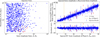 |
Fig. C.1 Summary of injection and recovery test to test the robustness of the FCO method in the limit of eight NEID observations obtained in three different visits. a) Period ratio between a hypothetical planet c and b as a function of the semi-amplitude ratio of the planets. Blue dots represent runs where the RV amplitude of planet b was successfully recovered (within 3σ of the injected value), while the red dots indicate nonrecovered runs. b) Recovered RV semi-amplitudes Kfit as a function of injected RV semi-amplitudes for planet b (top). Similarly to panel a, blue dots represent recovered runs, whereas red dots indicate nonrecovered runs, and the yellow vertical line indicates our adopted RV semi-amplitude of TOI-2431 b from Table 2. The 1–1 line is indicated with the black dashed line. We see that the recovered values are in good agreement with the injected values. |
All Tables
Derived parameters of TOI-2431 b from a joint analysis of available transit and RV data.
All Figures
|
Fig. 1 TESS target pixel file image of TOI-2431 in Sector 31. The electron fluxes are shown with the color bar. The red-bordered pixels highlight the pixels used for the PDCSAP light curve. The TESS pixel scale is approximately 21″. The size of the red circles indicates the TESS magnitudes of all nearby stars and TOI-2431 (white cross). Gray arrows show the proper motion directions of the stars in the field. |
| In the text | |
|
Fig. 2 Results from NESSI speckle imaging of TOI-2431. The plot shows the contrast curve as observed in the NESSI 562 nm filter (blue curve), and the 832 nm filter (red). The inset images highlight 256 × 256 insets of the reconstructed images. No secondary companions are seen. Note that in this figure, 1″corresponds to 36 AU at the distance of TOI-2431 b. |
| In the text | |
|
Fig. 3 Movement of TOI-2431 as a function of time. Left: POSS-I image of TOI-2431 (middle star) taken in 1954. Right: ZTF image of TOI-2431 taken in 2018. The red circle highlights the position of TOI-2431 as measured by Gaia at the Gaia J2016 epoch. Due to its high proper motion, TOI-2431 has moved substantially between the two images, highlighting that there is no background star seen in the vicinity of TOI-2431 that could confound the planet interpretation of TOI-2431 b. |
| In the text | |
|
Fig. 4 Best-fit results from a joint transit and RV fit using the FCO method for the RV data. a) Detrended TESS photometric observations (2 min exposures) are shown in blue at the top, folded on the time of transit. Best-fit transit model is shown in red. The black points show the TESS data binned to a cadence of 2 min. Residuals from the best-fit model are shown at the bottom. b) Phase-folded RV data and best-fit model (red) of TOI-2431 as observed with NEID in three separate visits listed as NEID1 (blue), NEID2 (yellow), and NEID3 (green), shown at the top. The red-shaded regions show the 1, 2, and 3σ credible intervals of the best-fitting model. Residuals from the best-fit model on the bottom. We adopted the values from this fit as the values for TOI-2431 b. |
| In the text | |
|
Fig. 5 Best fit results from a joint transit and RV fit using a quasi-periodic GP model to account for the excess RV scatter in the RVs. a) NEID (yellow) and HPF (green) RVs as a function of time at the top. The best-fit Keplerian model is shown in red (appears as a solid band due to the short period orbit). The median of the GP component is shown in blue. The joint best-fit model is shown in grey. Residuals from the best fit model, shown at the bottom. b) Phase-folded RVs on the period of TOI-2431 b, shown at the top. Best-fit Keplerian model after subtracting the GP model is in red. RV residuals as a function of phase are shown at the bottom. |
| In the text | |
|
Fig. 6 BLS periodogram of the TESS data. Top: BLS periodogram of all of the TESS sectors. The highest peak reveals the period of TOI-2431 b of 0.22 days, which is highlighted with the black dashed vertical line. Aliases of this period are also shown as faint dashed lines. The horizontal red dashed line shows a SDE of 10, the threshold we adopt for a significant signal. Bottom: BLS periodogram of the TESS data after masking out the transits of TOI-2431 b. No significant peaks are detected. |
| In the text | |
|
Fig. 7 GLS periodogram and window function of the NEID RVs of TOI-2431. a) GLS periodogram. The grey dotted line represents the FAP of 1%. The period of TOI-2431 b is highlighted with red vertical dashed line and the half-period is highlighted with blue vertical dashed line. Beyond the peak seen at Porb/2, we see no additional signals with a FAP< 1%. b) Window function of the RVs shown in panel a. |
| In the text | |
|
Fig. 8 Planet radius as a function of planet mass along with lines of constant density from (Zeng et al. 2019). The gray-shaded region indicates planets with iron content exceeding the maximum value predicted from models of collisional stripping (Marcus et al. 2010). Confirmed USP planets are shown with bold foreground points, and other confirmed exoplanets from the NASA Exoplanet Archive are shown with the faint purple points. TOI-2431 b is shown in red. We only show systems with better than 3σ mass and radius constraints. |
| In the text | |
|
Fig. 9 a) Expected tidal deformation of USPs parametrized as a (R1 − R3)/R1 as a function of Porb/PRoche. Here the planets are approximated as compressed ellipsoids with primary axes radii of R1, R2, and R3, where R1 is the radius of the planet pointing toward the star, and R3 is the radius along the orbit normal. We see that TOI-2431 b is among some of the most tidally distorted USP planets. b) Roche limit timescales of USPs as a function of Porb/PRoche. The latter indicates the proximity to the Roche limit, and the former indicates the timescale to reaching the Roche limit. We see that TOI-2431 b has the shortest timescale until tidal disruption of ~31 Myr. |
| In the text | |
|
Fig. 10 Planet radius as a function of orbital period for known exoplanets. Confirmed planets with a 3σ or higher precision mass detection are highlighted in blue. The planets that have a mass detection smaller than 3σ precision are shown in gray. TOI-2431 b is shown in red. TOI-2431 b is the shortest period planet with both a characterized mass and radius (better than 3σ). a) TOI-2431 b compared to other USPs. b) Same as panel a, but comparing TOI-2431 b to the broader exoplanet population showing that TOI-2431 b is at the lower edge of the hot Neptune desert. |
| In the text | |
|
Fig. 11 JWST Emission Spectroscopy Metric (ESM) (Kempton et al. 2018) as a function of planet orbital period for TOI-2431 b and other confirmed USP planets. TOI-2431 b is highlighted with the star, and other well-characterized USPs are shown with the thicker labels. The color bar shows the dayside equilibrium temperature assuming an albedo of AB = 0. |
| In the text | |
|
Fig. C.1 Summary of injection and recovery test to test the robustness of the FCO method in the limit of eight NEID observations obtained in three different visits. a) Period ratio between a hypothetical planet c and b as a function of the semi-amplitude ratio of the planets. Blue dots represent runs where the RV amplitude of planet b was successfully recovered (within 3σ of the injected value), while the red dots indicate nonrecovered runs. b) Recovered RV semi-amplitudes Kfit as a function of injected RV semi-amplitudes for planet b (top). Similarly to panel a, blue dots represent recovered runs, whereas red dots indicate nonrecovered runs, and the yellow vertical line indicates our adopted RV semi-amplitude of TOI-2431 b from Table 2. The 1–1 line is indicated with the black dashed line. We see that the recovered values are in good agreement with the injected values. |
| In the text | |
Current usage metrics show cumulative count of Article Views (full-text article views including HTML views, PDF and ePub downloads, according to the available data) and Abstracts Views on Vision4Press platform.
Data correspond to usage on the plateform after 2015. The current usage metrics is available 48-96 hours after online publication and is updated daily on week days.
Initial download of the metrics may take a while.