| Issue |
A&A
Volume 707, March 2026
|
|
|---|---|---|
| Article Number | A354 | |
| Number of page(s) | 17 | |
| Section | Extragalactic astronomy | |
| DOI | https://doi.org/10.1051/0004-6361/202556535 | |
| Published online | 18 March 2026 | |
Ultra-diffuse galaxies in the Kilo-Degree Survey with deep learning
1
Department of Physics “E. Pancini”, University of Naples Federico II, Via Cintia, 21, 80126 Naples, Italy
2
School of Mechanical, Electrical and Information Engineering, Shandong University, 180 Wenhua Xilu, Weihai 264209, Shandong, China
3
Institute for Astrophysics, School of Physics, Zhengzhou University, Zhengzhou 450001, PR China
4
INAF – Osservatorio Astronomico di Capodimonte, Salita Moiariello 16, I-80131 Napoli, Italy
5
INFN, Sez. di Napoli, via Cintia, 80126 Napoli, Italy
6
INAF – Osservatorio Astronomico di Capodimonte, Salita Moiariello 16, I-80131 Napoli, Italy
7
School of Mathematics and Physics, Xi’an Jiaotong-Liverpool University, 111 Renai Road, Suzhou 215123, PR China
8
INAF – Osservatorio Astronomico di Padova, vicolo dell’Osservatorio 5, I-35122 Padova, Italy
9
Ruhr University Bochum, Faculty of Physics and Astronomy, Astronomical Institute (AIRUB), German Centre for Cosmological Lensing, 44780 Bochum, Germany
10
School of Physics and Astronomy, Sun Yat-sen University, Zhuhai Campus, 2 Daxue Road, Xiangzhou District, Zhuhai 519082, China
11
Leiden Observatory, Leiden University, Niels Bohrweg 2, 2333 CA, Leiden, The Netherlands
12
School of Astronomy and Space Science, University of Chinese Academy of Sciences, Beijing 100049, China
13
INAF – Osservatorio Astronomico di Capodimonte, Salita Moiariello 16, I-80131 Napoli, Italy
★ Corresponding authors: This email address is being protected from spambots. You need JavaScript enabled to view it.
; This email address is being protected from spambots. You need JavaScript enabled to view it.
Received:
22
July
2025
Accepted:
24
December
2025
Abstract
Ultra-diffuse galaxies (UDGs) are a subset of low-surface-brightness galaxies (LSBGs), showing mean effective surface brightness fainter than 24 mag arcsec−2 and a diffuse morphology, with effective radii larger than 1.5 kpc. Due to their elusiveness, using traditional methods over large sky areas is challenging. Here we present a catalog of UDG candidates identified in the full 1350 deg2 area of the Kilo-Degree Survey (KiDS) using deep learning. In particular, we used a previously developed network for the detection of low-surface-brightness systems in the Sloan Digital Sky Survey (SBGnet) and optimized for UDG detection. We trained this new UDG detection network for KiDS (UDGnet-K), with an iterative approach, starting from a small-scale training sample. After training and validation, the UGDnet-K has been able to identify ∼3300 UDG candidates, of which, after visual inspection, we selected 545 high-quality ones. The catalog contains the independent rediscovery of previously confirmed UDGs in local groups and clusters (e.g., NGC 5846 and Fornax), and new discovered candidates in about 15 local systems, for a total of 67 bona fide associations. Besides the value of the catalog per se for future studies of UDG properties, this work shows the effectiveness of an iterative approach to training deep learning tools in presence of poor training samples, due to the paucity of confirmed UDG examples, which we expect to replicate for upcoming all-sky surveys such as those by the Rubin Observatory, Euclid, and the China Space Station Telescope.
Key words: catalogs / galaxies: dwarf / galaxies: structure
© The Authors 2026
 Open Access article, published by EDP Sciences, under the terms of the Creative Commons Attribution License (https://creativecommons.org/licenses/by/4.0), which permits unrestricted use, distribution, and reproduction in any medium, provided the original work is properly cited.
This article is published in open access under the Subscribe to Open model. This email address is being protected from spambots. You need JavaScript enabled to view it. to support open access publication.
1. Introduction
With extraordinary advances in deep, high-resolution imaging surveys over the past decades, an increasing number of ground-based and space programs have been started (e.g., Euclid, Laureijs et al. 2011; Amendola et al. 2018, the Dark Energy Survey – DES, Sevilla-Noarbe et al. 2021) or are approaching operations (e.g., Rubin Observatory/LSST, Abell et al. 2009, the China Space Station telescope – CSST, Zhan 2011; Gong et al. 2019). These facilities will provide unprecedented survey depths and image quality, enabling the detection of more numerous and fainter astronomical objects, as well as pushing forward the investigation of the low-surface-brightness side of galaxies. Low-surface-brightness galaxies (LSBGs) have been studied in great detail for decades (Impey et al. 1988; De Blok & McGaugh 1997; Hayward et al. 2005; Du et al. 2015; Greco et al. 2018; Tanoglidis et al. 2021). Detailed investigations of their properties have drawn attention to a seemingly distinct subclass of ultra-diffuse galaxies (UDGs), originally identified in the Coma cluster (e.g., Van Dokkum et al. 2015).
The UDGs are extended LSBGs, with g-band central surface brightnesses μ0(g)≥24 mag arcsec−2 and Milky Way-like effective radii Re ≥ 1.5 kpc (Van Dokkum et al. 2015), but stellar masses ∼102 to 103 times smaller than the Milky Way, making them comparable to dwarf galaxies. The UDG-like galaxies had already been identified in the 1980s (e.g., Sandage & Binggeli 1984), but the term “UDG” itself was only coined later by Van Dokkum et al. (2015). Since their postulation and first characterization, they have been regularly searched for in deep imaging data (van Der Burg et al. 2017), although searches have been mostly concentrated in galaxy clusters, such as the Hydra cluster (La Marca et al. 2022). For instance, the Coma cluster alone was found to have ∼103 UDGs (Koda et al. 2015; Yagi et al. 2016; Zaritsky et al. 2018; Alabi et al. 2020). Other studies have targeted Virgo (Mihos et al. 2016; Boselli et al. 2016; Lim et al. 2020), Fornax (Venhola et al. 2018), Hydra (Iodice et al. 2020), Perseus (Wittmann et al. 2017; Gannon et al. 2022; Marleau et al. 2024), Abell 2744 (Lee et al. 2017), and Abell 168 clusters (Román & Trujillo 2017a), suggesting that UDGs constitute a common population in high-density environments. However, UDGs have also been found to populate galaxy groups (Merritt et al. 2016; Román & Trujillo 2017b; Bennet et al. 2017) and the field (Bellazzini et al. 2017; Prole et al. 2019a; Leisman et al. 2017; Borlaff et al. 2022; Euclid Collaboration: Marleau et al. 2026).
Despite their ubiquity, and the systematic studies, including spectroscopy (see e.g., Chilingarian et al. 2019; Gannon et al. 2024), their origin and evolution history remains elusive. Understanding why they are such strong outliers in the typical galaxy scaling relations (especially μe − Re, Román & Trujillo 2017a) is therefore important (Amorisco & Loeb 2016; Bautista et al. 2023).
One possibility is that UDG formation is driven by external processes, with the star formation in these “failed” galaxies having been rapidly quenched at high redshift due to environmental processes in galaxy clusters (Koda et al. 2015; Yozin & Bekki 2015). If so, they should be dominated by dark matter, as it seems to be suggested by the large number of globular clusters (GCs) in these systems (see e.g., Saifollahi et al. 2022). In other scenarios, they are disks transformed by the interaction with dense environments (e.g., Tremmel et al. 2020), leaving the signature in their morphology (low axis ratio, low Sérsic index) or stellar population (old age, short-lived star formation). Supporting this scenario, large UDGs have been associated with tidal material and interaction with companion systems (Toloba et al. 2015; Bennet et al. 2018). On the other hand, internal processes, such as strong stellar feedback and gas outflows, may have dominated the formation of UDGs in isolated environments, leading to their diffuse stellar distributions (Tremmel et al. 2020). Finally, UDGs may be “genuine” dwarf galaxies with standard halo mass and luminosity, but anomalously large sizes, which could arise if they inhabit dark matter haloes with unusually large spin parameters (Amorisco & Loeb 2016), or from feedback and outflows that expand both the dark matter and stellar components of dwarf galaxies (Di Cintio et al. 2024), as is possibly suggested by the presence of color gradients (Liu et al. 2017).
It is important to better characterize UDGs for their mass content. Although there are limited works directly measuring their dynamical mass, most UDGs are inferred to be dark-matter-dominated, in some cases showing dark matter fractions of up to 98% (Koda et al. 2015). Thus, depending on the effective abundance of UDGs, they can contribute with a significant fraction of the measured dark matter in the Universe. For all these reasons, it is essential to collect larger samples of these systems to fully characterize their structure and internal dynamics as a function of the environment in which they live. Large sky surveys are the natural datasets to collect and explore large samples of them. Bennet et al. (2017) developed a new detection algorithm, specifically designed for modern wide field imaging surveys, and found 38 unreported diffuse dwarf candidates, of which seven may be UDG candidates. As was mentioned previously, the UDG class is a subset of the LSBG, which means they can be identified within existing LSBG collections (Yagi et al. 2016). However, among all the selection methods, the traditional procedures for detecting UDGs usually involve softwares such as Sextractor (Bertin & Arnouts 1996) or MTO (Teeninga et al. 2016) to extract sources from images, identifying their RA and Dec. Subsequently, other softwares, such as GALFITM (Peng et al. 2002) or IMFIT (Erwin 2015), have been employed to fit their relevant photometric parameters (e.g., their effective radius and mean effective surface brightness), which have been used to select candidates. From these, the final sample selection is confirmed via visual inspection (Van Dokkum et al. 2015; Yagi et al. 2016; Alabi et al. 2020; Bautista et al. 2023).
Although traditional methods have yielded certain results, they still have limitations. The primary challenge is that these methods are not specifically designed for identifying UDGs; hence, they extract all sources and from the measurement of the structural parameters they can isolate UDGs. This poses two levels of problems. First, current and future surveys will detect a number of sources that can be on the order of billions. Thus, extracting and fitting parameters to all these sources would take immense time and resources. Second, due to the low brightness and diffuse morphology of UDGs, uncertainties on structural parameters can be large and using solely them as a criterion to select UDGs can produce incomplete collections, as candidates can be lost due to the scatter of the size and surface brightness measurements (He et al. 2020; Yi et al. 2022). This would make the detection of these galaxies highly inefficient and time-consuming on vast data volumes such as the ones collected from Stage III surveys such as the Dark Energy Survey (DES, Sevilla-Noarbe et al. 2021), the Kilo-Degree Survey (KiDS, de Jong et al. 2013), and future Stage IV surveys such as the Legacy Survey of Space and Time (LSST, Ivezić et al. 2019), Euclid Mission (Euclid Collaboration: Aussel et al. 2026), the VLT Survey Telescope Survey of Mass Assembly and Structural Hierarchy (VST-SMASH, Tortora et al. 2024), and the CSST (Cao et al. 2018).
To overcome these challenges, there has been a growing effort to employ deep learning approaches for the detection of UDGs in wide-field surveys. For example, Tanoglidis et al. (2021) applied convolutional neural networks to DES data to search for LSB galaxies, while more recent works extended these techniques to other surveys such as HSC and UNIONS (Thuruthipilly et al. 2025; Heesters et al. 2025). Additionally, Yi et al. (2022) developed the LSBG-AD model, which utilized deep learning for the automatic detection of LSB galaxies from SDSS images. Their model detected 1 197 LSB galaxy candidates, including 116 new discoveries, demonstrating the potential of deep learning in uncovering previously unidentified faint galaxies. These studies collectively demonstrate the capability of deep learning models to efficiently and reliably identify faint and extended systems across massive imaging datasets, highlighting the pressing need for developing end-to-end, automated, and reliable methods for large-scale UDG detections in large datasets, with the goal of minimizing the number of candidates over which detailed structural parameter analyses must be performed. In this work, our primary aim is to introduce a novel deep-learning-based method of UDG detection, specifically designed for high-quality (HQ), multicolor, ground-based imaging data, and to present a first deep-learning-based catalog of HQ UDG candidates in KiDS.
In a previous work (Su et al. 2024), we introduced a framework for detecting LSBGs, called LSBGnet. This is based on a “you only look once” (YOLO) object detection model (Redmon 2016), previously used for object detections in astronomical images (Grishin et al. 2023), including LSBGs (González et al. 2018). The network architecture and image processing methods have been adjusted according to the characteristics of LSBGs, including the incorporation of the coordinate attention (CA) mechanism (Hou et al. 2021), gamut transformation, and mosaic data augmentation. In our first application, we built the LSBGnet-SDSS model and LSBGnet-DES model using datasets from the Sloan Digital Sky Survey (SDSS) and DES, respectively. These models achieve over 97% recall and precision on the test sets, demonstrating an excellent performance of the framework for LSBGs’ detection (Su et al. 2024). Due to the flexibility of this tool, we want to specialize the LSBGnet to the detection of UDGs. This new UDG detection network, or UDGnet for short, needs to be trained on real UDG images. In this paper, we present the results of a UDGnet model trained with UDGs from the KiDS fifth “Legacy” data release (Wright et al. 2024), which we dub UDGnet-K.
The first challenge facing us is building up an ad hoc training sample to train the tool for the systematic application to the whole KiDS dataset. Indeed, only a few UDGs are known in KiDS data from van Der Burg et al. (2017), which has performed a systematic detection for UDGs in a selected sample of galaxy groups, in 197 deg2 covered by Galaxy and Mass Assembly (GAMA, Driver et al. 2011)1. Hence, any training sample one can assemble will be necessarily smaller than standard samples usually adopted for training deep learning methods (i.e., convolutional neural networks – CNNs). Thus, we first focus on finding a strategy to enhance the training process, starting from a small training set, and then we effectively and accurately perform a first selection of the UDG candidates in the full KiDS DR5, covering an area of 1350 deg2 area (Wright et al. 2024).
For this specific work, we are not interested in fully quantifying the photometric properties of these candidates via surface brightness modeling, as the main purpose is to provide an automated method of robustly identifying UDGs in imaging data. Visual inspection of expert observers is the main step to score the quality of the deep learning detection. However, we still produce some realistic structural quantities to validate and check for visual biases.
This paper is organized as follows. In Sect. 2, we describe the KiDS data and the processing of the dataset. In Sect. 3, we illustrate the detection process of UDG candidates. In Sect. 4, we present the specific detection procedure and the corresponding results. Section 5 focuses on further filtering of the detected candidates to obtain the HQ sample and an analysis of their spatial distribution. Finally, in Sect. 6, we summarize our work and draw the conclusions.
2. Data
KiDS is a Stage III optical wide-field imaging survey (De Jong et al. 2017), carried out at the VST telescope (Capaccioli & Schipani 2011) with the OmegaCAM camera (Kuijken 2011), located at the European Southern Observatory (ESO), Cerro Paranal Observatory, in Chile. The final Data Release 5 (DR5) of the full area of ∼1350 deg2, observed in four optical filters (ugri), reaches a 5σ depth of r ∼ 24.8 mag, defined as the limiting magnitude measured in a 2″ diameter aperture (Wright et al. 2024). In DR5, as was done in previous releases, the optical imaging from VST has been combined with near-infrared (NIR) data of the VISTA Kilo degree Infrared Galaxy (VIKING, Edge et al. 2013; Venemans et al. 2015), which has observed the same KiDS area in ZYJHK using the Visible and Infrared Survey Telescope for Astronomy (VISTA), also located in Cerro Paranal. Total KiDS-DR5 then provides a unique 9-band multicolor dataset. Being primarily designed to map the large-scale distribution of matter in the Universe via weak lensing, KiDS is characterized by a very high image quality, with a point spread function (PSF) full width at half maximum (FWHM) of ∼0.7″ in the r band. Combined with the dark skies of Paranal, this makes the KiDS data ideal for low-surface-brightness studies (Roy et al. 2018; Kelvin et al. 2018).
In this paper, we intend to search for UDG candidates using gri-band composite images, consisting of large cutouts, or “chunks”, of the sky. The color images were generated with the HumVI2 package, adopting relative scalings of (0.4, 0.6, 1.7) for the g, r, and i bands, respectively, and using Q = 1.6 and α = 0.06 as the asinh stretch parameters. To ensure compatibility with the input dimensions of the UDGnet framework, we used chunks of 1001×1001 pixels, corresponding to a field of view of approximately 3.33’ at a pixel scale of 0.2 arcsec/pixel. An example of a sky chunk with a UDG candidate on top is shown in Fig. 1. Given the large effective radii of UDGs, to minimize mis-detections due to being too close to the edge of a sky chunk, we set a 100 pixel (∼20″) overlap of the different chunks. After the “cutting out” process, we obtained a total of 592 620 images completely covering the full KiDS area.
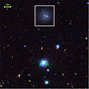 |
Fig. 1. Gri composite KiDS image with the white box highlighting a UDG candidate detected in the initial sample. |
As we intend to use a deep learning-based object detection algorithm (see Sect. 3), this requires us to provide not only the class of the objects, but also their location and size, indicated by a bounding box. In this work, we used LabelImg software (Tzutalin 2015) to manually label the UDG objects.
3. Methods
In this section, we illustrate the deep learning model adopted to obtain the detection of the best UDG candidates. The iterative process is implemented by augmenting the training sample, based on the step-by-step UDG detection, until the training sample has reached a sufficient size to proceed to the final selection of the best UDG candidates. We also introduce the definition of the structural parameters that is used to photometrically characterize the UDG candidates.
3.1. The UDG detection model (UDGnet)
As was mentioned, the UDGnet is based on the previously developed LSBGnet framework. The LSBGnet framework consists of four main steps: 1) image data augmentation; 2) building a LSBG detection network; 3) defining a loss function; 4) optimizing the network parameters and improving the model performance through iterative learning. Here, we did not update the detection network; we modified the image data augmentation based on the characteristics of the training images and UDGs. Additionally, we employed an iterative detection training strategy to build the model in the subsequent process.
The philosophy behind the UDGnet, equally to the original LSBGnet, is data-driven, and thus the characteristics of the training data largely determine the final detection performance of the model. Specifically, the images in the training set first underwent built-in data augmentation. This consists of scaling, flipping, color gamut transformation, and mosaic data augmentation. The augmented images are overlaid onto a 1024 × 1024 pixels gray-scale image before being input into the model. In our previous work, most galaxy samples were located centrally within images, which increased the risk of overfitting and decreased model robustness. To address this, we incorporated the enhancement of the mosaic data to improve the generalization of the model (Su et al. 2024). In this study, the dataset used does not suffer from the issue of objects being predominantly centered in the images. To streamline the training process and reduce computational overhead, we limited the proportion of mosaic data augmentation to 10% in the UDGnet framework. We also modified the range of scaling and gamut transformation data augmentation to ensure that the augmented images better align with the characteristics of UDGs.
3.2. The UDGnet for KiDS (UDGnet-K)
Finally, the new UDGnet also differs from the previous LSBGnet for the training set, which needs to be built on a specific HQ candidates, preserving the same noise, depth, and image quality of the images we need to use for the detection. Here, we present the strategy adopted for the UDGnet-K, trained on KiDS images. As was anticipated, the UDGnet training is based on an iterative approach. This starts with the initial step of building up the training set, beginning with a small initial sample of UDG candidates obtained through visual inspection by two researchers. We randomly selected approximately 30 noncontiguous tiles, covering a total area of about 30 deg2 from the KiDS survey, comprising 15 000 images. From these, we identified a sample of 35 UDG candidates, some of which are shown in Fig. 2. Among them, five sources had already been reported in Zaritsky et al. (2023). Looking at the sample in Fig. 2, we see that the main qualitative criterion in the UDG visual selection is the uniform light distribution with little or no substructure. In the first place, we excluded LSB systems with plumes or knots, because such substructures are not usually seen in UDG candidates, except possibly in the field (see e.g., Prole et al. 2019a). We shall discuss the impact of this choice later. For the moment, we remark that if, on the one hand, regular and smooth profiles represent the majority of the confirmed UDGs (see e.g., Román & Trujillo 2017b; Koda et al. 2015), on the other hand, this does not imply that the UDGnet will select only such systems, as the presence of background systems can still mimic the presence of substructures in the training sample.
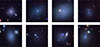 |
Fig. 2. Images of some UDG candidates in the training set. The size of each image is 40″ × 40″. Some UDG candidates appear off-center due to their positions being close to the borders of the image chunks. |
3.3. Structural parameters
To characterize the candidates identified by the UDGnet-K model, we need to compute their surface brightness and effective radius. As was mentioned earlier, in this paper we do not perform a full surface brightness fitting; for example, using a Sérsic profile (see van Der Burg et al. 2017). However, we introduce a simpler estimate of the effective radius, Re, and the brightness of the mean effective surface, ⟨μe⟩r, based on the luminosity growth curve in the r band. We use the r band because this is the highest-quality band in KiDS (FWHM ∼ 0.7″, see Kuijken et al. 2019); hence, we expect this to provide more unbiased estimates of the structural parameters in which we are interested. As was anticipated, we stress here that the seeing of the r-band images is smaller than the smallest effective radii we consider for the UDG candidates (i.e. 2″, see Sect. 3.3.1); hence, we expect the seeing to lightly affect the Re inferences, especially for large-angular systems. Finally, since we use r band instead of the canonical g band used to characterize the UDGs, we adopt a different standard for the UDG definition based on the mean surface brightness in the r band of ⟨μe⟩r ≥ 24 mag/arcsec2, widely used in literature (van Der Burg et al. 2017; Pina et al. 2019).
Before we detail the measurement of structural parameters, we stress that while the surface brightness is a distance-independent quantity and can directly be used to characterize the “diffuseness” of the candidates, the Re needs a distance to be converted on the linear scale from the angular scale is measured on the images. As we detail later (see Sect. 5.2), even if the UDGnet-K candidates have correspondent sources in the KiDS catalogs, their photometry is expected to be highly uncertain due to the intrinsically low surface brightness of these systems, making the publicly released photometric redshifts unreliable (de Jong et al. 2015). Moreover, these objects are expected to lie at low redshift (likely z < 0.1), a regime where photometric redshifts are generally less precise, further limiting their utility for accurate distance determinations.
3.3.1. Effective radius
For the measurement of the effective radius, we started by adjusting the bounding boxes predicted by the UDGnet-K model to ensure they completely encompassed the UDG candidates, including their surrounding diffuse halos. Next, due to the presence of field stars and galaxies overlapping with the surface brightness extension of the UDGs, we built a mask to exclude all pixels with fluxes exceeding ten times the average flux within the adjusted bounding box region. After masking these bright objects, we calculated the cumulative luminosity within circular areas with increasing values of their radii, L(< R). Importantly, we avoided using the outer regions where the growth curve flattens, as these areas may be affected by background over-subtraction that could lead to systematic underestimation of Re. To ensure a robust measurement, we instead derived Re from a parametric fit to the inner, well-constrained portion of the growth curve. We modeled the luminosity growth using a double-exponential function. First, we converted the surface brightness profile, μ(R), into linear intensity units (erg/s/cm2/Å):
 (1)
(1)
where the 10−7 term normalizes the flux scale. The growth curve was then fit with
 (2)
(2)
Here Lmax represents the asymptotic total luminosity, k controls the steepness of the curve, and R0 marks the transition radius where the growth rate changes. This functional form provides a flexible fit to the observed profile, while minimizing sensitivity to noise in the outskirts. The effective radius, Re, was derived from the best-fit model, corresponding to the radius enclosing half of Lmax, and the best-fit curve is shown in Fig. 3. Although growth-curve estimates may in principle overestimate Re when extrapolated, our comparison with literature GALFIT-based measurements for 21 UDGs (see 5.3) shows no significant systematic bias. In Fig. 4, we show the distribution of the derived Re for the visual sample of 35 UDGs, discussed in Sect. 3.1. As we can see they are mostly distributed in the range of 3 − 15 arcsec, consistently with what was found by van Der Burg et al. (2017). However, systematic studies of UDG candidates (e.g., Zaritsky et al. 2023) have found even broader effective radius distributions, reaching Re = 20″. In the following, we use the range 3 − 20 arcsec as a fiducial interval for realistic UDGnet candidate sizes. Typical errors on the estimate of these effective radii have been evaluated by varying the upper data point to be used to fit the growth curve before reaching the plateau. By perturbing this upper limit, we have found the effective radius estimates to vary up to ±0.05dex in log Re.
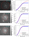 |
Fig. 3. “Growth curve” for a UDG candidate. In each of the left panels, the red circle represents the effective radius determined as the radius that encloses half of the total light, obtained by the growth curve in the right panel. The masks applied to exclude the brightest background and foreground objects are also shown in the left columns. The first row shows a known UDG candidate in the NGC 5846 galaxy group. |
It is worth noting that in our analysis we used circular annuli to construct the growth curves, to ensure a uniform methodology across the sample, and to avoid uncertainties from fitting position angles and ellipticities, which are often poorly constrained for very diffuse galaxies. However, for lower axis ratios, the use of circular rather than elliptical annuli can lead to a systematic underestimation of (Re), as the flux distribution along the minor axis is not fully captured (see, e.g., Yagi et al. 2016; van Der Burg et al. 2016). Since the majority of our candidates exhibit moderate-to-high axis ratios, this effect has a limited impact on the overall statistical properties of the sample. We acknowledge, though, that adopting elliptical apertures will better capture the intrinsic geometry of highly elongated sources, and we plan to implement this refinement in future analyses.
3.3.2. Effective surface brightness
For a galaxy to be defined as a UDG, we adopted a lower mean surface brightness of ⟨μe⟩r ≥ 24 mag arcsec−2. The r-band ⟨μe⟩, or μe for brevity, is defined as
 (3)
(3)
where Fluxe is defined as Fluxe = L(< Re)/πRe2, where L(< Re) is the total r-band luminosity3 within the effective radius, Re, obtained from the growth curve, L(< R), as in Sect. 3.3.1, and πRe2 is the area enclosed by Re.
As for the effective radii, by changing the fitting upper limit of the growth curve, we also estimated the typical error on ⟨μe⟩r and found it to be on the order of 0.2 mag/arcsec2. To account for these errors and minimize the lost of good candidates that might fall out of the definition because of errors on ⟨μe⟩r, we decided to finally adopt a lower conservative limit of ⟨μe⟩r > 23.8 mag/arcsec2. In the right panel of Fig. 4, we show the distribution of the ⟨μe⟩r of the visual sample of 35 UDGs. We see that most of the estimated μe are indeed compatible with the r-band 23.8 mag/arcsec2 as a lower limit for being UDGs. Only four of them turn out to have ⟨μe⟩r < 23.8 mag/arcsec2, which we excluded to finally retain 31 objects with r-band ⟨μe⟩r > 23.8 mag/arcsec2.
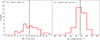 |
Fig. 4. Distribution of effective radius, Re, and mean effective surface brightness, ⟨μe⟩r, of the initial sample. The dashed black lines represent the median effective radius and mean effective surface brightness of the UDG candidates. |
3.3.3. Initial sample
Here, we summarize the properties of the initial sample to be used in the next steps of the UDGnet-K training, validation and results. This is the critical starting point as, depending on the criteria adopted, we might produce a biased UDG candidates’ catalog. This is made up of 31 candidates visually selected from a KiDS a randomly selected area of ∼30 deg2, whose properties are:
-
A growth curve circular effective radius in the range of 3″ < Re < 20″, consistently with Zaritsky et al. (2023);
-
An r-band mean effective surface brightness of ⟨μe⟩r > 23.8 mag/arcsec2, considering the typical error on growth curve.
4. Results
4.1. Sample expansion
The use of an adequate training sample is crucial for the UDGnet framework to effectively learn the features of the objects. To enable UDGnet-K to capture key characteristics, such as the morphology and brightness of the UDGs in the KiDS images, we used data augmentation to expand the initial sample obtained in Section 3.3.3.
To enlarge our training set, we applied three forms of data augmentation: scaling, flipping, and color–gamut transformations. Each original image was processed through a stochastic augmentation pipeline in which each transformation was applied with a probability of 0.5. As a result, objects did not necessarily undergo all augmentations. All augmented images were visually inspected, and those affected by artifacts or quality degradation were rejected. By iterating this procedure, we increased the initial sample of 31 UDGs to a final set of 100 HQ images, each containing a single UDG candidate. An example of the image appearance before and after data augmentation is illustrated in Fig. 5.
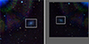 |
Fig. 5. Comparison of images before and after data augmentation. The panel on the left shows the original photometric image in the initial sample; the panel on the right shows the image after data augmentation. The white box indicates the UDG object. |
4.2. Iterative detection
We divided the augmented dataset into training, validation, and test sets in an 8: 1: 1 ratio, resulting in 80, 10, and 10 UDG candidates, respectively. The training set was utilized to train the model over 200 epochs. As was mentioned above, our UDGnet framework incorporates a data augmentation module. Except for the mosaic augmentation, the data augmentation strategies within the model are consistent with those applied during sample expansion. Therefore, during the initial training with the dataset described in Sect. 4.1, we set the in-model data augmentation rate to 10%. In subsequent iterative training stages, this rate was increased to 50%. It is important to note that the mosaic augmentation rate was consistently maintained at 10%.
After 200 training epochs the updated UDGnet-K model is considered fully trained, as is shown by the loss curve in Fig. 6. Using this model with a confidence threshold sets to 0.5, we identified a total of 19 UDG candidates within the 10 cutouts comprising the test set. Only 6 of the candidates correspond to the previously labeled UDG test samples, resulting in a recall rate of 60%. The visual inspection of the remaining candidates reveals that most of them possess a diffuse surface brightness distribution, typical of the appearance of UDGs. Four of these “newly discovered” UDG candidates are shown in Fig. 7. However, some others also show a rather irregular shape, including the presence of pseudo-arms, which is incompatible with them being canonical UDGs. We derived the μe and Re of all these new detections and they all show values within the UDG definition, which suggests that the structural parameters are not enough to define a UDG. Instead, only visual inspection can ensure the genuinity of the new UDG detections and the purity of the extended training set. Hence, in the following, we primarily use visual inspection to collect the training set, while we leave the structural parameters as the last selection criteria to adopt to refine the final UDG catalogs.
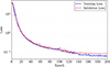 |
Fig. 6. Loss curves of training and validation. |
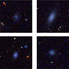 |
Fig. 7. Images of the four candidates detected in the first round test set of the iterative training set building-up. |
Going back to the training process, if, on the one hand, the discovery of new UDG candidates on top of the pre-selected test sample suggests that the model has learned the features of UDGs already at this step, on the other hand, the low recovery rate (60%) also suggests that the model has margins to be improved. To do that, we have implemented an iterative detection method, consisting of the following steps:
(1) Image grouping: the KiDS image catalog of 592,620 chunks (see Sect. 2) was split into four groups of 150k, 150k, 150k, and 142,62k chunks, respectively, according to their locations in the sky.
(2) Selection and detection: this step consists of applying the UDGnet-K model trained on the initial 100 UDG samples, to detect UDG candidates in the first group of 150k images.
(3) Visual inspection and labeling: This consists of visual inspection of newly detected UDG candidates, to add those that are correctly identified back to the initial set of augmented 100 UDG training and to obtain an expanded set of labeled training.
(4) Retraining: here we retrain the UDGnet-K model with the updated training set.
(5) Repeating: in this step we use the retrained UDGnet-K model to detect UDG candidates in the next group of images, and repeat the process from step (2) until the detection has been concluded in the last group of images.
This iterative detection method not only maximizes the utility of existing data but also facilitates the discovery of new UDG candidates, thereby providing a more comprehensive and diverse training set to enhance model training. After full round of training and detection, we had collected a total of 493 UDG candidates (excluding the data-augmented images), of which 77 had already been reported in Zaritsky et al. (2023).
4.3. Final sample selection
The expanded training set derived in the previous section was used to retrain the UDGnet-K model a last time, which was then applied to perform a final discovery run across all 592,620 chunks. To assess the performances of the tool we used the Recall, Precision and f1 score, defined as follows:
 (4)
(4)
 (5)
(5)
 (6)
(6)
where N is the number of known UDGs in datasets. Based on our final training results, we obtain a Precision of 90%, a Recall of 81%, and an F1 score of 85.2%.
In terms of computing time, to give a perspective, each full training session took approximately 3 hours, using an NVIDIA RTX 3070 GPU. On the other hand, the model prediction speed increases from 5 FPS when output images are produced, to 20 FPS without output images.
The fully trained UDGnet-K model detected 3,315 potential UDG candidates, although a quick check has shown the presence of bad images, some objects at the edge of the images, and duplicated candidates. After a cleaning check performed by two of us to delete all critical situations and outlier candidates (including irregular and LSB pseudo-spiral systems), and having also eliminated the duplicates found in the overlapping areas of contiguous chunks, we are left with a total of 966 candidates. By imposing the final criterion to their effective radius (3″ < Re < 20″) and mean effective surface brightness (⟨μe⟩r > 23.8 mag/arcsec2), we are finally left with 693 candidates. In Fig. 8 we show the distribution of the Re and μe, as compared to the 966 sample. We find that the majority of candidates exhibit effective radii concentrated in the range of 6″ to 10″, consistent with the size distribution of UDG populations reported in other large-scale detection efforts (e.g., Zaritsky et al. 2021). However, we also see a tail of objects with ⟨μe⟩r > 23.8 mag/arcsec2 and 10″ < Re < 15″ and only a few with Re > 15″, while there is a group of systems with Re > 20″. A visual inspection of these systems shows that the majority of them have a clear spiral-like structure, while there are four of them that still look like UDGs, with quite resolved stars in them, suggesting that they are very nearby systems. Assuming 1.5 kpc as the lower limit for UDGs, and a standard Planck Λ cold dark matter (CDM) cosmology (Aghanim et al. 2021), this implies that a lower redshift limit of would translate into a scale of 1.5kpc/21″ ∼ 0.075 kpc/arcsec, or a lower distance bound of 15 Mpc, almost equivalent to the Virgo Cluster. The median value of Re for our candidates is 7.7″, which, assuming, again, 1.5 kpc as the lower limit for UDGs, corresponds to a physical scale of 1.5/7.7 = 0.195 kpc arcsec−1. Under a standard Planck ΛCDM cosmology (Aghanim et al. 2021), this implies a lower redshift limit of z ∼ 0.01 (approximately 43.5 Mpc), suggesting that a large fraction of our UDG candidates are likely located in the nearby Universe (see Sect. 5.3 and 5.4). A random selection of the 693 UDG candidates is shown in Fig. 9, where they are separated according to their ⟨μe⟩r. Among these we still can see some dubious objects with irregular features, and residual of spiral arms. To select a HQ sample with minimal contamination from non-UDGs, we performed a full visual review of the 693 objects.
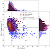 |
Fig. 8. Distribution of effective radius, Re, and mean effective surface brightness, ⟨μe⟩r, of UDG candidates. Blue circles: Full catalog of 966 candidates. Red circles: 693 candidates meeting the selection criteria (3″ < Re < 20″, ⟨μe⟩r > 23.8 mag/arcsec2). Black stars: 545 HQ Grade A candidates (see Sect. 5.1). Shaded density contours and axis histograms show the distributions of each sample. Dashed black lines indicate the median values of Re and ⟨μe⟩r. |
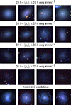 |
Fig. 9. Examples of candidates in different mean effective surface brightness ranges. Each row’s mean effective surface brightness falls within a specific range. In the last row, we show some non-UDG candidates. The size of each image is 30″ × 30″. |
Catalog of some HQ UDG candidates.
5. High-quality sample
In this section, we report the results of the grading of the 693 candidates. We reiterate that this sample was obtained from the original “potential” UDG candidates (3315) from the direct application of UDGnet-K, from which we derived a “cleaned” sample of 966 objects that reduced to 693 by imposing the adopted constraints on Re and ⟨μe⟩r. The ranking of this latter sample defines the HQ sample with which we study the spatial distribution across the KiDS area and derive some conclusions about their tentative environment.
5.1. Visual grading
The UDG candidate sample was graded by eight inspectors, who evaluated the color-combined images of the candidates. Each candidate was assigned to one of four grades, corresponding to scores indicated in brackets: a. a secure UDG (10), b. probably a UDG (7), c. probably not a UDG (3), d. a non-UDG (0).
The final score of each UDG candidate was obtained by averaging the score of the eight inspectors. These average values have been used to define an “average” grade (⟨Grade⟩) defined as: C for average scores of (0-3), B for (3-7), and A for (7-10). Hence, a ⟨Grade⟩= A object is an object for which all inspectors have given b-grade or higher, roughly speaking, or 6/8 have an a or b grade, with the majority being a. In Table 1 we show a subsample of the final catalog of 693 candidates, where we report the main information including the coordinates (RA and Dec), the mean effective surface brightness, ⟨μe⟩r, the effective radius, Re, the average score, and the related standard deviation, σ, and ⟨Grade⟩. Here, σ represents the standard deviation of the scores from the eight inspectors, reflecting the level of agreement among them, while ⟨Grade⟩ indicates the final grade assigned to each candidate based on the average score.
In this catalog, the number of UDG candidates in categories A, B, and C are 545, 127, and 21, respectively. Interestingly, in our sample, there is a residual minority of non-UDGs, meaning that the “cleaning” step effectively eliminated most of the spurious detections.
The overall morphological criteria adopted have been the regularity of the surface brightness distribution and the absence of major substructures. Additional factors considered were the presence of bright nearby sources and the level or structure of the background, both of which could reduce the confidence of the classification. We stress, however, that these visual criteria may introduce biases with respect to the general definition of UDGs, which should be primarily based on structural properties such as size and surface brightness. Indeed, as was pointed out by Prole et al. (2019a), field UDGs may exhibit irregular shapes and signatures of star formation, such as blue knots and bluer overall colors. In this respect, our visual inspection might have excluded some genuine UDGs by rejecting such “irregular” systems and possibly introducing spatial selection effects, if these latter are truly dominating the field regions. We acknowledge that this epistemological distinction represents a potential source of systematics.
To check this more quantitatively, in particular if the exclusion of clearly irregular systems has selected redder, more passive UDGs, we derived the color properties of the visually inspected sample. We then derived the g − r color distribution of the HQ candidates, via growth curve analysis of their g−band images. The color distribution, in Fig. 10, is approximately Gaussian, with a mean of 0.559 and a standard deviation of 0.163.
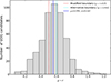 |
Fig. 10. Color distribution of HQ UDG candidates. The histogram shows the distribution of g − r colors, which is approximately Gaussian with a mean of 0.559 and a standard deviation of 0.163. The sample spans a broad range from blue to red systems without a pronounced bimodality. |
This is consistent with previous literature results on UDG colors, typically being smoothly distributed around similar g − r values (see e.g., Marleau et al. 2021 and Román & Trujillo 2017b), showing almost no difference with respect to non-UDG dwarf galaxies (see again Marleau et al. 2021). The inclusion of field UDGs usually shows weak bimodalities in UDG distributions (see also van Der Burg et al. 2016; Gannon et al. 2024); hence, we can conclude that our selection has captured the bulk of the UDG population, possibly missing a small fraction of bluer systems. We shall return to this point later.
The score distribution of the candidates is shown in Fig. 11, where we can see that more than half of the candidates, 270+118 = 388, have been judged as a sure UDG from almost all inspectors (average score larger than 9), while 28+106 = 134, have been judged to be sure UDG from about half of the inspectors (average score between 8 and 9). Overall, the A sample of 545 candidates can be considered a “golden” sample of HQ candidates4. A gallery of these HQ UDGs is shown in Fig. 12, where we also add four B and four C graded systems for comparison.
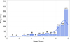 |
Fig. 11. Score distribution of UDG candidates. The histogram shows the number of sources at different score levels, while the blue curve represents the trend of the distribution. |
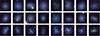 |
Fig. 12. Representative examples of UDG candidates by category (A, B, and C). In the first two rows, we show 16 UDG candidates of category A, and in the last row we show 4 candidates of category B and 4 candidates of category C. |
Looking into the details of the scoring, we find some correlations, which were partially expected. First, the lower the score, the larger the scatter among the inspectors, meaning that the visual definition of the UDG becomes more debated for unclear cases. For instance, almost all mean scores lower than 7 have a scatter larger than 2. By rechecking some of these objects, they all show substructures in their surface brightness distribution, such as knots or signatures of spiral arms (see Fig. 13). Although the presence of knots might still be consistent with the presence of star-forming regions mentioned earlier in this paper and in literature for field systems (see again Prole et al. 2019a), the presence of spiral-like structures or streams suggests that it is reasonable to discard those candidates. Hence, to conclude our epistemological note, we decided to maintain the conservative approach of excluding clearly irregular systems from our golden sample, accepting that this could reduce the completeness of our sample compared to other less conservative collections, but aiming to optimize the purity. For example, Prole et al. (2019a) claim the detection of ∼200 UDGs in 39 deg2 (or ∼5 UDG per deg2), which is almost a factor of 10 larger than our ∼550 UDGs in 1350 deg2 (i.e. ∼0.4 UDG per deg2). This factor is too large to be real, especially considering that the Prole et al. work refers to “field” candidates. We believe that this could be a consequence of the absence of any visual criteria to define a UDG sample, by looking at the example of UDG candidates in their paper. Also, fewer than half of their candidates would be qualified as HQ systems in our visual grading. To corroborate this conclusion, we notice that a sample of UDG candidates in low-to-moderate density fields from Marleau et al. (2021) have found, after a visual classification, 0.4 UDG/deg2.
We finally find that there is no correlation of the score with ⟨μe⟩r, except that the larger fraction of the low scores (< 7) reside in the brightest ⟨μe⟩r bin. Some of these objects are also shown in Fig. 13, where we can see that, even in this case, the objects show substructures and spiral-like structures that have driven the low grading.
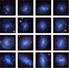 |
Fig. 13. UDG classification consistency and surface brightness properties. The top two rows show an increased disagreement (σ > 2) for lower-scoring candidates (mean score < 7). The bottom two rows show the candidates with low scores and a high surface brightness (⟨μe⟩r < 24 mag arcsec−2). |
5.2. Matching with the KiDS catalog
UDGs are objects that have intrinsically low signal-to-noise ratio (S/N), due to their diffuse light distribution. However, regardless of their intrinsic luminosity, they should be eventually detected in KiDS images from the detection pipeline (see e.g., de Jong et al. 2015), with only the lowest ones (see e.g., Fig. 9) being missed by the KiDS source lists. In order to check this for the HQ sample, we matched their coordinates with the KiDS-DR5 catalog (Wright et al. 2024). We used a matching radius of 2″, which is big enough to account for centroid errors, and small enough to minimize the mismatch with other background and foreground projected sources that can be close enough to the UDG centers (see e.g., Figs. 3 and 9). With this matching radius, we obtained 385/545 matches, i.e., 70% of the HQ sample. However, using a less conservative matching radius of 3″, we matched 465/545 HQ candidates, corresponding to about 85% of the full sample. It is very likely that a small fraction of the latter will indeed contain some mismatches; hence, for the following analysis, we considered the 2″ matched sample. In both cases, it seems clear that the UDG detection is possible even for standard general-purpose source extraction algorithms with no specific optimization for faint systems, but at the cost of a rather heavy incompleteness and contamination (see below). Indeed, the selection of UDG candidates in these catalogs should be based on the availability of reliable structural parameters that can be used to check the UDG criteria based on their size and surface brightness. For instance, in KiDS, besides multiband aperture and Kron photometry, no effective radii are provided in the released catalogs. Suitable parameters to identify UDGs from the KiDS catalogs are the mag_auto and the flux_radius from Sextractor (Bertin & Arnouts 1996) as a proxy of the total r-band magnitude and the circularized half-light radius, respectively. In the top panel of Fig. 14 we show that, if we consider the sources with mean S/N > 9, corresponding to mag_auto errors on the order of 0.33 mag, the mag_auto is well consistent with our total r-band magnitude estimate from the growth curve, with a mean difference of 0.12 ± 0.24 mag, i.e., slightly overestimating the magnitude although consistent with zero difference within 1σ. Below the S/N = 9, the mag_auto estimates start to become more scattered, as is shown in the bottom panel of Fig. 14 (red dots). In the same figure, we also show that the flux_radius parameter is a biased proxy of the effective radius, here represented by our estimate from the growth curve. In particular, a ∼20% underestimate of the Sextractor parameter is evident, consistent with the earlier finding of strong systematics affecting this parameter for LSB systems (e.g., Thuruthipilly et al. 2025).
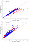 |
Fig. 14. Comparison of structural parameters (Mag and Re) between the HQ UDG candidates and their counterparts in the KiDS DR5 catalog. Top: The total r-band magnitudes derived from our growth curve method versus the KiDS catalog mag_auto values. Bottom: Re estimated from our growth curve compared with the KiDS catalog flux_radius. Red points indicate systems with large photometric uncertainties (> 0.33 mag). |
Therefore, blind searches based only on the use of standard catalog structural parameters are unreliable to select clean samples of UDG candidates. Indeed, underestimating the effective radii would cause the brightest ⟨μe⟩r, resulting in a loss of candidates. Also, should one rely on photometric parameters, a safe cut in the S/N would be needed to limit the contamination from noisy parameters. In this case, we have seen this would also produce the loss of relevant low-S/N candidates. Hence, the use of deep learning remains a viable and accurate alternative to the human visual search, to select complete samples of UDG candidates over large areas of the sky.
A final thing to mention is the photometric redshift. The KiDS DR5 catalog, as all previous releases, provides photometric redshifts from 9-band Gaussianized apertures, from the Bayesian photo-z software (BPZ, Benitez 2000). However, the accuracy of the publicly available BPZ photometric redshifts is not sufficient to make them useful for our weak-lensing analysis. In addition, as was already discussed in 3.3, BPZ photo-z estimates are particularly unreliable for UDGs due to their low surface brightness. In principle, we could use the same photo-z to associate a tentative distance to the matched UDG candidates with KiDS, as done for mag_auto and flux_radius. However, these errors are overwhelmingly higher than the true intrinsic redshift of these systems, especially if located at low redshifts (see Wright et al. 2024). To give a perspective, a UDG at z ∼ 0.05 (corresponding to ∼220 Mpc) would have a 100% error in redshifts, which more or less corresponds to a 100% error on the effective radius in kpc, making the use of photo-z basically pointless. For this reason, we decided to exclude the use of published photo-z in this analysis, hereafter.
5.3. Matching with external catalogs from literature
As a further validation of our catalog, in this section we report the results of the match of the HQ candidates listed in Table 1, with some external catalogs reported in the literature, which overlap with the KiDS footprint. In particular, we use local UDG samples from Venhola et al. (2017), Prole et al. (2019b), Marleau et al. (2021) and Zaritsky et al. (2023), which report candidates belonging to low redshift groups or clusters. The prominence of local candidates is not surprising as, due to the LSB nature of these systems, and intrinsic faintness, distance is a natural selection effect as for elusive systems, angular size helps the identification of convincing candidates, both for automatic searches (e.g., setting the number of pixels with a sufficient S/N as a criterion for a detection) and for visual inspections (where small LSB systems can be confused with correlated noise). We have also seen that more than half of our candidates have angular sizes that might be compatible with low redshifts (see Sect. 3.3), increasing the chance of selecting nearby systems.
Venhola et al. (2017, V+17 hereafter) have assembled a catalog of ∼200 LSBGs including 12 UDGs, which we have crossmatched with our HQ catalog. We have found two matches, of which only one candidate is classified as UDG in their catalog (FDS10_LSB52) – the other one (FDS11_LSB49) is slightly off the UDG range, being Re < 1.5 kpc within the errors. Indeed, a small scatter of the measurement around the 1.5 kpc threshold can make a standard LSBG to jump into the UDG sample, meaning that the classification of an object can change from dataset to dataset. In fact, this source (FDS11_LSB49) is classified as a UDG in the sample of Prole et al. (2019b), showing that small differences in the adopted threshold can affect the classification of some systems.
Assuming the same distance of Fornax of V+17, our matched systems all are confirmed to be UDGs, with Re = 1.81, 1.62 kpc and ⟨μe⟩r = 25.21, 24.35 mag/arcsec2, respectively. All the other V+17 candidates cannot be matched because they are distributed in the ∼3/4 of the cluster area, which is outside of the KiDS area. Interestingly, looking at the position on the sky of our HQ candidates (see also the next section), there are more UDG candidates in our catalog that might be associated with this cluster. Following the V+17 footprint, we checked which ones of the UDG candidates within 3 deg from the Fornax brightest cluster galaxy (BCG, NGC 1399) possess a Re > 1.4 kpc, assuming the same distance of the BCG. We used 1.4 kpc to account for the possibility that the UDG has a variation in the distance along the line of sight within the cluster. We found that five candidates (including the one already matched) are compatible with being UDG candidates of the Fornax cluster, three of which are new candidates missed in previous collections. All of the above information is reported in Table 2.
Crossmatch results of HQ UDG candidates with nearby clusters/groups.
The crossmatch with the MATLAS UDG catalog from Marleau et al. (2021), based on HST imaging, returned a total of seven matched candidates. Of these, they report two UDGs belonging to NGC 4690 and two around NGC 5576, all of which are recovered by our detection. We have also matched three of our UDG candidates with the catalog of five candidates associated with NGC 5846. In this case, the HQ catalog misses four objects that, on visual inspection, are too faint in KiDS with respect to the corresponding HST images. As for the Fornax cluster, we checked if other UDGs from our catalog are compatible with being associated with the same groups. In this case we used the galaxy distances to define a radius of 1 Mpc to select UDG candidates and convert the Re to kpc, again using 1.4 kpc as a lower limit to define the candidates as UDGs belonging to the group. As we report in Table 2, we found that three new UDGs are found in NGC 5576, three in NGC 4690, and two in NGC 5846.
Finally, we considered the recent SMUDGES UDG catalog from Zaritsky et al. (2023), from the Legacy Surveys (DECaLS, BASS, and MzLS). Their detection pipeline is based on a combination of surface brightness selection, size criteria, and careful visual inspection, yielding one of the largest compilations of UDG candidates to date, although they did not attempt to make any association with groups or clusters. In order to check the overlap with our finding, we applied our environmental association criteria to their catalog, i.e., we found their UDG candidates lying within a projected radius of 1 Mpc from the central galaxy and converted their effective radii into physical units using the corresponding group or cluster distances. We then crossmatched these candidates with our HQ catalog using a matching radius of 6″.
The results of this comparison are summarized in Table 2, where we find that several UDG candidates identified by Zaritsky et al. (2023) are also recovered in our catalog around specific clusters and groups. For the unmatched SMUDGES candidates, we conducted a careful inspection of their KiDS images and found that the vast majority are extremely faint, lying close to the surface-brightness limit of KiDS, which likely explains why they were not recovered by our deep-learning pipeline. The coordinates and main properties of these UDG members are reported in Appendix A.1.
To conclude this section, we can use the matched sample of 21 known UDGs (last column on the right in Table 2) for a sanity check of our structural parameters, by comparing the inferences of Re and magnitude (or Lmax) from Eq. 2 with the values reported in previous literature. We find δRe = RHQ − Rlit = −0.11 ± 0.15 (kpc), where RHQ is the effective radius from our catalog converted into kiloparsecs, assuming the associated group distance, and Rlit is the same radius from literature, and a δmr = mHQ − mlit = 0.08 ± 0.21 (mag), where mHQ is the r-band total magnitude from our catalog and the mlit is the same from the literature. ***Units should be written out in full when not following a numeral. Interestingly, both quantities show no systematic deviations within the statistical errors, even though our parameters are based on a less sophisticated procedure than the 2D surface fitting adopted in literature.
5.4. Spatial distribution and environment and associations in the local Universe
In the previous section, we saw that our HQ catalog contains matches with previously detected UDG candidates in the Fornax cluster, NGC4690, NGC 5846, and NGC 5576 groups. The KiDS footprint covers a large variety of environments, including many other close groups and clusters that we might expect the UDG candidates to be associated with. The distribution of the HQ candidates is illustrated in Fig. 15.
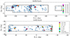 |
Fig. 15. Distribution of A-grade UDG candidates in KiDS DR5. The red crosses denote UDG candidates matched to known galaxy clusters. |
From this figure, we can see that the candidates are not uniformly distributed but seem to cluster in specific regions with locally higher number densities that generally fade into lower-density regions, very likely representing typical field environments. This suggests that the majority of UDGs are associated with overdensities tracing some large-scale structures. The great advantage of covering large areas of the sky is that KiDS can also provide many field UDGs, despite our selection criteria possibly having missed a fraction of irregular systems, as was discussed above. Keeping apart this possible incompleteness in the low-density areas, the UDGs inhabiting the high-density regions are more likely associated with nearby systems for which the distance is known. To check for these possible associations, we followed the same approach as in the previous section for the known UDGs, but using the catalog of bright nearby galaxies (i.e., absolute B-magnitude MB < −205). For each of these galaxies, we searched for the UDGs within a projected radius of 1 Mpc having a Re > 1.4 kpc, assuming for them the same distance as the large host galaxy. The results are shown in Table 2, where we report the ID of galaxies and clusters that are compatible with hosting UDGs and the number of them. These are also plotted in Fig. 15, where we see the nearby galaxies placing themselves in the center of the UDG overdensities, confirming the impression that a large fraction of UDGs have to be satellites of galaxies groups or clusters halos. In this work, we are not interested in a complete characterization of the environment of the UDG candidates, which we leave for a forthcoming paper. However, using the lesson learned in the previous section, it is important to assign an environment and a distance to a number of candidates in our catalog to have a confirmation of the nature of UDGs of these systems. As is seen in Table 2, we could associate only 67 UDG candidates because we have limited our choice to nearby systems (vrad < 8000 km/s), which matched almost all the high-density patches in Fig. 15. This number could be larger if we considered a larger area around them (i.e. larger than 1 Mpc), or if we checked further away groups or clusters. As a first attempt preluding a deeper and more attentive analysis of the environment for all the UDGs in the catalog, we just stress that we have an interesting first sample of UDG members in 15 nearby groups or clusters. Among these, in KiDS-North we remark a large concentration around the area connecting the NGC 5846 group and NGC 5576 group, which is worth being investigated in more detail, and the southern tails of the Virgo cluster (represented by NGC 4636), with an interesting filament extending toward NGC 4063. In the KiDS-South the quarter of the sphere around the center of the Fornax cluster is evident, as are other larger concentrations around NGC 7176, NGC 7507, and 2MASS-J22590127. The details of all the associated UDG candidates are again reported in Appendix A.1, together with the ones that have been found in the previous section.
6. Summary
In this paper, we have presented UDGnet, a new deep learning framework tailored for the large-scale detection of UDGs in photometric imaging data. This framework builds upon the previously proposed LSBGnet framework, which was originally developed for the identification of LSBGs. Based on UDGnet, we constructed a specialized model, UDGnet-K, specialized for application to the KiDS DR5 dataset. The direct application of the UDGnet-K to the full KiDS footprint, consisting of 1350 deg2, produced a sample of 3315 UDG candidates. After the removal of duplicate and spurious detections, we obtained a final sample of 966 objects. For all candidates we measured the effective radius, Re, and the mean effective surface brightness, ⟨μe⟩r, based on the luminosity growth curve in the images of the r- band, and selected UDG candidates based on reasonable selection criteria. The derived parameters exhibit no systematic deviations within the statistical uncertainties.
We opted for the selection threshold of ⟨μe⟩r ≥ 23.8 mag arcsec−2 and 3″ ≤ Re(r)≤20″. This brought us a catalog of 693 UDG candidates visually inspected by eight evaluators. We finally obtained HQ 545 UDG candidates, corresponding to a frequency of ∼0.4 UDG/deg2, consistent with other findings using visual inspection to obtain clean UDG samples.
The spatial distribution of UDG candidates across the KiDS footprint is rather inhomogeneous, with noticeable overdensities in some regions and others showing very few or no candidates per square degree. After crossmatching with existing catalogs of known local UDGs, we independently reidentified nine previously reported UDGs located in the Fornax cluster, as well as in NGC 5846 and NGC 5576 (see Table 2). In addition, we identified new UDG candidates within the same groups or clusters. This known sample has proven valuable for validating the robustness of our structural parameter measurements (Re and ⟨μe⟩r), which show excellent agreement – with negligible systematics – when compared to literature values, primarily derived using GALFIT.
We finally searched for more associations with nearby galaxy clusters, based on geometrical arguments, i.e., being within ∼1 Mpc of the group or cluster center and using the cluster redshift to select those objects whose Re > 1.5 kpc are at that redshift. This approach led to the identification of 67 new UDG candidates in several clusters, including the Fornax, ESO466-021, UGC 07813, and NGC groups, with a notably higher spatial number density compared to field regions, suggesting a strong environmental dependence for UDG occurrence. The full HQ catalog and the associations in the local Universe are provided in Tables 1 and 2, respectively.
The UDGnet-K model we developed inherits the advantages of the LSBGnet framework, which enables automated, end-to-end large-scale detection for LSBGs. Overall, the most labour–intensive part of our workflow is the construction of the initial training set. Once the network is trained, however, UDGnet-K can be applied in a fully automated way to much larger imaging datasets, with modest training and inference times.
Using KiDS DR5 as a test bench, we fully assessed a very effective iterative detection method allowing for large-scale detection of specific objects despite a lack of sufficient known samples, providing an effective approach for the subsequent detection of specific objects. These new UDGnets can be the foundation for models being developed for upcoming all-sky surveys such as those of the Rubin Observatory/LSST, Euclid, and the CSST.
Data availability
Table 1 is available at the CDS via https://cdsarc.cds.unistra.fr/viz-bin/cat/J/A+A/707/A354
Acknowledgments
This study was supported by the National Natural Science Foundation of China (NSFC) grant no 12573109. Rui Li acknowledges the support by the China Manned Space Program (no.CMS-CSST-2025-A03) and the National Natural Science Foundation of China (No. 12203050). NRN acknowledges support from the Guangdong Science Foundation grant (ID: 2022A1515012251). SH acknowledges the support of the China Scholarship Council (grant n. 202406220048). Rossella Ragusa acknowledges support grants through INAF-WEAVE StePS founds and through PRIN-MIUR 2020SKSTHZ. NRN acknowledges support from acknowledges support from the Guangdong Science Foundation grant (ID: 2022A1515012251). AHW is supported by the Deutsches Zentrum für Luft- und Raumfahrt (DLR), under project 50QE2305, made possible by the Bundesministerium für Wirtschaft und Klimaschutz, and acknowledges funding from the German Science Foundation DFG, via the Collaborative Research Center SFB1491 “Cosmic Interacting Matters – From Source to Signal”.
References
- Abell, P. A., Allison, J., Anderson, S. F., et al. 2009, [Google Scholar]
- Aghanim, N., Akrami, Y., Ashdown, M., et al. 2021, A&A, 652, 1 [Google Scholar]
- Alabi, A. B., Romanowsky, A. J., Forbes, D. A., Brodie, J. P., & Okabe, N. 2020, MNRAS, 496, 3182 [NASA ADS] [CrossRef] [Google Scholar]
- Amendola, L., Appleby, S., Avgoustidis, A., et al. 2018, Liv. Rev. Relat., 21, 1 [Google Scholar]
- Amorisco, N. C., & Loeb, A. 2016, MNRAS, 459, L51 [NASA ADS] [CrossRef] [Google Scholar]
- Bautista, J. M. G., Koda, J., Yagi, M., Komiyama, Y., & Yamanoi, H. 2023, ApJS, 267, 10 [NASA ADS] [CrossRef] [Google Scholar]
- Bellazzini, M., Belokurov, V., Magrini, L., et al. 2017, MNRAS, 467, 3751 [NASA ADS] [Google Scholar]
- Benitez, N. 2000, ApJ, 536, 571 [CrossRef] [Google Scholar]
- Bennet, P., Sand, D., Crnojević, D., et al. 2017, ApJ, 850, 109 [NASA ADS] [CrossRef] [Google Scholar]
- Bennet, P., Sand, D. J., Zaritsky, D., et al. 2018, ApJ, 866, L11 [NASA ADS] [CrossRef] [Google Scholar]
- Bertin, E., & Arnouts, S. 1996, A&AS, 117, 393 [NASA ADS] [CrossRef] [EDP Sciences] [Google Scholar]
- Borlaff, A. S., Gómez-Alvarez, P., Altieri, B., et al. 2022, A&A, 657, A92 [NASA ADS] [CrossRef] [EDP Sciences] [Google Scholar]
- Boselli, A., Cuillandre, J., Fossati, M., et al. 2016, A&A, 587, A68 [NASA ADS] [CrossRef] [EDP Sciences] [Google Scholar]
- Cao, Y., Gong, Y., Meng, X.-M., et al. 2018, MNRAS, 480, 2178 [Google Scholar]
- Capaccioli, M., & Schipani, P. 2011, Messenger, 146, 27 [Google Scholar]
- Chilingarian, I. V., Afanasiev, A. V., Grishin, K. A., Fabricant, D., & Moran, S. 2019, ApJ, 884, 79 [NASA ADS] [CrossRef] [Google Scholar]
- De Blok, W., & McGaugh, S. S. 1997, MNRAS, 290, 533 [NASA ADS] [CrossRef] [Google Scholar]
- de Jong, J. T., Verdoes Kleijn, G. A., Kuijken, K. H., et al. 2013, Exp. Astron., 35, 25 [NASA ADS] [CrossRef] [Google Scholar]
- de Jong, J. T., Kleijn, G. A. V., Boxhoorn, D. R., et al. 2015, A&A, 582, A62 [NASA ADS] [CrossRef] [EDP Sciences] [Google Scholar]
- De Jong, J. T., Kleijn, G. A. V., Erben, T., et al. 2017, A&A, 604, A134 [NASA ADS] [CrossRef] [EDP Sciences] [Google Scholar]
- Di Cintio, A., Arjona-Galvez, E., & Grand, R. 2024, EAS2024, 294 [Google Scholar]
- Driver, S. P., Hill, D. T., Kelvin, L. S., et al. 2011, MNRAS, 413, 971 [Google Scholar]
- Du, W., Wu, H., Lam, M. I., et al. 2015, AJ, 149, 199 [NASA ADS] [CrossRef] [Google Scholar]
- Edge, A., Sutherland, W., Kuijken, K., et al. 2013, Messenger, 154, 32 [Google Scholar]
- Erwin, P. 2015, ApJ, 799, 226 [Google Scholar]
- Euclid Collaboration (Aussel, H., et al.) 2026, A&A, accepted [arXiv:2503.15302] [Google Scholar]
- Euclid Collaboration (Marleau, F., et al.) 2026, A&A, in press, https://doi.org/10.1051/0004-6361/202554547 [Google Scholar]
- Forbes, D. A., Gannon, J., Couch, W. J., et al. 2019, A&A, 626, A66 [NASA ADS] [CrossRef] [EDP Sciences] [Google Scholar]
- Gannon, J. S., Forbes, D. A., Romanowsky, A. J., et al. 2022, MNRAS, 510, 946 [Google Scholar]
- Gannon, J. S., Ferré-Mateu, A., Forbes, D. A., et al. 2024, MNRAS, 531, 1856 [NASA ADS] [CrossRef] [Google Scholar]
- Gong, Y., Liu, X., Cao, Y., et al. 2019, ApJ, 883, 203 [NASA ADS] [CrossRef] [Google Scholar]
- González, R. E., Munoz, R. P., & Hernández, C. A. 2018, Astron. Comput., 25, 103 [CrossRef] [Google Scholar]
- Greco, J. P., Greene, J. E., Strauss, M. A., et al. 2018, ApJ, 857, 104 [NASA ADS] [CrossRef] [Google Scholar]
- Grishin, K., Mei, S., & Ilić, S. 2023, A&A, 677, A101 [NASA ADS] [CrossRef] [EDP Sciences] [Google Scholar]
- Hayward, C. C., Irwin, J., & Bregman, J. 2005, ApJ, 635, 827 [NASA ADS] [CrossRef] [Google Scholar]
- He, M., Wu, H., Du, W., et al. 2020, ApJS, 248, 33 [Google Scholar]
- Heesters, N., Chemaly, D., Müller, O., et al. 2025, A&A, 699, A232 [NASA ADS] [CrossRef] [EDP Sciences] [Google Scholar]
- Hou, Q., Zhou, D., & Feng, J. 2021, in Proceedings of the IEEE/CVF Conference on Computer Vision and Pattern Recognition, 13713 [Google Scholar]
- Impey, C., Bothun, G., & Malin, D. 1988, ApJ, 330, 634 [Google Scholar]
- Iodice, E., Cantiello, M., Hilker, M., et al. 2020, A&A, 642, A48 [EDP Sciences] [Google Scholar]
- Ivezić, Ž., Kahn, S. M., Tyson, J. A., et al. 2019, ApJ, 873, 111 [Google Scholar]
- Kelvin, L. S., Bremer, M. N., Phillipps, S., et al. 2018, MNRAS, 477, 4116 [NASA ADS] [CrossRef] [Google Scholar]
- Koda, J., Yagi, M., Yamanoi, H., & Komiyama, Y. 2015, ApJ, 807, L2 [NASA ADS] [CrossRef] [Google Scholar]
- Kuijken, K., et al. 2011, Messenger, 146 [Google Scholar]
- Kuijken, K., Heymans, C., Dvornik, A., et al. 2019, A&A, 625, A2 [NASA ADS] [CrossRef] [EDP Sciences] [Google Scholar]
- La Marca, A., Iodice, E., Cantiello, M., et al. 2022, A&A, 665, A105 [NASA ADS] [CrossRef] [EDP Sciences] [Google Scholar]
- Laureijs, R., Amiaux, J., Arduini, S., et al. 2011, arXiv e-prints [arXiv:1110.3193] [Google Scholar]
- Lee, M. G., Kang, J., Lee, J. H., & Jang, I. S. 2017, ApJ, 844, 157 [CrossRef] [Google Scholar]
- Leisman, L., Haynes, M. P., Janowiecki, S., et al. 2017, ApJ, 842, 133 [NASA ADS] [CrossRef] [Google Scholar]
- Lim, S., Côté, P., Peng, E. W., et al. 2020, ApJ, 899, 69 [CrossRef] [Google Scholar]
- Liu, F., Jiang, D., Faber, S. M., et al. 2017, ApJ, 844, L2 [Google Scholar]
- Marleau, F. R., Habas, R., Poulain, M., et al. 2021, A&A, 654, A105 [NASA ADS] [CrossRef] [EDP Sciences] [Google Scholar]
- Marleau, F. R., Duc, P.-A., Poulain, M., et al. 2024, A&A, 690, A339 [NASA ADS] [CrossRef] [EDP Sciences] [Google Scholar]
- Merritt, A., van Dokkum, P., Danieli, S., et al. 2016, ApJ, 833, 168 [NASA ADS] [CrossRef] [Google Scholar]
- Mihos, J. C., Harding, P., Feldmeier, J. J., et al. 2016, ApJ, 834, 16 [Google Scholar]
- Peng, C. Y., Ho, L. C., Impey, C. D., & Rix, H.-W. 2002, AJ, 124, 266 [Google Scholar]
- Pina, P. E. M., Fraternali, F., Adams, E. A., et al. 2019, ApJ, 883, L33 [CrossRef] [Google Scholar]
- Prole, D., van der Burg, R., Hilker, M., & Davies, J. 2019a, MNRAS, 488, 2143 [NASA ADS] [CrossRef] [Google Scholar]
- Prole, D. J., Hilker, M., van der Burg, R. F., et al. 2019b, MNRAS, 484, 4865 [Google Scholar]
- Redmon, J. 2016, in Proceedings of the IEEE Conference on Computer Vision and Pattern Recognition [Google Scholar]
- Román, J., & Trujillo, I. 2017a, MNRAS, 468, 703 [CrossRef] [Google Scholar]
- Román, J., & Trujillo, I. 2017b, MNRAS, 468, 4039 [Google Scholar]
- Roy, N., Napolitano, N. R., Barbera, F. L., et al. 2018, MNRAS, 480, 1057 [Google Scholar]
- Saifollahi, T., Zaritsky, D., Trujillo, I., et al. 2022, MNRAS, 511, 4633 [NASA ADS] [CrossRef] [Google Scholar]
- Sandage, A., & Binggeli, B. 1984, AJ, 89, 919 [Google Scholar]
- Sevilla-Noarbe, I., Bechtol, K., Kind, M. C., et al. 2021, ApJS, 254, 24 [NASA ADS] [CrossRef] [Google Scholar]
- Su, H., Yi, Z., Liang, Z., et al. 2024, MNRAS, 528, 873 [NASA ADS] [CrossRef] [Google Scholar]
- Tanoglidis, D., Drlica-Wagner, A., Wei, K., et al. 2021, ApJS, 252, 18 [Google Scholar]
- Teeninga, P., Moschini, U., Trager, S. C., & Wilkinson, M. H. 2016, Math. Morphol. Theory Appl., 1 [Google Scholar]
- Thuruthipilly, H., Junais, J., Koda, J., et al. 2025, A&A, 695, A106 [NASA ADS] [CrossRef] [EDP Sciences] [Google Scholar]
- Toloba, E., Sand, D. J., Spekkens, K., et al. 2015, ApJ, 816, L5 [NASA ADS] [CrossRef] [Google Scholar]
- Tortora, C., Ragusa, R., Gatto, M., et al. 2024, arXiv e-prints [arXiv:2411.09608] [Google Scholar]
- Tremmel, M., Wright, A. C., Brooks, A. M., et al. 2020, MNRAS, 497, 2786 [Google Scholar]
- Tzutalin, D. 2015, GitHub Repository, 6, 4 [Google Scholar]
- van Der Burg, R. F., Muzzin, A., & Hoekstra, H. 2016, A&A, 590, A20 [NASA ADS] [CrossRef] [EDP Sciences] [Google Scholar]
- van Der Burg, R. F., Hoekstra, H., Muzzin, A., et al. 2017, A&A, 607, A79 [NASA ADS] [CrossRef] [EDP Sciences] [Google Scholar]
- Van Dokkum, P. G., Abraham, R., Merritt, A., et al. 2015, ApJ, 798, L45 [NASA ADS] [CrossRef] [Google Scholar]
- Venemans, B., Verdoes Kleijn, G., Mwebaze, J., et al. 2015, MNRAS, 453, 2259 [Google Scholar]
- Venhola, A., Peletier, R., Laurikainen, E., et al. 2017, A&A, 608, A142 [NASA ADS] [CrossRef] [EDP Sciences] [Google Scholar]
- Venhola, A., Peletier, R., Laurikainen, E., et al. 2018, A&A, 620, A165 [NASA ADS] [CrossRef] [EDP Sciences] [Google Scholar]
- Wittmann, C., Lisker, T., Ambachew Tilahun, L., et al. 2017, MNRAS, 470, 1512 [Google Scholar]
- Wright, A. H., Kuijken, K., Hildebrandt, H., et al. 2024, A&A, 686, A170 [NASA ADS] [CrossRef] [EDP Sciences] [Google Scholar]
- Yagi, M., Koda, J., Komiyama, Y., & Yamanoi, H. 2016, ApJS, 225, 11 [CrossRef] [Google Scholar]
- Yi, Z., Li, J., Du, W., et al. 2022, MNRAS, 513, 3972 [NASA ADS] [CrossRef] [Google Scholar]
- Yozin, C., & Bekki, K. 2015, MNRAS, 452, 937 [NASA ADS] [CrossRef] [Google Scholar]
- Zaritsky, D., Donnerstein, R., Dey, A., et al. 2018, ApJS, 240, 1 [NASA ADS] [CrossRef] [Google Scholar]
- Zaritsky, D., Donnerstein, R., Karunakaran, A., et al. 2021, ApJS, 257, 60 [NASA ADS] [CrossRef] [Google Scholar]
- Zaritsky, D., Donnerstein, R., Dey, A., et al. 2023, ApJS, 267, 27 [NASA ADS] [CrossRef] [Google Scholar]
- Zhan, H. 2011, Sci. Sin.-Phys. Mech. Astron., 41, 1441 [Google Scholar]
Unfortunately, no catalog was attached to the paper.
All luminosities derived from the KiDS images have been corrected for Milky Way foreground extinction by averaging the extinction values of close objects provided in the KiDS catalog at the position of each source.
The full HQ UDG catalog, together with the training data, model scripts, and final trained weights of UDGnet-K, are publicly available at: https://github.com/woaihh/UDGnet/tree/main
From Hyperleda: https://leda.univ-lyon1.fr/
Appendix A: List of UDGs
Catalog of HQ UDG Candidates in matched clusters/groups
All Tables
All Figures
|
Fig. 1. Gri composite KiDS image with the white box highlighting a UDG candidate detected in the initial sample. |
| In the text | |
|
Fig. 2. Images of some UDG candidates in the training set. The size of each image is 40″ × 40″. Some UDG candidates appear off-center due to their positions being close to the borders of the image chunks. |
| In the text | |
|
Fig. 3. “Growth curve” for a UDG candidate. In each of the left panels, the red circle represents the effective radius determined as the radius that encloses half of the total light, obtained by the growth curve in the right panel. The masks applied to exclude the brightest background and foreground objects are also shown in the left columns. The first row shows a known UDG candidate in the NGC 5846 galaxy group. |
| In the text | |
|
Fig. 4. Distribution of effective radius, Re, and mean effective surface brightness, ⟨μe⟩r, of the initial sample. The dashed black lines represent the median effective radius and mean effective surface brightness of the UDG candidates. |
| In the text | |
|
Fig. 5. Comparison of images before and after data augmentation. The panel on the left shows the original photometric image in the initial sample; the panel on the right shows the image after data augmentation. The white box indicates the UDG object. |
| In the text | |
|
Fig. 6. Loss curves of training and validation. |
| In the text | |
|
Fig. 7. Images of the four candidates detected in the first round test set of the iterative training set building-up. |
| In the text | |
|
Fig. 8. Distribution of effective radius, Re, and mean effective surface brightness, ⟨μe⟩r, of UDG candidates. Blue circles: Full catalog of 966 candidates. Red circles: 693 candidates meeting the selection criteria (3″ < Re < 20″, ⟨μe⟩r > 23.8 mag/arcsec2). Black stars: 545 HQ Grade A candidates (see Sect. 5.1). Shaded density contours and axis histograms show the distributions of each sample. Dashed black lines indicate the median values of Re and ⟨μe⟩r. |
| In the text | |
|
Fig. 9. Examples of candidates in different mean effective surface brightness ranges. Each row’s mean effective surface brightness falls within a specific range. In the last row, we show some non-UDG candidates. The size of each image is 30″ × 30″. |
| In the text | |
|
Fig. 10. Color distribution of HQ UDG candidates. The histogram shows the distribution of g − r colors, which is approximately Gaussian with a mean of 0.559 and a standard deviation of 0.163. The sample spans a broad range from blue to red systems without a pronounced bimodality. |
| In the text | |
|
Fig. 11. Score distribution of UDG candidates. The histogram shows the number of sources at different score levels, while the blue curve represents the trend of the distribution. |
| In the text | |
|
Fig. 12. Representative examples of UDG candidates by category (A, B, and C). In the first two rows, we show 16 UDG candidates of category A, and in the last row we show 4 candidates of category B and 4 candidates of category C. |
| In the text | |
|
Fig. 13. UDG classification consistency and surface brightness properties. The top two rows show an increased disagreement (σ > 2) for lower-scoring candidates (mean score < 7). The bottom two rows show the candidates with low scores and a high surface brightness (⟨μe⟩r < 24 mag arcsec−2). |
| In the text | |
|
Fig. 14. Comparison of structural parameters (Mag and Re) between the HQ UDG candidates and their counterparts in the KiDS DR5 catalog. Top: The total r-band magnitudes derived from our growth curve method versus the KiDS catalog mag_auto values. Bottom: Re estimated from our growth curve compared with the KiDS catalog flux_radius. Red points indicate systems with large photometric uncertainties (> 0.33 mag). |
| In the text | |
|
Fig. 15. Distribution of A-grade UDG candidates in KiDS DR5. The red crosses denote UDG candidates matched to known galaxy clusters. |
| In the text | |
Current usage metrics show cumulative count of Article Views (full-text article views including HTML views, PDF and ePub downloads, according to the available data) and Abstracts Views on Vision4Press platform.
Data correspond to usage on the plateform after 2015. The current usage metrics is available 48-96 hours after online publication and is updated daily on week days.
Initial download of the metrics may take a while.