| Issue |
A&A
Volume 707, March 2026
|
|
|---|---|---|
| Article Number | A373 | |
| Number of page(s) | 12 | |
| Section | Planets, planetary systems, and small bodies | |
| DOI | https://doi.org/10.1051/0004-6361/202556705 | |
| Published online | 24 March 2026 | |
Analytical modeling of helium absorption signals of isothermal atmospheric escape
1
Faculty of Physics, University of Duisburg-Essen,
Lotharstraße 1,
47057
Duisburg,
Germany
2
Department of Physics, School of Science, The University of Tokyo,
7-3-1 Hongo,
Bunkyo,
Tokyo
113-0033,
Japan
★ Corresponding author: This email address is being protected from spambots. You need JavaScript enabled to view it.
Received:
1
August
2025
Accepted:
18
February
2026
Abstract
Atmospheric escape driven by extreme ultraviolet radiation is a critical process shaping the evolution of close-in exoplanets. Recent observations have detected helium triplet absorption in numerous close-in exoplanets (>20), highlighting the importance of understanding upper atmospheric thermo-chemical structure. While super-solar metallicity has been observed in the atmospheres of some close-in exoplanets, the impact of metal species on both atmospheric escape dynamics and observed absorption features remains poorly understood. In this study, we derived a simplified yet accurate formula for calculating the equivalent width of helium absorption in the limit of an isothermal temperature for the upper atmosphere. Our results demonstrate that planets with lower temperatures (metal-rich atmospheres) exhibit lower mass-loss rates, though the equivalent width of helium triplet absorption remains largely independent of atmospheric temperature (metallicity) because the low temperatures in these atmospheres enhance the fraction of helium in its triplet state. Additionally, we present a hydrodynamic model based on radiation-hydrodynamic simulations that incorporates the effects of metal cooling. Our analytical model can predict the helium triplet equivalent width of the atmosphere in simulations. The analytical model provides a comprehensive framework for understanding how metal cooling in the upper atmosphere influences the thermochemical structure and observable helium features of close-in exoplanetary atmospheres, offering valuable insights for interpreting current and future observational data.
Key words: planets and satellites: atmospheres / planets and satellites: gaseous planets / planets and satellites: general
© The Authors 2026
 Open Access article, published by EDP Sciences, under the terms of the Creative Commons Attribution License (https://creativecommons.org/licenses/by/4.0), which permits unrestricted use, distribution, and reproduction in any medium, provided the original work is properly cited.
This article is published in open access under the Subscribe to Open model. This email address is being protected from spambots. You need JavaScript enabled to view it. to support open access publication.
1 Introduction
Atmospheric escape driven by intense ultraviolet radiation from host stars is a critical process in the evolution of hot closein exoplanets (García Muñoz 2007; Owen & Wu 2017; Owen 2019; Mazeh et al. 2016; Fulton et al. 2017). Observations of escaping atmospheres have been made through Lyα absorption (Vidal-Madjar et al. 2003; Ehrenreich et al. 2015; Bourrier et al. 2018; Rockcliffe et al. 2021), and constructing theoretical models of escaping atmospheres is essential for interpreting the observed absorption signals and thus inferring the atmospheric structure. Detections of helium triplet absorption at 10 830 Å have provided a powerful tool for studying escaping atmospheres (Oklopčić & Hirata 2018; Allart et al. 2018; Spake et al. 2018; Zhang et al. 2023; Alam et al. 2024). Helium triplet absorption is observable with ground-based telescopes, and the growing number of exoplanets known to exhibit this feature highlights the need for a general theoretical model, applicable to a wide range of systems, that explains the physics that determine the atmospheric structure.
However, there are puzzling non-detections of helium absorption in some close-in exoplanets (Zhang et al. 2022; Bennett et al. 2023; Allart et al. 2023; Orell-Miquel et al. 2024). Several scenarios have been proposed to explain these nondetections. For instance, the absence of a primordial hydrogen-and-helium-dominated atmosphere could account for the lack of detectable helium absorption for certain planets (Zhang et al. 2022). Additionally, stellar wind interactions play a significant role in shaping planetary outflows and influencing observed signals (Mitani et al. 2022; McCann et al. 2019; Carolan et al. 2020). The geometry and extent of the escaping atmosphere can be altered by the interplay between the stellar wind and the planetary outflow. In particular, strong ram pressure from the stellar wind can confine the escaping atmosphere, thereby reducing observable absorption signals (Mitani et al. 2022).
While numerous studies have focused on understanding observed helium absorptions in specific systems (e.g., Kirk et al. 2022; Zhang et al. 2023), there is a pressing need to develop a general theoretical framework that explains why no helium is detected from certain planets despite the predictions of simple hydrogen-and-helium-dominated atmosphere models. Recent theoretical work has yielded a general model for Lyα and helium transit absorption under an energy-limited assumption (Owen et al. 2023; Schreyer et al. 2024; Ballabio & Owen 2025).
Recent detections of metal line absorptions in the upper atmospheres of close-in exoplanets (Vidal-Madjar et al. 2013; Sing et al. 2019; Ben-Jaffel et al. 2022; Boehm et al. 2025) suggest that metal cooling can significantly impact atmospheric escape and associated observational signals. However, many existing models of upper atmospheres primarily consider hydrogen-and-helium-dominated compositions. Several recent studies have included metal and molecular heating and cooling processes in models of close-in giants and sub-Neptunes (e.g., Koskinen et al. 2014, 2022; Linssen et al. 2022, 2024; García Muñoz 2023; Kubyshkina et al. 2024; Yoshida & Gaidos 2025). Nevertheless, the overall impact of metals on the structure and escape of close-in upper planetary atmospheres is still not fully understood.
In this paper, we focus on close-in planets where intense stellar radiation drives strong atmospheric escape. We have developed an analytic model for hydrogen-dominated atmospheres that incorporates metal cooling to explore how such systems align with radiation-hydrodynamic simulations. As one step toward understanding the observed helium absorption signal, we study the parameter dependence of the helium absorption.
2 Helium triplet absorption
Helium triplet absorption at 10 830 Å is widely used to detect atmospheric escape. Understanding absorption in simple isothermal atmospheres before simulations that take into account the detailed planetary atmospheric structure will provide an important foundation for understanding observations. In this section we derive analytic formulae of the equivalent width of helium absorption for an isothermal atmosphere.
2.1 Transmission of helium absorption
To calculate the equivalent width of absorption, we first calculated the transmission of the helium absorption. The transmission (Tλ) can be defined using the optical depth, τλ(b), as
 (1)
(1)
where Rs and Rp are the stellar radius and the planetary radius. The optical depth with the impact parameter b is given by
 (2)
(2)
where n3 is the number density of the metastable triplet helium, σλ is the absorption cross section, and Φ(λ) is the Voigt line profile( ). The absorption depth mainly depends on the fraction of the helium triplet. In metal-rich atmospheres, metal cooling reduces the mass-loss rate and the gas temperature.
Approximating the upper region of the planetary atmosphere as an isothermal hydrostatic layer, the number density can be given by
 (3)
(3)
where f3 is the fraction of metastable helium, which depends on the atmospheric temperature. We note that the fraction weakly depends on the altitude (Oklopčić 2019) and can be assumed constant. Equation (2) can be rewritten as
 (4)
(4)
The absorption cross section is
 (5)
(5)
where f is the oscillator strength of the transitions from the NIST database. We used three helium metastable lines (10 830.34 Å, 10 830.25 Å, and 10 829.09 Å).
We introduced two parameters for the analytical expression of the equivalent width:
 (6)
(6)
where the base density  , ΦEUV is the extreme ultraviolet (EUV) photon flux at the planet, αB is the recombination coefficient of hydrogen atom, and
  is the pressure scale height for an isothermal sound speed, cs.
2.2 The case of high-mass planets
To simplify Eq. (4), we used the substitute of variables  . If a is larger than b (high-mass planets), the contribution from u ~ 0 region dominates the integral. The optical depth in Eq. (4) is given as
 (7)
(7)
In the optically thin limit, exp(-τ) ~ 1 - τ and the transmission spectrum in Eq. (1) can be approximated as
 (8)
(8)
We computed the second term using Wolfram Alpha and get
 (9)
(9)
where Γ(s, x) is the incomplete gamma function. Finally, by integrating the transmission, the equivalent width of He I absorption can be given as
 (10)
(10)
where A′ = A/Φ(λ). Note that I(b) includes an imaginary part but the equivalent width only has a real value because the imaginary part will be canceled out in Eq. (10).
2.3 The case of low-mass planets
As in Zhang et al. (2023), the equivalent width of helium is roughly proportional to the mass-loss rate in sub-Neptunes. In the case of close-in low-mass planets (e.g., sub-Neptunes), a is no longer large enough that we can assume the upper atmosphere to be hydrostatic because the gas becomes supersonic around the planet (within a few Rp) and the gas velocity is almost constant in close-in exoplanets. In this case, the density profile can be approximated ρ(r) ~ ρbase(Rp/r)β. We first tested the simple constant velocity case with β = 2 and the optical depth in Eq. (2) becomes
 (11)
(11)
where
 (12)
(12)
In the optically thin limit, the transmission spectrum can be given as
 (13)
(13)
from the fact that
 (14)
(14)
For low-gravity planets, the effective planetary radius is larger than the planetary radius. We calculated the effective radius from
 (15)
(15)
where RB = GMp/2c2surf is the Bondi radius with sound speed on the planetary surface and nsurf is the surface number density. We defined the surface as the inner boundary of the simulations (r = Rp). If the effective radius is larger than the sonic point radius, we treated the effective radius as the sonic point radius. Note that such a condition is only satisfied in very low gravity planets as in Mitani et al. (2025). We also tested β = 3, which is more consistent with the density profile from our hydrodynamic simulations because of the acceleration outside the sound speed point. In the case of β = 3,
 (16)
(16)
where
 (17)
(17)
and the transmission spectrum can be given as
 (18)
(18)
where
 (19)
(19)
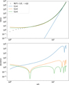 |
Fig. 1 Upper panel: real part of the incomplete gamma function Γ(−1/2, −a/b)i (black points) with fitting with f1(x) (blue line), f2(x) (orange line), and f3(x) (green line). Lower panel: deviations from the incomplete gamma function. |
2.4 Fitting of the analytic model
For high-mass planets, our analytic formula contains the incomplete gamma function. For practical use, we fit the incomplete gamma function by simpler forms. We tested three types of fitting:
 (20)
(20)
We show the fitting of the function in Fig. 1. We find that the simple power law f1(x) is not enough to fit the function. The fitting with power law and exponential function seems to be well fitted, but we find that f2(x) cannot reproduce the equivalent width because of the relatively small deviation at high x values. In the fitting with f3(x), we added the asymptotic function and confirmed that the f3(x) can reproduce the equivalent width with the exact incomplete gamma function. The fitting parameters for f3(x) are γ1 = 0.019607711263469527,γ2 = 0.8094995623133185,γ3 = 0.39743620918312733,γ4 = −0.4886404403069673, and γ5 = 1.0464152457944846.
3 One-dimensional radiation-hydrodynamic simulations with metal cooling
The temperature of the planetary upper atmosphere depends on many stellar and planetary parameters. To test our analytical model, we performed one-dimensional (1D) radiationhydrodynamic simulations. In this section we introduce the metal cooling dependence of the atmospheric temperature and the equivalent width of helium absorption. We used the ATES code (Caldiroli et al. 2021) to calculate the 1D atmospheric profile including a self-consistent helium triplet population. We set the EUV spectra to 100 times that of GJ 876 spectra from the MUSCLE treasury survey (Loyd et al. 2016) and the far ultraviolet (FUV) to the same value. This choice was intended to mimic systems in which the He I 10 830 Å line is most easily detectable, i.e., with strong EUV-driven escape and relatively weak FUV photoionization from the metastable level. At fixed EUV flux, increasing the FUV flux would enhance the photoionization of metastable helium and thus reduce the metastable fraction and the resulting equivalent width at a given mass-loss rate, whereas lowering the EUV flux would generally decrease the mass-loss rate and metastable He density. A comprehensive exploration of the full EUV-FUV parameter space is left for future work. For low-mass host stars with weak FUV flux, the metastable helium fraction is almost independent of FUV flux (Oklopčić 2019). Our model is valid for young close-in planets around low-mass stars with strong EUV and weak FUV flux. We confirmed that the equivalent width of helium absorption is almost the same even if we assume 100 times FUV flux.
3.1 Basic equations
We solved the following hydrodynamic equations using the ATES code:
 (21)
(21)
 (22)
(22)
 (23)
(23)
where ρ, v, p, E, and H are the gas density, velocity, pressure, energy, and enthalpy per unit volume of gas. The effective gravitational potential Ψ can be given by Ψ = − GMp/r - GM*/r* - GM*r*2/2l3 where l, r* represent the semimajor axis and local distance to the host star as in Mitani et al. (2022). We used the EUV photoionization heating rate in Γ and the Lyα cooling and metal cooling in Λ. The code and setup were already tested in Mitani et al. (2025). We set the surface density as n(r = Rp) = 1014cm−3 and the temperature 1000 K at the inner boundary.
3.2 Metal cooling effect
We incorporated the Mg cooling rate into the total cooling rate (Λ) in our simulations. Mg cooling is a dominant cooling source in the upper atmosphere of hot Jupiters (Huang et al. 2023; Fossati et al. 2025):
 (24)
(24)
where fMg is the fraction of MgII, ∆E = 4.4 eV, nl, nu, and ncrit are the lower-level, upper-level, and the critical density, and Aul is the Einstein coefficient. The Mg cooling can be a dominant cooling process in the upper atmosphere (Huang et al. 2023). We note that the cooling rate of Mg I and Mg II is similar and our model with Mg II cooling can be applied for planets with Mg II and without Mg I.
We also investigated oxygen cooling to better understand the atmospheres of relatively cool planets where Mg condenses out of the upper atmosphere. Fine structure transitions can serve as a dominant cooling mechanism in such environments. For oxygen cooling, we considered the energy levels 3P2, 3P1, 3P0, 1D2, and 1S0. Assuming statistical equilibrium, we calculated the level populations using collisional excitation and de-excitation rates caused by hydrogen and electrons, as well as Einstein coefficients (Osterbrock 1989; Hollenbach & McKee 1989).
However, other metal species play an important role in the atmosphere of sub-Neptunes (Zhang et al. 2022; Linssen et al. 2024; Kubyshkina et al. 2024). Interestingly, the cooling rate of iron is comparable to that of magnesium, playing a significant role in metal-rich planetary atmospheres. Our model indicates that efficient metal cooling, such as from Mg and Fe, can reduce atmospheric mass loss by lowering temperatures and influencing escape dynamics.
Our analytic formula of the equivalent width does not contain any assumptions on the metal species and the gas temperature determines the results. The formula can be used to understand the temperature of the observed upper atmosphere. We note that the helium-to-hydrogen number fraction in our simulations is fixed at 0.083. This assumption is reasonable for planets with not extremely metal-rich upper atmospheres (Z < 50 Z3). However, the helium fraction remains one of the most significant sources of uncertainty in our model. In the upper atmosphere, the metal-licity is expected to be lower compared to the lower atmosphere due to the condensation of metal species and our assumption is valid for the majority of planets with hydrogen-dominated atmospheres.
In low-temperature planets, Mg atoms can condense into clouds in the lower atmosphere, reducing the abundance of Mg in the upper atmosphere. The condensation temperature of Mg species is approximately 2000 K, so our model, which includes Mg cooling, is applicable to close-in planets with high surface temperatures. Notably, solar-abundance magnesium has been detected in the upper atmosphere of planets with surface temperatures around 1500 K (e.g., HD 209458 b; Vidal-Madjar et al. 2013).
We assumed that the metal composition is similar to the solar value and ran simulations of a gas giant (Mp = 0.7 MJ, Rp = 1.4 RJ, l = 0.05 au) as the fiducial cases to test the planet like HD 209458b, which has been observed in helium. We present the radial profiles of high-mass planets in Fig. 2. Due to Mg cooling, the temperature of metal-rich atmospheres decreases. The metastable helium density remains similar across different metallicities because lower temperatures lead to a higher fraction of helium in the metastable state. We also present the hydrodynamic profiles of low-mass planets (Mp = 10.2 M⊕, Rp = 0.25 RJ, l = 0.05 au) like HD 73583b, (Zhang et al. 2022) in Fig. 3. We also ran simulations with only oxygen line cooling and found that oxygen cooling is negligible for low-metallicity cases (Z < 50 Z⊙). This result is consistent with the previous simulation with oxygen cooling (Zhang et al. 2022). To test our analytical model, we focused on Mg cooling to understand helium absorption in metal-rich planets.
Previous studies (Zhang et al. 2022, 2023; Orell-Miquel et al. 2024) used a rather simple relationship between the mass-loss rate and the equivalent width to estimate the mass-loss rate:
 (25)
(25)
where cs is the sound speed, e and me are the electron charge and mass, c is the speed of light, λ0 = 10 830 Å, and W is the equivalent width. gl and f represent the degeneracy and oscillator strength. We adopted Σglf = 1.62 as previously used in Zhang et al. (2022). In the derivation of Eq. (25), they assumed optically thin limit and the timescale of the replacement of helium triplet τ = R*/cs. In their estimate, the radial profile of density is neglected. Constructing a model for equivalent width with the 1D radial profile is the main goal of this section.
Note that the previous study suggests the metal line absorption of near-ultraviolet radiation is a dominant heating source in the upper atmosphere of ultra-hot Jupiter (Fossati et al. 2025). In this study, we ignored the heating due to the metal absorption because such a cooling is significant only for planets around A-type stars with extreme intense near-ultraviolet luminosity due to the high surface temperature and negligible for many planets.
 |
Fig. 2 Radial profiles of the temperature (top), metastable helium density (upper middle), heating and cooling rate (lower middle), and neutral fraction (nneutral/ntotal; bottom) with high-mass planets of different metallicities (Mp = 0.7MJ, Rp = 1.4 RJ, l = 0.05 au, FEUV = 5600 erg/s/cm2, and Z = 0,10 Z⊙, 30 Z⊙). The photoionization heating (solid), Mg cooling (dashed), and Lyα cooling (dotted) are shown in the bottom panel. |
3.3 Post-processing other metal cooling effects
In real atmospheres, radiative cooling by multiple metal species can further reduce the temperature, as demonstrated in previous studies (Zhang et al. 2023; Linssen et al. 2024; Kubyshkina et al. 2024; Fossati et al. 2025). To assess this effect, we computed the metal cooling rate in post-processing using the sunbather module (Linssen et al. 2024), which is based on the open-source code CLOUDY (Chatzikos et al. 2023). We used the hydrodynamic profile from our simulations and calculated the heating and cooling rate by sunbather module to check how the detailed metal coolings change the atmospheric temperature structure. We note that our analytical models assume the isothermal profile of atmosphere and isotropic helium metastable state fraction and are independent of the dominant cooling process.
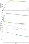 |
Fig. 3 Same as Fig. 2 but for low-mass planets (Mp = 10.2 M⊕, Rp = 0.25 RJ, l = 0.05 au, and FEUV = 5600 erg/s/cm2). |
3.4 Thermospheric balance temperature with metal cooling
If the EUV flux is sufficiently large, the gas temperature reaches high enough level that the radiative cooling dominates the cooling process. We estimated the gas temperature where the radiative cooling balances the photoionization heating at the base as in Mitani et al. (2025):
 (26)
(26)
We assumed a monochromatic EUV (hν1 = 20 eV) to estimate the base density where the outflow launched by EUV photoheating for simplicity. Note that the base density depends on the EUV spectrum within a factor of 2 as in Mitani et al. (2025). Figure 4 shows the metallicity dependence of the gas temperature. Our simple estimate from Eq. (26) represents the metallicity dependence of gas temperature qualitatively well. We find that the metallicity dependence of the temperature can be given by a power law. We fit the metallicity dependence of the thermospheric balance temperature in the range Z⊙ ≤ Z ≤ 100 Z⊙ and get
 (27)
(27)
where T0 = 7562K, β = −0.1146. We note that the gas thermospheric balance temperature is determined by Lyα cooling and becomes ~104 K for planets without metal cooling. We also confirm that the metallicity dependence of the thermospheric balance temperature is similar in weak-gravity planets.
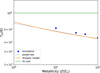 |
Fig. 4 Thermospheric balance gas temperatures as a function of metal-licity. The temperature from Eq. (26) - with the orange and green curves representing Mg and OI cooling - and the gas temperature at the sonic point from simulations (dots) are shown. The power-law fit of Eq. (27) is also shown as a dotted curve. |
4 Comparison of the analytical model and simulations
In this section we compare the analytical model described in Sect. 2 with our simulations described in Sect. 3. We also compare our analytical model with the previous relationship between the mass-loss rate and equivalent width (see Eq. (5)).
4.1 High-mass planets
In the case of atmosphere irradiated by hard EUV such as M stars, the fraction of He triplet was approximated as in Oklopčić (2019):
 (28)
(28)
where Φ1 is the photoionization rate of the helium ground state. In the case of high-mass planets, the sound crossing timescale τadv = Rp/cs is longer than the r photoionization timescale of the helium ground state and the last term in Eq. (28) can be neglected. We performed 1D simulations of hot Jupiters (Mp = 0.7 MJ, Rp = 1010cm) with different metallicity. We also calculated the equivalent width from Eq. (10) with different thermospheric balance temperatures and sound speed  . Figure 5 shows the derived equivalent width with the mass-loss rate Ṁ = πRs2ρscs. We also compare our analytical model to the previous order-of-magnitude estimate in Eq. (25) and the simulation results.
Our simulations and analytical model suggest the existence of a lower limit for the equivalent width. The low temperature leads to a low-density profile and a high fraction of He triplet, as described in Eq. (28). These two effects almost cancel each other out, making the equivalent width almost independent of metallicity (temperature). For hot Jupiters exposed to high EUV flux, order-of-magnitude estimates may overestimate the massloss rate. Estimating the mass-loss rate of hot Jupiters based on helium triplet equivalent width is challenging because the equivalent width depends only weakly on the mass-loss rate.
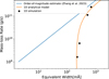 |
Fig. 5 Relationship between the equivalent width and the mass-loss rate. The blue curve represents the order-of-magnitude estimate by Zhang et al. (2023). The orange curve represents our 1D analytical model. The results of our 1D simulations with different metallicity (Z = 0,1,10,30Z⊙) are shown as black dots. |
4.2 Low-mass planets
For low-mass planets with small a, the equivalent width can be given as (see Sect. 2.3)
 (29)
(29)
In low-mass planets with low UV flux, the effect of advection cannot be neglected and the last term in Eq. (28) becomes dominant; we take the effect of advection into account as in Oklopčić (2019). We also calculated the equivalent width for low-mass planets (e.g., HD 73583b: Mp = 10.2 M⊕, Rp = 0.25 RJ, R* = 0.63 R⊙, and FEUV = 5600 erg/s/cm2) with different temperatures (3000 K < T < 15 000K). The ionization fraction of hydrogen is not large at low altitudes, and we can assume the mean molecular weight there is μ ≈ 1. Figure 6 shows our analytical model and the results of different simulations. Our analytical model suggests an equivalent width that is insensitive to the mass-loss rates. We find that the equivalent width from our simulations is larger than that from the previous study because the helium metastable fraction of the previous study is lower than ours. This is because the high temperature in the upper atmosphere of the previous study leads to a high rate of recombination into the triplet state. The density profile difference in our analytical models is within a factor of 2 in the case of a temperature-dependent metastable helium fraction. Our analytical method is valid for general planets. To understand the relationships between the mass-loss rate and the equivalent width, we tested our models with fixed parameters (T = 5000 K, f3 = 10−6) and found that our analytical model reproduces the behavior of the previous study under this assumption (red solid line in Fig. 6). The previous estimate (Eq. (25)) is better suited for low-mass planets than for high-mass planets because the density structure of low-mass planets is not steep and the radial dependence of the optical depth is not significant.
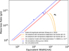 |
Fig. 6 Same as Fig. 5 but for low-mass planets. Solid curves represent our 1D analytical model with a temperature-dependent helium metastable fraction (orange) and with a fixed temperature and helium metastable fraction (red). The results of our 1D simulations (Z = 0,1,10, 30 Z⊙) are shown as black dots, and those from Zhang et al. 2023) as blue dots. |
5 Discussions
5.1 Model predictions and observations
Helium triplet absorption has emerged as a crucial probe of the upper atmospheres of close-in exoplanets. Although several recent observations have reported non-detections of this feature, our results can be used to understand the atmospheric properties of such observed planets. Our radiation-hydrodynamic model, which explicitly includes metal cooling, demonstrates that enhanced metal radiative cooling can lower the atmospheric temperature. This reduction, in turn, increases the fraction of helium in its metastable triplet state, offsetting the expected decrease in mass-loss rate. We analyzed the equivalent width of helium triplet absorption using data from the MOPYS project (Orell-Miquel et al. 2024).
In Fig. 7, we present the distribution of estimated equivalent widths of exoplanets with helium triplet observations for low-mass planets. We assumed a gas temperature of Tgas = 5000 K because the metallicity of the atmosphere is usually unknown and the equivalent width is almost independent of the gas temperature. Planets with detection of helium triplet show larger equivalent widths (>10 mÅ) in Eqs. (10) and (29) than that of planets without detection of helium absorption. Our findings suggest that in cases where the observed upper limit of the equivalent width exceeds our prediction, the actual helium triplet fraction may be lower than estimated by Eq. (28). Such a reduction in the triplet fraction could result from additional processes, such as FUV photoionization of metastable helium or the influence of stellar winds, as discussed in Mitani et al. (2022). In Fig. 7 we also present the distribution for high-mass planets. In the case of high-mass planets, the range of model predictions is narrower than that for low-mass planets. Moreover, for low-mass planets, in contrast to Jupiter-mass planets, our model generally predicts lower equivalent widths. This is consistent with the frequent non-detections of helium absorption in sub-Neptunes, which may be due to either a low level of EUV flux or the cooling effects of metals reducing the atmospheric temperature. We computed the mean square error of the predictions. Specifically, we measured the mean square of the residuals in log space as
 (30)
(30)
where EWobs,i and EWpred,i are the equivalent widths of observations and predictions, and N is the total number of observed planets. The corresponding relative errors of our models, exp(RMSlog), are ~5 and ~7 for low-mass and high-mass planets, respectively. The errors are similar in the two cases.
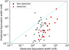
We also tested the prediction from Eq. (25) (see Fig. 8). We calculated the mass-loss rate from the EUV flux from MOPYS, assuming an energy-limited mass-loss rate of
 (31)
(31)
where ε = 0.1 and FEUV are the mass-loss efficiency and EUV flux from the host star. Equation (31) ignores the difference between Rp and the effective radius of EUV absorption (REUV). However, for the low-mass planets in our sample, we typically find REUV ≲ 1.2Rp, so the difference in the resulting mass-loss rates is within a factor of ~ (REUV/Rp)2 ≲ 1.4 (i.e., generally within a factor of ≲2).
The prediction from Eq. (25) tends to underestimate the equivalent width even for planets with detections although the relative error is ~ 6 and close to our models. This trend is inconsistent with the model assumptions that the planets have pure hydrogen-and-helium-dominated atmosphere because metal cooling process and/or stellar wind confinement reduce the mass-loss rate and the equivalent width in real systems. Our model prediction is more consistent not only with the hydrodynamic simulations but also with observations.
The parameter a = GMp/cs2 plays a pivotal role in determining the equivalent width, serving as a key diagnostic of the underlying atmospheric dynamics. Interestingly, our model predicts substantial equivalent width values (exceeding 100 mÅ) for planets such as 55 Cnc e, AU Mic b, and TOI 01235 b, despite the absence of detectable helium absorption. This discrepancy may indicate the presence of nonstandard processes, such as the impact of a strong stellar wind or the possibility of atmospheres that are not hydrogen-dominated. For example, 55 Cnc e is a ultra-short-period exoplanet and hosts a magma ocean. In such systems, the primordial hydrogen atmosphere quickly escapes and a long equivalent width is expected if they have a hydrogen atmosphere. In the case of TOI 1235 b, the planet can also lose the primordial atmosphere (Krishnamurthy et al. 2023). It is difficult to distinguish these planets from the previous simple relationships in Eq. (25) and the energy-limited mass-loss rates but our model prediction is useful to distinguish them from helium observations. In the case of AU Mic b, the stellar wind confinement can modify the outflow structure and reduce the observed signals (McCann et al. 2019; Mitani et al. 2022). Our model is also useful to find the peculiar non-detections from observations.
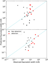 |
Fig. 7 Observed equivalent width and prediction of the equivalent width from our 1D model for low-mass planets (Mp ≤ 0.1 MJ; top) and high-mass planets (Mp > 0.1 MJ; bottom). We use the observational data from the MOPYS project (Orell-Miquel et al. 2024). For planets with non-detections, the triangles show the upper limit of the equivalent width. |
5.2 Other metal cooling effects
We compared our analytical model with the results of hydrodynamic simulations. In these simulations, we included only Mg-ion radiative cooling as the metal cooling mechanism.
In real atmospheres, radiative cooling by multiple metal species can further reduce the temperature, as demonstrated in previous studies (Zhang et al. 2023; Linssen et al. 2024; Kubyshkina et al. 2024; Fossati et al. 2025). To assess this effect, we computed the metal cooling rate in post-processing using the sunbather module (Linssen et al. 2024), which is based on the open-source code CLOUDY (Chatzikos et al. 2023), to check whether the atmospheric temperature is reduced by metal coolings in real systems. We note that our post-processing is not used for the self-consistent calculations but we do not expect the changes in the radiative heating/temperature to affect significantly the mass-loss rate and density.
Figure 9 shows the radial profile of cooling fractions for the Z = 10 Z⊙ case. Near the surface, Mg and Fe ions are the dominant cooling sources, while oxygen ions become dominant in the outer regions. Although the identity of the dominant cooling species varies with metallicity, we find that the overall temperature profile remains nearly independent of which metal ion dominates.
In our post-processing calculations, cooling by metal species other than Mg becomes dominant. Figure 10 shows the atmospheric temperature profiles for different metallicities. Temperatures in metal-rich planets are systematically higher in post-processing because, in addition to EUV hydrogen photoionization heating, we included other photoheating processes; in particular, heating by oxygen ions contributes roughly 10 % of the total heating throughout the atmosphere of these planets. The atmospheric temperature in real systems might be higher (>5000 K) and low mass-loss rate and long equivalent width can be rare. Despite this, the metallicity dependence of the maximum atmospheric temperature closely mirrors that of the Mg-only cooling case, since radiative cooling becomes inefficient at lower temperatures.
We note that our analytical models assume the isothermal profile of the atmosphere and isotropic helium metastable state fraction and are independent of the dominant cooling process.
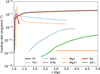 |
Fig. 9 Radial profile of the cooling rate of the Z = 10 Z⊙ case from the post-processing calculation. Only cooling processes with a fraction greater than 0.1 are shown. However, other minor cooling processes not shown in the figure have been included in our calculations. Free-free and free-bound cooling are also shown. |
6 Summary
Helium triplet absorption has been widely used to observe the atmospheric escape of close-in exoplanets. Understanding how helium absorption depends on the temperature of a planetary atmosphere is important for interpreting observations of different metallicities. We derived analytical models for helium absorption that can be used for general close-in planets with a hydrogen-dominated atmosphere. Our analytical models only assume the upper part of the atmosphere to be isothermal, and we assumed an isotropic fraction of metastable helium; the model is generally applicable to close-in planets around low-mass stars with hydrogen-dominated atmospheres. We also performed hydrodynamic simulations and estimate that the equivalent width is weakly dependent on the mass-loss rate in the case of hot Jupiters, which is consistent with the simulations.
We compared our 1D radiation-hydrodynamic model with previous estimates based on the energy-limited mass-loss approach. We find that the latter tends to underestimate the equivalent width. Compared to the estimates in Zhang et al. (2022, 2023), our model provides predictions that are more consistent with the observed values. Our model also predicts longer equivalent widths for ultra-short-period planets. If the planets possessed a primordial hydrogen-dominated atmosphere, the strong outflow launched by intense radiation shows deep absorption. The simple estimation of the mass-loss rate from the equivalent width overestimates the mass-loss rate. This comparison underscores the necessity of incorporating metal cooling and its associated thermo-chemical effects to accurately interpret helium triplet observations. We tested the different metal cooling species and find that the maximum temperature for Mg-only is similar to that for other metal species because the metal radiative cooling becomes inefficient at lower temperatures. Our analytical model only uses an assumption on the temperature of the upper atmosphere and is therefore independent of the specific dominant cooling process. Our model provides an easy way to estimate the helium triplet fraction of the systems and can be used to identify planets with helium observations that cannot be explained by simple hydrogen and helium atmospheres. We also find that it is difficult to use a simple estimate from the energy-limited mass-loss rate to identify such planets. In such systems, nonstandard processes such as stellar wind compression or the absence of a primordial hydrogen-rich atmosphere may be required to understand the thermo-chemical structures.
In short, our study presents a comprehensive framework for understanding the interplay between metal species, atmospheric structure, and atmospheric escape processes for close-in exoplanets. By accounting for the influence of metal cooling, we offer a refined interpretation of helium triplet absorption observations. Future work combining detailed observations with advanced modeling will be essential to further unraveling the complex dynamics governing exoplanetary atmospheres.
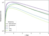 |
Fig. 10 Atmospheric temperature profiles of post-processing calculations with different metallicities: Z = 0,10 Z⊙, and 30 Z⊙. The solid and dashed lines represent the profiles of post-processing calculations and simulations presented in Fig. 2. |
Acknowledgements
We thank the anonymous referee for constructive comments and suggestions, which helped to improve the quality and clarity of this paper. HM has been supported by JSPS Overseas Research Fellowship. This work was supported by JSPS KAKENHI Grant Number 25K17432. Numerical computations were in part carried out on Cray XD2000 at the Center for Computational Astrophysics, National Astronomical Observatory of Japan. RK acknowledges financial support via the Heisenberg Research Grant funded by the Deutsche Forschungsgemeinschaft (DFG, German Research Foundation) under grant no. KU 2849/9, project no. 445783058.
References
- Alam, M. K., Kirk, J., Dos Santos, L. A., et al. 2024, AJ, 168, 102 [Google Scholar]
- Allart, R., Bourrier, V., Lovis, C., et al. 2018, Science, 362, 1384 [Google Scholar]
- Allart, R., Lemée-Joliecoeur, P. B., Jaziri, A. Y., et al. 2023, A&A, 677, A164 [NASA ADS] [CrossRef] [EDP Sciences] [Google Scholar]
- Ballabio, G., & Owen, J. E. 2025, MNRAS, 537, 1305 [Google Scholar]
- Ben-Jaffel, L., Ballester, G. E., García Muñoz, A., et al. 2022, Nat. Astron., 6, 141 [NASA ADS] [CrossRef] [Google Scholar]
- Bennett, K. A., Redfield, S., Oklopčić, A., et al. 2023, AJ, 165, 264 [NASA ADS] [CrossRef] [Google Scholar]
- Boehm, V. A., Lewis, N. K., Fairman, C. E., et al. 2025, AJ, 169, 23 [Google Scholar]
- Bourrier, V., Lecavelier des Etangs, A., Ehrenreich, D., et al. 2018, A&A, 620, A147 [NASA ADS] [CrossRef] [EDP Sciences] [Google Scholar]
- Caldiroli, A., Haardt, F., Gallo, E., et al. 2021, A&A, 655, A30 [NASA ADS] [CrossRef] [EDP Sciences] [Google Scholar]
- Carolan, S., Vidotto, A. A., Plavchan, P., Villarreal D’Angelo, C., & Hazra, G. 2020, MNRAS, 498, L53 [NASA ADS] [CrossRef] [Google Scholar]
- Chatzikos, M., Bianchi, S., Camilloni, F., et al. 2023, Rev. Mexicana Astron. Astrofis., 59, 327 [Google Scholar]
- Ehrenreich, D., Bourrier, V., Wheatley, P. J., et al. 2015, Nature, 522, 459 [Google Scholar]
- Fossati, L., Sreejith, A. G., Koskinen, T., et al. 2025, A&A, 699, A186 [NASA ADS] [CrossRef] [EDP Sciences] [Google Scholar]
- Fulton, B. J., Petigura, E. A., Howard, A. W., et al. 2017, AJ, 154, 109 [Google Scholar]
- García Muñoz, A. 2007, Planet. Space Sci., 55, 1426 [Google Scholar]
- García Muñoz, A. 2023, A&A, 672, A77 [NASA ADS] [CrossRef] [EDP Sciences] [Google Scholar]
- Hollenbach, D., & McKee, C. F. 1989, ApJ, 342, 306 [Google Scholar]
- Huang, C., Koskinen, T., Lavvas, P., & Fossati, L. 2023, ApJ, 951, 123 [NASA ADS] [CrossRef] [Google Scholar]
- Kirk, J., Dos Santos, L. A., López-Morales, M., et al. 2022, AJ, 164, 24 [NASA ADS] [CrossRef] [Google Scholar]
- Koskinen, T. T., Yelle, R. V., Lavvas, P. Y-K., & Cho, J. 2014, ApJ, 796, 16 [NASA ADS] [CrossRef] [Google Scholar]
- Koskinen, T. T., Lavvas, P., Huang, C., et al. 2022, ApJ, 929, 52 [NASA ADS] [CrossRef] [Google Scholar]
- Krishnamurthy, V., Hirano, T., Gaidos, E., et al. 2023, MNRAS, 521, 1210 [NASA ADS] [CrossRef] [Google Scholar]
- Kubyshkina, D., Fossati, L., & Erkaev, N. V. 2024, A&A, 684, A26 [NASA ADS] [CrossRef] [EDP Sciences] [Google Scholar]
- Linssen, D. C., Oklopčić, A., & MacLeod, M. 2022, A&A, 667, A54 [NASA ADS] [CrossRef] [EDP Sciences] [Google Scholar]
- Linssen, D., Shih, J., MacLeod, M., & Oklopčić, A. 2024, A&A, 688, A43 [NASA ADS] [CrossRef] [EDP Sciences] [Google Scholar]
- Loyd, R. O. P., France, K., Youngblood, A., et al. 2016, ApJ, 824, 102 [NASA ADS] [CrossRef] [Google Scholar]
- Mazeh, T., Holczer, T., & Faigler, S. 2016, A&A, 589, A75 [NASA ADS] [CrossRef] [EDP Sciences] [Google Scholar]
- McCann, J., Murray-Clay, R. A., Kratter, K., & Krumholz, M. R. 2019, ApJ, 873, 89 [NASA ADS] [CrossRef] [Google Scholar]
- Mitani, H., Nakatani, R., & Yoshida, N. 2022, MNRAS, 512, 855 [NASA ADS] [CrossRef] [Google Scholar]
- Mitani, H., Nakatani, R., & Kuiper, R. 2025, A&A, 695, A153 [NASA ADS] [CrossRef] [EDP Sciences] [Google Scholar]
- Oklopčić, A. 2019, ApJ, 881, 133 [Google Scholar]
- Oklopčić, A., & Hirata, C. M. 2018, ApJ, 855, L11 [Google Scholar]
- Orell-Miquel, J., Murgas, F., Pallé, E., et al. 2024, A&A, 689, A179 [NASA ADS] [CrossRef] [EDP Sciences] [Google Scholar]
- Osterbrock, D. E. 1989, Astrophysics of Gaseous Nebulae and Active Galactic Nuclei (Mill Valley, CA: University Science Books) [Google Scholar]
- Owen, J. E. 2019, Annual Review of Earth and Planetary Sciences, 47, 67 [Google Scholar]
- Owen, J. E., & Wu, Y. 2017, ApJ, 847, 29 [Google Scholar]
- Owen, J. E., Murray-Clay, R. A., Schreyer, E., et al. 2023, MNRAS, 518, 4357 [Google Scholar]
- Rockcliffe, K. E., Newton, E. R., Youngblood, A., et al. 2021, AJ, 162, 116 [NASA ADS] [CrossRef] [Google Scholar]
- Schreyer, E., Owen, J. E., Loyd, R. O. P., & Murray-Clay, R. 2024, MNRAS, 533, 3296 [Google Scholar]
- Sing, D. K., Lavvas, P., Ballester, G. E., et al. 2019, AJ, 158, 91 [Google Scholar]
- Spake, J. J., Sing, D. K., Evans, T. M., et al. 2018, Nature, 557, 68 [Google Scholar]
- Vidal-Madjar, A., Lecavelier des Etangs, A., Désert, J. M., et al. 2003, Nature, 422, 143 [Google Scholar]
- Vidal-Madjar, A., Huitson, C. M., Bourrier, V., et al. 2013, A&A, 560, A54 [NASA ADS] [CrossRef] [EDP Sciences] [Google Scholar]
- Yoshida, T., & Gaidos, E. 2025, A&A, 696, L13 [NASA ADS] [CrossRef] [EDP Sciences] [Google Scholar]
- Zhang, M., Knutson, H. A., Wang, L., Dai, F., & Barragán, O. 2022, AJ, 163, 67 [NASA ADS] [CrossRef] [Google Scholar]
- Zhang, M., Dai, F., Bean, J. L., Knutson, H. A., & Rescigno, F. 2023, ApJ, 953, L25 [NASA ADS] [CrossRef] [Google Scholar]
Appendix A The metastable helium fraction
Our analytical model assumes a constant metastable helium fraction because we focus on young planetary systems around low-mass stars, where the assumption of a constant f3 with height is valid. Figure A.1 shows the f3 profile from our simulations of low-mass planets. The effect of the altitude dependence of f3 remains within a factor of 2 across almost the entire region of our simulations.
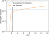 |
Fig. A.1 Helium metastable fraction of low-mass planets with Z = 10Z⊙. The orange line represent the simulation result and the blue line the constant fraction from the thermospheric balance temperature. The dashed line shows the position of the sonic point. |
Appendix B Planetary parameters and model predictions
This appendix summarizes the planetary parameters adopted in the modeling and the predicted equivalent widths shown in Fig. 7. The observational data are taken from the MOPYS compilation (Orell-Miquel et al. 2024), and we computed the equivalent width from the published measurements.
Low-mass planet samples from MOPYS (Orell-Miquel et al. 2024).
All Tables
All Figures
|
Fig. 1 Upper panel: real part of the incomplete gamma function Γ(−1/2, −a/b)i (black points) with fitting with f1(x) (blue line), f2(x) (orange line), and f3(x) (green line). Lower panel: deviations from the incomplete gamma function. |
| In the text | |
|
Fig. 2 Radial profiles of the temperature (top), metastable helium density (upper middle), heating and cooling rate (lower middle), and neutral fraction (nneutral/ntotal; bottom) with high-mass planets of different metallicities (Mp = 0.7MJ, Rp = 1.4 RJ, l = 0.05 au, FEUV = 5600 erg/s/cm2, and Z = 0,10 Z⊙, 30 Z⊙). The photoionization heating (solid), Mg cooling (dashed), and Lyα cooling (dotted) are shown in the bottom panel. |
| In the text | |
|
Fig. 3 Same as Fig. 2 but for low-mass planets (Mp = 10.2 M⊕, Rp = 0.25 RJ, l = 0.05 au, and FEUV = 5600 erg/s/cm2). |
| In the text | |
|
Fig. 4 Thermospheric balance gas temperatures as a function of metal-licity. The temperature from Eq. (26) - with the orange and green curves representing Mg and OI cooling - and the gas temperature at the sonic point from simulations (dots) are shown. The power-law fit of Eq. (27) is also shown as a dotted curve. |
| In the text | |
|
Fig. 5 Relationship between the equivalent width and the mass-loss rate. The blue curve represents the order-of-magnitude estimate by Zhang et al. (2023). The orange curve represents our 1D analytical model. The results of our 1D simulations with different metallicity (Z = 0,1,10,30Z⊙) are shown as black dots. |
| In the text | |
|
Fig. 6 Same as Fig. 5 but for low-mass planets. Solid curves represent our 1D analytical model with a temperature-dependent helium metastable fraction (orange) and with a fixed temperature and helium metastable fraction (red). The results of our 1D simulations (Z = 0,1,10, 30 Z⊙) are shown as black dots, and those from Zhang et al. 2023) as blue dots. |
| In the text | |
|
Fig. 7 Observed equivalent width and prediction of the equivalent width from our 1D model for low-mass planets (Mp ≤ 0.1 MJ; top) and high-mass planets (Mp > 0.1 MJ; bottom). We use the observational data from the MOPYS project (Orell-Miquel et al. 2024). For planets with non-detections, the triangles show the upper limit of the equivalent width. |
| In the text | |
|
Fig. 9 Radial profile of the cooling rate of the Z = 10 Z⊙ case from the post-processing calculation. Only cooling processes with a fraction greater than 0.1 are shown. However, other minor cooling processes not shown in the figure have been included in our calculations. Free-free and free-bound cooling are also shown. |
| In the text | |
|
Fig. 10 Atmospheric temperature profiles of post-processing calculations with different metallicities: Z = 0,10 Z⊙, and 30 Z⊙. The solid and dashed lines represent the profiles of post-processing calculations and simulations presented in Fig. 2. |
| In the text | |
|
Fig. A.1 Helium metastable fraction of low-mass planets with Z = 10Z⊙. The orange line represent the simulation result and the blue line the constant fraction from the thermospheric balance temperature. The dashed line shows the position of the sonic point. |
| In the text | |
Current usage metrics show cumulative count of Article Views (full-text article views including HTML views, PDF and ePub downloads, according to the available data) and Abstracts Views on Vision4Press platform.
Data correspond to usage on the plateform after 2015. The current usage metrics is available 48-96 hours after online publication and is updated daily on week days.
Initial download of the metrics may take a while.