| Issue |
A&A
Volume 707, March 2026
|
|
|---|---|---|
| Article Number | A82 | |
| Number of page(s) | 11 | |
| Section | The Sun and the Heliosphere | |
| DOI | https://doi.org/10.1051/0004-6361/202557162 | |
| Published online | 02 March 2026 | |
Failed ejection and oscillations of a current-carrying filament balanced by gravity
1
University of South Bohemia, Faculty of Science, Department of Physics Branišovská 1760 CZ – 370 05 České Budějovice, Czech Republic
2
Astronomical Institute of the Czech Academy of Sciences Fričova 258 CZ – 251 65 Ondřejov, Czech Republic
★ Corresponding author: This email address is being protected from spambots. You need JavaScript enabled to view it.
Received:
9
September
2025
Accepted:
19
January
2026
Abstract
Context. Solar filaments are often associated with solar eruptions and coronal mass ejections. However, in some cases, the ejection process is halted, resulting in a failed eruption. Understanding the processes that occur after filament destabilization is therefore of great importance.
Aims. In this study, we investigate the post-destabilization evolution of a filament in a gravity-balanced model.
Methods. We adopted the filament model, in which a dense filament is supported against gravity by the repulsive force between the filament current and its sub-photospheric image. We first performed an analytical investigation of this model. For the numerical study, we used a two-dimensional magnetohydrodynamic (MHD) model that solved the MHD equations with the Lare2d numerical code.
Results. In this filament model, analytical expressions were derived for the electric current density, plasma density, and their spatial distributions as functions of the model parameters. The total electric current and the filament weight were also calculated. For the numerical simulations, we constructed an equilibrium filament characterized by a magnetic field of B0 = 10−3 T, a mass density ρ0 ∼ 1.3 × 10⁻⁹ kg m−3, and temperature T ∼ 13 000 K. The system was destabilized either by increasing the currents or by reducing the filament density, and its evolution was computed. In both destabilization regimes, the filament was ejected, then halted at a certain altitude, and subsequently fell back, repeating this cycle with a period of about 600 s. The maximum filament ejection velocity was approximately 80 and 40 km s−1, respectively. Beneath the ejected filament, a current sheet forms, where magnetic reconnection occurs. The maximum ejection altitudes were determined as functions of both the destabilizing currents and the degree of filament plasma dilution. Finally, we compared results of this MHD model with those of an ideal vacuum model and discussed all of the results.
Key words: magnetohydrodynamics (MHD) / methods: numerical / Sun: filaments, prominences / Sun: flares
© The Authors 2026
 Open Access article, published by EDP Sciences, under the terms of the Creative Commons Attribution License (https://creativecommons.org/licenses/by/4.0), which permits unrestricted use, distribution, and reproduction in any medium, provided the original work is properly cited.
This article is published in open access under the Subscribe to Open model. This email address is being protected from spambots. You need JavaScript enabled to view it. to support open access publication.
1. Introduction
Solar filaments, also known as prominences, are dense and cool plasma structures (with a particle concentration of 1010 − 1012 cm−3 and a temperature in the coldest part ranging from 5000 to 20 000 K), suspended in the solar corona (Tandberg-Hanssen 1995; Schwartz et al. 2019; Solov’ev 2024). They are often associated with solar eruptions and coronal mass ejections (CMEs). Several models describe these filaments (see, e.g. Priest 2014). Among them, the inverse-polarity model appears to be the most significant. The first such model, proposed by Kuperus & Raadu (1974), considered a circular filament (prominence) carrying an electric current that forms at a certain height within a vertical current sheet. In this model, the dense filament is supported against gravity by the upward Lorentz (repulsive) force between the filament current and its sub-photospheric image current. This model was later extended by including the effect of an external coronal magnetic field (van Tend & Kuperus 1978). In this extended model, and within the so-called strong magnetic field approximation, Forbes & Isenberg (1991) neglected gravity and investigated the mechanism of filament ejection. Later, a model similar to that of Kuperus & Raadu (1974) was proposed by Solov’ev (2010).
On the other hand, Titov & Démoulin (1999) developed a model in which the repulsive force between the filament current and its mirror current is balanced by a surrounding potential magnetic field. This model has been widely and successfully used in numerical simulations of solar flares and CMEs (see, for example, Török et al. 2024; Liu et al. 2024). However, a key limitation of these simulations is the assumption of a zero plasma beta, which neglects the effects of gravity.
Such simplifications, although computationally efficient, may lead to inaccuracies when modelling the filament stability under realistic coronal conditions, where finite plasma pressure and gravitational stratification play significant roles (Fan 2005; Hillier & van Ballegooijen 2013). Moreover, recent observations suggest that the mass loading and thermal structuring of filaments may crucially affect their evolution and eventual eruption (Gibson 2018). These factors can influence the threshold for instability, as well as the nonlinear dynamics of the eruption process. Filament eruptions are often interpreted in terms of ideal magnetohydrodynamic (MHD) instabilities, such as the torus and kink instabilities, which depend on the geometry of the magnetic field and current distribution (Kliem & Török 2006; Aulanier et al. 2010). The onset of these instabilities may be triggered either by slow quasi-static evolution due to photospheric motions or by impulsive external perturbations. Therefore, developing models that include gravitational forces, finite plasma beta, and realistic current configurations is essential for understanding the pre-eruption equilibrium and the conditions under which filaments lose stability. Observationally, filaments appear as dark, elongated structures in H-alpha or extreme-ultraviolet images when viewed against the solar disk, and as bright prominences above the limb. Their internal structure reveals fine-scale threads aligned with the local magnetic field, indicating a strong coupling between thermodynamic and magnetic properties. However, the precise magnetic topology of filaments remains difficult to determine directly due to limitations in coronal magnetic field measurements (Mackay et al. 2010; Parenti 2014). As a result, theoretical and numerical models remain crucial for interpreting observational data and for exploring the mechanisms of filament formation and destabilization. The long-term stability of filaments also depends on their anchoring in the chromosphere and on the large-scale magnetic environment of the corona. In particular, the overlying magnetic arcade can provide stabilizing tension, and its gradual evolution can lead to a loss in equilibrium. Models that can account for these multi-scale processes, including magnetic reconnection and current dissipation, are necessary to fully capture the physics of filament eruptions.
In this paper, we consider the Solov’ev filament model (Solov’ev 2010), in which the repulsive force between the filament current and its mirror current is balanced by gravity. Our objective is to investigate what occurs after a filament in this gravity-balanced configuration becomes destabilized.
The paper is structured as follows: Section 2 introduces the filament model and its analytical analysis. Section 3 describes the corresponding numerical MHD model. Section 4 presents the results. Finally, Section 5 discusses the results in comparison with those of the ideal vacuum model presented in the Appendix, and Section 6 presents the conclusions.
2. Filament model
We used the two-dimensional (2D) filament model proposed by Solov’ev (2010, 2012). In this model, the filament, carrying an electric current, is in equilibrium due to its own weight within the gravitationally stratified solar atmosphere. The magnetic field components Bx and By in the plane intersecting the filament are expressed via the vector potential A, ensuring that the solenoidal condition, which requires the divergence of the magnetic field to be zero, is automatically satisfied,
 (1)
(1)
as
![Mathematical equation: $$ \begin{aligned} B_x = B_\mathrm{0} \frac{1 + k^2 x^2 - k^2 (y - h_0)^2}{[1 + k^2 x^2 + k^2(y - h_0)^2]^2} \end{aligned} $$](/articles/aa/full_html/2026/03/aa57162-25/aa57162-25-eq2.gif) (2)
(2)
and
![Mathematical equation: $$ \begin{aligned} B_y = B_\mathrm{0} \frac{2 k^2 x (y - h_0)}{[1 + k^2 x^2 + k^2(y - h_0)^2]^2}, \end{aligned} $$](/articles/aa/full_html/2026/03/aa57162-25/aa57162-25-eq3.gif) (3)
(3)
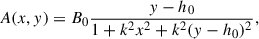
where x and y are the spatial coordinates, k is a free parameter, which defines the scale of the system, and B0 is the magnetic field at h0, which is the height of the centre of the double structure of the filament (the centre between the coronal and sub-photospheric parts). Analysing Eq. (1), the locations of the extremes of the vector potential A(x, y) are in
 (4)
(4)
Similarly, analysing Eq. (2), the locations of the extremes of magnetic field component Bx are at
 (5)
(5)
and the locations of Bx = 0 are at
 (6)
(6)
On the other hand, the magnetic field component Bz, which is perpendicular to the x–y plane, is expressed as (Jelínek et al. 2020)
![Mathematical equation: $$ \begin{aligned} B_z^2(x,y) = B_{ex}^2 -B_0^2\frac{\alpha ^2k^2(y-h_0)^2}{[1+k^2x^2+k^2(y-h_0)^2]^2}, \end{aligned} $$](/articles/aa/full_html/2026/03/aa57162-25/aa57162-25-eq7.gif) (7)
(7)
where α is an arbitrary positive constant and Bex is an external magnetic field at infinity. The parameter α determines the twist of the magnetic field lines in the filament.
Finally, the mass density and pressure distribution in the model are (Jelínek et al. 2020)
![Mathematical equation: $$ \begin{aligned} \varrho (x,y) = \varrho _h(y) +\frac{B_0^2}{2 \mu _0 g_\odot } \frac{8 k^2 (y-h_0)}{[1 + k^2x^2 +k^2(y-h_0)^2]^4} \end{aligned} $$](/articles/aa/full_html/2026/03/aa57162-25/aa57162-25-eq8.gif) (8)
(8)
and
 (9)
(9)
where μ0 = 1.26 × 10⁻⁶ Hm−1 is the vacuum magnetic permeability and g⊙ = 274 ms−2 is the gravitational acceleration at the Sun. Here, 𝜚h(y) is the mass density expressed as (see, e.g. Priest 2014)
 (10)
(10)
and ph(y) is pressure in the gravitationally stratified atmosphere without the filament
 (11)
(11)
where 𝜚0, T0, and p0 are the base mass density, temperature, and pressure (at the photosphere), respectively. The pressure scale height H(y) is determined by the temperature of the plasma and the local gravitational acceleration, and is given by the formula
 (12)
(12)
where  is the mean particle mass and temperature T(y) is defined by Eq. (20).
Using Eqs. (2), (3), and the expression for the electric current density j = (∇×B)/μ0, the z component of this density can be expressed as
![Mathematical equation: $$ \begin{aligned} j_z = \frac{8 B_0}{\mu _0} \frac{k^2(y-h_0)}{[1+k^2x^2+k^2(y-h_0)^2]^3}\cdot \end{aligned} $$](/articles/aa/full_html/2026/03/aa57162-25/aa57162-25-eq14.gif) (13)
(13)
Analysing this relation, the locations of the maximal absolute value of the current density |jz|max are at
 (14)
(14)
For illustration purposes, Figs. 1 and 2 were created using Eq. (13). Figure 1 shows the z component of the electric current density along the y axis (x = 0) for B0 = 10−3 T, h0 = 5 Mm, and three values for parameter k. As shown here, the maximum current density in the region above h0 = 5 Mm increases with the increase in k, but it becomes more localized.
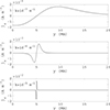 |
Fig. 1. Electric current density (z component) along the y axis (x = 0) for B0 = 10−3 T, h0 = 5 Mm, and three values for parameter k. |
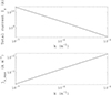 |
Fig. 2. Total electric current (upper panel) in the z direction and the maximum of the z component of the current density (lower panel) in the filament depending on parameter k for B0 = 10−3 T. |
This trend is further confirmed in Figure 2, which shows the dependence of the maximum current density on k. However, as k increases, the total current in the filament, i.e. the current in the entire area above or below h0 = 5 Mm, decreases (Figure 2).
Furthermore, as shown in Figure 3, the filament mass density, expressed only by the second term in Eq. (8) and calculated along the y axis (x = 0), shows a similar profile as for the current density (Figure 1). In this case, the distance between the maximum and minimum of the mass density is  .
.
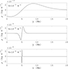 |
Fig. 3. Mass density along the y axis (x = 0) for B0 = 10−3 T, h0 = 5 Mm, and three values for parameter k. |
Finally, Figure 4 shows the weight of the filament per unit length in the direction perpendicular to the x–y plane, as well as the maximum mass density in the filament as a function of parameter k (both calculated from the second term in Eq. (8), i.e. excluding the background atmospheric density). It should be noted that the density at each single grid point – given by the sum of the second term in Eq. (8), which is negative at heights below h0, and the background atmospheric density (the first term in Eq. (8)) – must be positive.
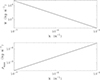 |
Fig. 4. Weight of the filament per one metre in the perpendicular direction to the x–y plane (above h0 = 5 Mm) (upper panel) and the maximum mass density (lower panel) in the filament depending on parameter k for B0 = 10−3 T. |
3. Numerical model
3.1. Governing equations
In the numerical model, we describe plasma dynamics using a set of 2D, time-dependent, resistive, and compressible MHD equations formulated in the Cartesian coordinate system (see, e.g. Goedbloed & Poedts 2004). These equations account for the effects of resistivity and gravity and are expressed using the convective (Lagrangian) derivative
 (15)
(15)
 (16)
(16)
 (17)
(17)
 (18)
(18)
 (19)
(19)
Here, 𝜚 is the mass density, v is the plasma velocity, p is the pressure, ε is the specific internal energy, B is the magnetic field, η is the electrical resistivity, and g represents the gravitational acceleration due to the Sun.
Generally, the terms expressing the radiative losses, Rloss, thermal conduction, Tcond, and heating, H, should be added to the set of MHD equations. Because simulations were performed in an energetically closed model without any external sources, we assume that radiative losses and thermal conduction are fully compensated for by the heating, H; in other words, Rloss + Tcond + H = 0 during the whole studied process.
The simulation domain x ∈ [ − 10, 10] Mm, y ∈ [0, 40] Mm was resolved by a 2000 × 4000 grid, corresponding to the smallest spatial resolution Δx = Δy = 0.01 Mm. This resolution sufficiently covers the studied magnetic structures. User-defined boundary conditions were applied, with the initial values of the variables fixed at the boundaries.
To visualize the simulation data, we used the VisIt software package, which is a free interactive parallel visualization and graphical analysis tool for viewing scientific data (see, e.g., Childs et al. 2012). In addition, MATLAB was used for data processing and supplementary analysis MathWorks (2024).
3.2. The model’s initial equilibrium state
For the filament model, in all of the following simulations, we set the values for the magnetic field B0 and the external magnetic field Bex = 10−3 T, the height of the central double structure h0 = 4.7 Mm, the parameter α = 0.5, and the parameter k = 5 × 10⁻⁷ Mm−1.
As follows from Eqs. (5) and (6), the mass density and pressure consist of two components: (a) the contribution from the solar atmosphere without the filament (ρh(y),ph(y)), and (b) the contribution from the filament itself (the remaining terms in these equations). For the atmospheric component, we first used the temperature profile from the C7 (VAL-C) model of the solar atmosphere (Vernazza et al. 1981; Avrett & Loeser 2008). However, in this case, the magnetic field lines were not sufficiently anchored during the filament ejection.
Therefore, we propose a modified temperature profile that preserves the temperature jump characteristic of the real solar atmosphere (a ratio of about 200), that is, approximately 6000 K in the lower layers (photosphere) and 1.2 MK in the upper layers (corona), but with an abrupt transition in our defined ‘transition region’.
To avoid numerical errors caused by the steep temperature gradient in this area, we expressed the temperature using a hyperbolic tangent function,
![Mathematical equation: $$ \begin{aligned} T(y) = T_{\mathrm{ph} } + \frac{1}{2}(T_{\mathrm{cor} } - T_{\mathrm{ph} }) \cdot \left[1 + \tanh \left(\frac{y - h_{\mathrm{TR} }}{w_\mathrm{TR} } \right) \right], \end{aligned} $$](/articles/aa/full_html/2026/03/aa57162-25/aa57162-25-eq22.gif) (20)
(20)
where Tph = 6000 K is the photospheric temperature, Tcor = 1.2 MK is the coronal temperature, hTR = 5.0 Mm is the height of the transition region as defined in our model, and wTR = 0.01 Mm is the width of this model-defined transition region.
In Figure 5, we present the initial equilibrium state (t = 0 s) for four quantities from our numerical model: the density (blue), temperature (red), absolute value of magnetic field component Bx (green line), and plasma beta parameter β (brown line). The figure also shows two vertical lines indicating the position of the transition region hTR, as defined in our model (solid black line), and the location of the centre of the double structure of the filament h0 (dashed line). The mass density decreases from the lower boundary of the simulation box in agreement with the hydrostatic decrease in the solar gravitational field. At the location of hTR, where the temperature jump occurs, the mass density begins to increase, forming a bump (the modelled filament) with a maximum density of roughly 1.3 × 10⁻⁹ kg m−3. It then decreases again to a value of about 1 × 10⁻¹² kg m−3, which is a typical value in the solar corona. The model temperature follows Eq. (20). Above hTR, in the bump region, which represents the modelled filament, the temperature drops to approximately 13 000 K and then increases to approximately Tcor = 1.2 MK, which is typical of the solar corona.
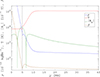 |
Fig. 5. Vertical profiles of the absolute value of the Bx component of the magnetic field (green line), mass density ρ (blue line), temperature T (red line), and plasma beta parameter β (brown line) along the axis of symmetry (x = 0 Mm) in the initial equilibrium state for B0 = 10−3 T and k = 5 × 10⁻⁷ m−1. The vertical, solid black line shows the location of the transition region, hTR = 5 Mm, as defined in our model, while the vertical dotted line denotes the midpoint between the filaments h0 = 4.7 Mm. Note that the y axis is on a logarithmic scale. |
4. Results
In this section, we present the results of numerical simulations aimed at exploring the ejection of the filament owing to its destabilization. Prior to applying any perturbations, we performed a baseline simulation using the equilibrium configuration to verify numerical stability and ensure that the magnetic field and plasma remain stationary in the absence of external changes.
We then considered two destabilizing scenarios: (a) an increase in the electric current in the filament, and (b) a decrease in the filament mass density. In our model, these changes are imposed suddenly for simplicity. In reality, solar processes are more gradual. However, if the current increase or density reduction occurs gradually while the entire filament system is confined by an overlying magnetic field that then suddenly opens, the resulting ejections could resemble the following simulations.
4.1. Failed ejection and oscillations of the filament induced by increasing the electric current
In this case, we started with the model in equilibrium as described above. We then increased both the upper and lower electric currents and analysed the resulting dynamical evolution of the system.
The increased current in the model was achieved by increasing B compared to its initial value B0. Other parameters were not changed. As an example, here we present the case where the magnetic field strength B0 is increased by a factor of 4.
The results of the simulations are presented in Figure 6. The figure shows the temporal evolution of the mass density (brown colour scale) and the magnetic field, which is represented by using the magnetic vector potential and is illustrated in the figure with solid grey lines.
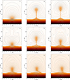 |
Fig. 6. Time evolution of the mass density and magnetic field lines, using the vector potential, represented by solid grey lines, for nine different times t = 0, 168, 280, 628, 897, 1121, 2240, 2800, and 3360 s (a–i, respectively) – the case with the increased electric current. The associated movie is available online. |
The first panel (a) shows the distribution of these quantities in the initial state. The destabilization of the system leads to the ejection of the filament upwards, caused by the increased magnetic force acting between the upper and lower currents. The lower currents remain stationary as they are sufficiently anchored in the dense layers of the atmosphere. Panel (b) shows the situation at time t = 168 s, when the filament is ejected and rises upwards. Panel (c) corresponds to the state when the filament has already reached its maximum height, at time t = 280 s.
Then, the filament starts to move downwards towards the dense layers of the solar atmosphere. This is illustrated in panel (d), corresponding to time t = 628 s, when the filament approaches the moment of reaching these dense atmospheric layers. Then it remains nearly stationary for a short time before starting to move upwards again. This is seen in panel (e) at t = 897 s, when the filament reaches a new maximum height, about 3 Mm lower than during the initial ejection. Panel (f) at t = 1121 s shows the filament again descending towards dense atmospheric layers. In the following times, this cycle is repeated with the period of about 600 s. However, as seen in panel (g) at t = 2240 s, the density structure beneath the filament changed from the density distribution symmetric along the vertical axis (x = 0) to that with some asymmetry. This asymmetry in subsequent times leads to displacement of the filament off the vertical axis (x = 0) (panels (h) and (i) at t = 2800 s and t = 3360 s). The evolution of the filament ejection and its descent is shown in the movie, provided in the paper. To verify that the size of the numerical domain does not influence the magnetic field configuration or the maximum height reached by the filament, we performed an additional comparative simulation. The numerical box was extended by a factor of two in the vertical (y) direction, while all other parameters were kept unchanged. The maximum filament height was then compared with what was obtained in the reference case shown in Figure 6. No significant difference was found, confirming that the original vertical extent of the numerical domain is sufficient and does not affect the results.
Below the ejected filament, a current sheet formed. To examine this process in more detail, Figure 7 shows plasma flows (vectors) around the current sheet, represented by the current density jz, at two times: t = 168 s (left) and t = 280 s (right) for the case with 4 B0. These can be compared with panels (b) and (c) of Figure 6. The panels in Figure 7 illustrate how the plasma from both sides of the current sheet is drawn into its region and directed upwards. The structured current sheet (with magnetic islands) and the associated plasma velocity pattern, most evident in the right panel, indicate magnetic reconnection. This reconnection disrupts the magnetic field lines connecting upper and lower currents.
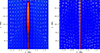 |
Fig. 7. Plasma flows (white arrows) around the current sheet, which are expressed here through the current density jz at two times t = 168 s (left) and 280 s (right) in the case with 4 B0. These panels present details at the same times as panels (b) and (c) in Figure 6. |
The process of filament ejection and its oscillation is also illustrated in Figure 8, which shows the temporal evolution of the distance D between the centre of the upper and lower magnetic structures (with Bx = By = 0). In this figure, two curves are shown, with the blue curve corresponding to the case of an increased electric current. The period of this oscillation is approximately 600 s. The corresponding velocity of the filament ejection and the following oscillations in both cases are shown in Figure 9. As shown here, the maximum velocity of filament ejection was 80 km s−1 in the current-increase case.
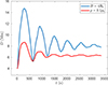 |
Fig. 8. Time evolution of the distance D between the upper and lower magnetic-structure centres (with Bx = By = 0) for two cases with 4 B0 (blue line) and 0.1 ρ0 (red line). |
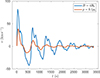 |
Fig. 9. Temporal evolution of the filament ejection velocity v during its ejection and subsequent oscillations for the case with 4 B0 (blue) and the case with 0.1 ρ0 (red). |
In Figure 10, the blue points fitted by the exponential function again correspond to the case of an increased electric current. In this figure, we can see the dependence of the maximum distance Dmax reached between the centres of the upper and lower magnetic structures (with Bx = By = 0). The cases correspond to multiples of the magnetic field 2 B0, 4 B0, 6 B0, 8 B0, and 10 B0 (where B0 = 10−3 T).
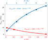 |
Fig. 10. Maximum distance Dmax between the upper and lower magnetic-structure centres (with Bx = By = 0) as a function of multiplication of the initial magnetic field (2 B0, 4 B0, 6 B0, 8 B0, and 10 B0, with B0 = 10−3 T; top x axis) and as a function of the filament density dilution (0.01 ρ0, 0.1 ρ0, and 0.5 ρ0, where ρ0 is the initial density in the filament; bottom x axis). |
4.2. Failed ejection and oscillations of the filament induced by decreasing the mass density
In the second scenario, we again started from the equilibrium model but artificially reduced the mass density of the filament and numerically tracked its subsequent evolution.
In a real filament, such a density decrease may result from plasma heating in a localized region. Heating increases the pressure and decreases the density, which reduces the local weight of the filament and disrupts its equilibrium. The affected segment then begins to rise, while plasma drains from it under the influence of gravity. This further decreases the density in the region and enhances the upward motion.
In Figure 11, we again show the temporal evolution of the density and magnetic field at nine different times, similar to the first studied case described above. Calculations were performed for three different values of the reduced mass density in the filament, namely 0.01 ρ0, 0.1 ρ0, and 0.5 ρ0. The results presented here correspond to the case with ρ = 0.1 ρ0.
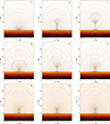 |
Fig. 11. Time evolution of the mass density and magnetic field lines, using the vector potential, represented by solid black lines, for nine different times t = 0, 123, 280, 628, 897, 1121, 2240, 2800, and 3360 s (a–i, respectively) – the case with the evacuation of the filament to 10% of the initial value of the mass density. The associated movie is available online. |
In panel (a), corresponding to time t = 0 s, we again see the initial state. In the following panel (b), at t = 123 s, the filament begins to rise until it reaches the time t = 280 s, as shown in panel (c). Afterwards, the upper filament starts to move downwards towards the lower layers of the atmosphere, which it reaches at approximately t = 628 s, as shown in panel (d). Then it attains another maximum distance between the centres of the two magnetic structures at t = 897 s, as illustrated in panel (e). Panel (f) at t = 1121 s shows the state when the filament again approaches the lower atmospheric layers. This oscillation process is repeated with a period of about 600 s. In the following times, contrary to the case of 4 B0, the filament oscillates up to a stable state along the vertical axis (x = 0) (panels (g), (h), and (i) in t = 2240 s, t = 2800 s, and t = 3360 s. The evolution of filament ejection and its subsequent oscillation are illustrated in the movie included in the paper. As in the previous case, we also performed a comparative simulation to assess the influence of the numerical domain size on the magnetic field configuration and the filament dynamics. No differences in the filament evolution or in the maximum height reached were detected. This is consistent with the fact that, in this density-reduction scenario, the filament reaches a lower height than in the current-increase case, further confirming that the original size of the numerical domain is sufficient and does not affect the results.
In Figure 8, the red curve corresponds to the case with a reduced filament density. The first feature we can observe, when compared with the case of an increased electric current, is that the filament does not reach such a great height as in the current-increase scenario. The second difference is that, in the case of reduced density, the filament reaches its maximum height earlier and remains in this position for a longer duration, approximately 200 s. In contrast, in the case of an increased electric current, the filament reaches its maximum height later and remains close to this maximum for only about half as long, roughly 100 s. However, the figure also shows that despite these differences, the oscillation period of the filament is approximately the same in both cases. The velocity of filament ejection and the following oscillations in this case are shown in Figure 9 by the red line. In this density-reduction case, the maximum velocity of filament ejection is 40 km s−1.
Similarly to the previous case, in Figure 10 we plotted the maximum distance Dmax reached between the centres of the two magnetic structures (red points fitted by the exponential function), but this time for three different values for the reduced initial filament density. The three values considered are 0.01 ρ0, 0.1 ρ0, and 0.5 ρ0. From the plotted values, it is evident that a smaller ratio ρ/ρ0 results in the filament reaching a greater height.
5. Discussion
To understand the origin of the failed ejection and oscillations found, we consider a simple analytical model consisting of two parallel, oppositely directed currents interacting in a vacuum. In equilibrium, the repulsive magnetic force between the currents is balanced by the weight of the upper current (the filament). The lower current is fixed in position. The system is destabilized either by increasing the currents or by reducing the mass of the filament. A detailed description of this model is provided in the Appendix.
As shown in the Appendix, the oscillations arise from the interplay between two forces: the Lorentz force and the filament’s weight. A rough comparison between the oscillations of the distance D obtained from the MHD simulations and the oscillations of height h of the upper current in the ideal vacuum model shows that both the amplitudes and the periods differ significantly (see Figures A.1, A.2, and 8).
Therefore, let us compare the evolution of the height of the upper current above its initial position in the ideal vacuum model with the height of the filament’s maximum current density above its initial position in the MHD model at the very beginning of the ejection. The comparison presented in Figure 12a shows that the evolution of the height in both models destabilized by a current increase is similar up to about 65 s. After this time, however, the evolutions begin to diverge: the height in the MHD model is progressively smaller than in the ideal vacuum model. A similar trend is seen in Figure 12b, where the heights in both models are compared for the case with a reduced filament density. In this case, the divergence appears to begin around 50 s.
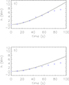 |
Fig. 12. Time evolution of height h of the upper current in the ideal vacuum model (solid lines) and of the filament’s maximum current density in the MHD model (crosses), both measured relative to their initial equilibrium positions, over the 0 − 100 s interval, for the two cases with 4 B0 (panel a) and 0.1 ρ0 (panel b). |
This raises the question of what causes these differences in evolution. The answer lies in plasma processes that are absent in the vacuum model, as well as in the different spatial distributions of currents. In the ideal vacuum model, the currents are localized at specific points, whereas in the MHD model, they are concentrated in some regions. Note also that, in the MHD model, a large region surrounding the maximum current density moves during oscillations as a coherent structure.
In the MHD model, magnetic reconnection is forced by the interaction between the upper and lower currents. This reconnection disrupts some of the magnetic field lines that link the filament current with its sub-photospheric counterpart, thereby reducing the repulsive force between them. Magnetic reconnection begins at the onset of the ejection, after which a current sheet forms beneath the filament. At this stage, reconnection appears to become more effective, as indicated by the divergence of the filament’s current trajectories in the MHD and ideal vacuum models.
Additionally, in the case where destabilization is caused by a reduction in filament mass, the plasma beta parameter is close to unity (0.33 at a height of 6 Mm; see Figure 5). Under such conditions, motions driven by the Lorentz force are suppressed (Priest & Forbes 2000). Moreover, comparing the 0.1 ρ0 and 4 B0 cases, parameter χ is less than ξ2. These facts may explain why the divergence of the filament’s current trajectories begins earlier and why the maximum height reached by the filament is smaller than in the case of destabilization due to an increased current. It should be noted that in the case destabilized by a fourfold increase in a current, the plasma beta parameter is 16 times lower than in the mass-reduction case; consequently, this effect is much less significant.
Comparing the time evolution of the filament in the 4 B0 and 0.1 ρ0 cases in Figures 6 and 11, we see that the evolution in the 4 B0 case is more dynamic. In the 0.1 ρ0 case, the filament settles into a stable state after its damped oscillations, whereas in the 4 B0 case the filament evolves into a state that is displaced from the vertical axis (x = 0). This appears to be caused by some instability in the whole system in the 4 B0 case.
Maximum velocities in the ideal-vacuum model and the MHD models also differ significantly (Figure 9). The velocity profiles vary as well. In the ideal-vacuum model, the velocity profile is smooth and exhibits a single maximum per period, whereas in the MHD model several secondary maxima appear during the filament’s descent. We suggest that these velocity variations arise because some regions beneath the filament become compressed as it falls.
6. Conclusions
For this work, we first studied the Solov’ev model (Solov’ev 2010; Solov’ev 2012) analytically. We derived relations for the electric current density and plasma density and showed their spatial distributions as functions of the model parameters.
Then we investigated the stability and ejection of a gravity-balanced, current-carrying filament using 2D MHD simulations with the Lare2D code. The initial configuration was based on the Solov’ev model, which provides a useful framework for analysing the interplay between magnetic and gravitational forces in filament equilibrium. To study processes after filament destabilization, we considered two types of perturbation. In the first case, the electric currents in the filament system were increased, enhancing the repulsive Lorentz force and driving the filament upwards from its initial equilibrium. In the second case, the plasma density within the filament was reduced relative to its equilibrium value, thereby weakening the stabilizing influence of gravity and allowing the filament to rise
In both cases of destabilization, the filament was ejected upwards. After reaching a certain altitude, it stopped and then began to move downwards, followed by a return upwards, thus performing damped oscillations with a period of about 600 s. The maximum velocity of the filament in the first ejection phase reached about 80 km s−1 in the current-increase case and about 40 km s−1 in the density-reduction case. The maximum altitude attained by the filament during ejection increases with either a higher electric current or lower filament density. These dependencies can be described by exponential functions.
As seen in Figure 8, the filament during oscillations converges to a position that is at a greater height than its initial location. This is because the magnetic reconnection accumulates plasma beneath the filament, thereby supporting it against gravity at a higher altitude.
We found that the current sheet beneath the filament became more pronounced when the filament’s magnetic field lines were more effectively anchored in the dense atmospheric layer below, that is, when the filament structure was embedded deeper in this dense region. Specifically, when the filament structure is embedded more deeply, the magnetic field lines on opposite sides of the current sheet are more antiparallel.
In our MHD model, the current increase or density reduction that destabilizes the filament is suddenly introduced for the sake of simplicity. In reality, solar processes can be more gradual. However, if the current increase or density reduction occurs gradually while the entire filament system is confined by an overlying magnetic field, which then suddenly opens, the resulting ejections could resemble those obtained in our simulations.
Failed eruptions (Gilbert et al. 2007; Mrozek et al. 2024), which begin as typical eruptions but halt in the corona after their initial acceleration for various reasons, may be explained by the simulations presented in this study. The modelled behaviour (an initial rise followed by deceleration and subsequent fallback and oscillations) closely resembles the observed dynamics of such failed eruptions. For example, Kumar et al. (2022) report vertical oscillations of a magnetic flux rope that appear to be similar to those obtained in our simulations, suggesting that the mechanisms described here may have direct observational counterparts.
In summary, our results demonstrate that both current enhancement and density reduction represent viable pathways leading to a failed filament ejection followed by damped oscillatory motion. The simulations reveal that magnetic reconnection beneath the filament and plasma accumulation play key roles in halting the ejection and stabilizing the system. By linking these processes to different modes of destabilization, our study provides new insight into how variations in current and plasma density can give rise to the observed diversity of filament eruption behaviours.
Overall, these findings contribute to a more comprehensive understanding of solar filament dynamics, particularly the transition between successful and failed eruptions. They also highlight the importance of coupling between magnetic and plasma processes in shaping the evolution of solar eruptive events.
Data availability
Movies associated with Figs. 6 and 11 are available at https://www.aanda.org
Acknowledgments
The work in this article is part of the project DynaSun, that has received funding under the Horizon Europe programme of the European Union under grant agreement (no. 101131534). Views and opinions expressed are, however those of the author(s) only and do not necessarily reflect those of the European Union and therefore, the European Union cannot be held responsible for them. MK acknowledges institutional support from the project RVO-67985815. This work was supported by the Ministry of Education, Youth and Sports of the Czech Republic through the e-INFRA CZ (ID:90254).
References
- Aulanier, G., Török, T., Démoulin, P., & DeLuca, E. E. 2010, ApJ, 708, 314 [Google Scholar]
- Avrett, E. H., & Loeser, R. 2008, ApJS, 175, 229 [Google Scholar]
- Childs, H., Brugger, E., Whitlock, B., et al. 2012, in High Performance Visualization-Enabling Extreme-Scale Scientific Insight, 357 [Google Scholar]
- Fan, Y. 2005, ApJ, 630, 543 [NASA ADS] [CrossRef] [Google Scholar]
- Forbes, T. G., & Isenberg, P. A. 1991, ApJ, 373, 294 [Google Scholar]
- Gibson, S. E. 2018, Liv. Rev. Sol. Phys., 15, 7 [Google Scholar]
- Gilbert, H. R., Alexander, D., & Liu, R. 2007, Sol. Phys., 245, 287 [NASA ADS] [CrossRef] [Google Scholar]
- Goedbloed, J. P. H., & Poedts, S. 2004, Principles of Magnetohydrodynamics (Cambridge University Press) [Google Scholar]
- Hillier, A., & van Ballegooijen, A. 2013, ApJ, 766, 126 [Google Scholar]
- Jelínek, P., Karlický, M., Smirnova, V. V., & Solov’ev, A. A. 2020, A&A, 637, A42 [NASA ADS] [CrossRef] [EDP Sciences] [Google Scholar]
- Kliem, B., & Török, T. 2006, Phys. Rev. Lett., 96, 255002 [Google Scholar]
- Kumar, P., Nakariakov, V. M., Karpen, J. T., Richard DeVore, C., & Cho, K.-S. 2022, ApJ, 932, L9 [CrossRef] [Google Scholar]
- Kuperus, M., & Raadu, M. A. 1974, A&A, 31, 189 [NASA ADS] [Google Scholar]
- Liu, Q., Jiang, C., Bian, X., et al. 2024, MNRAS, 529, 761 [Google Scholar]
- Mackay, D. H., Karpen, J. T., Ballester, J. L., Schmieder, B., & Aulanier, G. 2010, Space Sci. Rev., 151, 333 [Google Scholar]
- MathWorks. 2024, MATLAB https://www.mathworks.com/products/matlab.html, version R2024b [Google Scholar]
- Mrozek, T., Li, Z., Karlický, M., et al. 2024, Sol. Phys., 299, 81 [Google Scholar]
- Parenti, S. 2014, Liv. Rev. Sol. Phys., 11, 1 [Google Scholar]
- Priest, E. 2014, Magnetohydrodynamics of the Sun (New York, USA: Cambridge Uni. Press), 391 [Google Scholar]
- Priest, E., & Forbes, T. 2000, Magnetic Reconnection: MHD Theory and Applications (Cambridge University Press) [Google Scholar]
- Schwartz, P., Gunár, S., Jenkins, J. M., et al. 2019, A&A, 631, A146 [NASA ADS] [CrossRef] [EDP Sciences] [Google Scholar]
- Solov’ev, A. A. 2010, Astron. Rep., 54, 86 [Google Scholar]
- Solov’ev, A. A. 2012, Geomagn. Aeron., 52, 1062 [Google Scholar]
- Solov’ev, A. A. 2024, Astrophys. Bull., 79, 508 [Google Scholar]
- Tandberg-Hanssen, E. 1995, The Nature of Solar Prominences (Kluwer Academic Publishers), 199 [Google Scholar]
- Titov, V. S., & Démoulin, P. 1999, A&A, 351, 707 [NASA ADS] [Google Scholar]
- Török, T., Linton, M. G., Leake, J. E., et al. 2024, ApJ, 962, 149 [CrossRef] [Google Scholar]
- van Tend, W., & Kuperus, M. 1978, Sol. Phys., 59, 115 [Google Scholar]
- Vernazza, J. E., Avrett, E. H., & Loeser, R. 1981, ApJS, 45, 635 [Google Scholar]
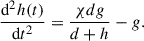
Appendix A: Ideal vacuum model
Let us consider the ideal case of two parallel currents I, oriented in the opposite direction and separated by a distance d in vacuum. The lower current is fixed in position, while the upper current (a filament) has a mass per unit length m. In equilibrium, the repulsive magnetic force between the currents balances the weight of the upper filament (mg), i.e.
 (A.1)
(A.1)
where A =  .
.
Now, let us increase both currents by a factor of ξ. The weight of the upper filament remains the same. The net force acting on the filament can then be written as
 (A.2)
(A.2)
where h denotes the vertical displacement (height) of the upper filament from its equilibrium position.
Hence, the equation of motion for the upper filament becomes
 (A.3)
(A.3)
Substituting  simplifies the equation to
 (A.4)
(A.4)
The right-hand side of this equation depends only on h. Multiplying both sides by by  and integrating yields
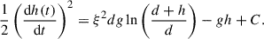 (A.5)
(A.5)
Applying the initial conditions h(t = 0) = 0 and 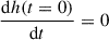 gives C = 0, and thus the first integral is
 (A.6)
(A.6)
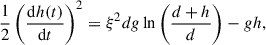
Therefore,
![Mathematical equation: $$ \begin{aligned} \frac{\mathrm{d} h(t)}{\mathrm{d} t} = \sqrt{2 \left[\xi ^2 d g \ln \left(\frac{d+h}{d}\right) - g h\right]}, \end{aligned} $$](/articles/aa/full_html/2026/03/aa57162-25/aa57162-25-eq33.gif) (A.7)
(A.7)
and the implicit time–height relation can be written as
![Mathematical equation: $$ \begin{aligned} t(h) = \int _{0}^{h} \frac{\mathrm{d} h^{\prime }}{\sqrt{2 \left[\xi ^2 d g \ln \left(\frac{d+h}{d}\right) - g h\right]}}, \end{aligned} $$](/articles/aa/full_html/2026/03/aa57162-25/aa57162-25-eq34.gif) (A.8)
(A.8)
This integral has no closed-form elementary solution; therefore, we solved it numerically and inverted it to obtain h(t).
Now, let us consider the case where the filament density is reduced. The force acting on the upper current can then be expressed as
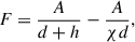 (A.9)
(A.9)
where χ denotes the factor by which the filament density is diluted. The corresponding mass is  . After substituting this into the equation of motion, we obtain
 (A.10)
As can be seen, this equation has the same form as in the case of increased current (Eq. A.4), and thus it can be solved in the same manner.
Note that in the both cases the filament trajectory does not depend on the electric current I and mass m. As an example of the calculations, in Figure A.1 we show the time evolution of the height h and velocity v of the filament for the parameter ξ = 4, which corresponds to the 4 B0 MHD case. Similarly, in Figure A.2 we present the same for the parameter χ = 10, which corresponds to the 0.1 ρ0 MHD case. The both these figures show oscillations.
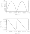 |
Fig. A.1. Time evolution of the height h of the upper current above its initial equilibrium position, and of its velocity v, for the parameter ξ = 4 and d = 1.79 Mm, which corresponds to the 4 B0 MHD case. |
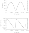 |
Fig. A.2. Time evolution of the height h of the upper current above its initial equilibrium position, and of its velocity v, for the parameter χ = 10 and d = 1.79 Mm, which corresponds to the 0.1 ρ0 MHD case. |
All Figures
|
Fig. 1. Electric current density (z component) along the y axis (x = 0) for B0 = 10−3 T, h0 = 5 Mm, and three values for parameter k. |
| In the text | |
|
Fig. 2. Total electric current (upper panel) in the z direction and the maximum of the z component of the current density (lower panel) in the filament depending on parameter k for B0 = 10−3 T. |
| In the text | |
|
Fig. 3. Mass density along the y axis (x = 0) for B0 = 10−3 T, h0 = 5 Mm, and three values for parameter k. |
| In the text | |
|
Fig. 4. Weight of the filament per one metre in the perpendicular direction to the x–y plane (above h0 = 5 Mm) (upper panel) and the maximum mass density (lower panel) in the filament depending on parameter k for B0 = 10−3 T. |
| In the text | |
|
Fig. 5. Vertical profiles of the absolute value of the Bx component of the magnetic field (green line), mass density ρ (blue line), temperature T (red line), and plasma beta parameter β (brown line) along the axis of symmetry (x = 0 Mm) in the initial equilibrium state for B0 = 10−3 T and k = 5 × 10⁻⁷ m−1. The vertical, solid black line shows the location of the transition region, hTR = 5 Mm, as defined in our model, while the vertical dotted line denotes the midpoint between the filaments h0 = 4.7 Mm. Note that the y axis is on a logarithmic scale. |
| In the text | |
|
Fig. 6. Time evolution of the mass density and magnetic field lines, using the vector potential, represented by solid grey lines, for nine different times t = 0, 168, 280, 628, 897, 1121, 2240, 2800, and 3360 s (a–i, respectively) – the case with the increased electric current. The associated movie is available online. |
| In the text | |
|
Fig. 7. Plasma flows (white arrows) around the current sheet, which are expressed here through the current density jz at two times t = 168 s (left) and 280 s (right) in the case with 4 B0. These panels present details at the same times as panels (b) and (c) in Figure 6. |
| In the text | |
|
Fig. 8. Time evolution of the distance D between the upper and lower magnetic-structure centres (with Bx = By = 0) for two cases with 4 B0 (blue line) and 0.1 ρ0 (red line). |
| In the text | |
|
Fig. 9. Temporal evolution of the filament ejection velocity v during its ejection and subsequent oscillations for the case with 4 B0 (blue) and the case with 0.1 ρ0 (red). |
| In the text | |
|
Fig. 10. Maximum distance Dmax between the upper and lower magnetic-structure centres (with Bx = By = 0) as a function of multiplication of the initial magnetic field (2 B0, 4 B0, 6 B0, 8 B0, and 10 B0, with B0 = 10−3 T; top x axis) and as a function of the filament density dilution (0.01 ρ0, 0.1 ρ0, and 0.5 ρ0, where ρ0 is the initial density in the filament; bottom x axis). |
| In the text | |
|
Fig. 11. Time evolution of the mass density and magnetic field lines, using the vector potential, represented by solid black lines, for nine different times t = 0, 123, 280, 628, 897, 1121, 2240, 2800, and 3360 s (a–i, respectively) – the case with the evacuation of the filament to 10% of the initial value of the mass density. The associated movie is available online. |
| In the text | |
|
Fig. 12. Time evolution of height h of the upper current in the ideal vacuum model (solid lines) and of the filament’s maximum current density in the MHD model (crosses), both measured relative to their initial equilibrium positions, over the 0 − 100 s interval, for the two cases with 4 B0 (panel a) and 0.1 ρ0 (panel b). |
| In the text | |
|
Fig. A.1. Time evolution of the height h of the upper current above its initial equilibrium position, and of its velocity v, for the parameter ξ = 4 and d = 1.79 Mm, which corresponds to the 4 B0 MHD case. |
| In the text | |
|
Fig. A.2. Time evolution of the height h of the upper current above its initial equilibrium position, and of its velocity v, for the parameter χ = 10 and d = 1.79 Mm, which corresponds to the 0.1 ρ0 MHD case. |
| In the text | |
Current usage metrics show cumulative count of Article Views (full-text article views including HTML views, PDF and ePub downloads, according to the available data) and Abstracts Views on Vision4Press platform.
Data correspond to usage on the plateform after 2015. The current usage metrics is available 48-96 hours after online publication and is updated daily on week days.
Initial download of the metrics may take a while.