| Issue |
A&A
Volume 707, March 2026
|
|
|---|---|---|
| Article Number | A129 | |
| Number of page(s) | 17 | |
| Section | Extragalactic astronomy | |
| DOI | https://doi.org/10.1051/0004-6361/202557790 | |
| Published online | 02 March 2026 | |
The slope and scatter of the star-forming main sequence at z ∼ 5: Reconciling observations with simulations
1
Institute of Science and Technology Austria (ISTA) Am Campus 1 3400 Klosterneuburg, Austria
2
MIT Kavli Institute for Astrophysics and Space Research, Massachusetts Institute of Technology Cambridge MA 02139, USA
3
Universite Claude Bernard Lyon 1, CRAL UMR5574, ENS de Lyon, CNRS Villeurbanne F-69622, France
4
Institute for Computational & Data Sciences, The Pennsylvania State University University Park PA 16802, USA
5
Institute for Gravitation and the Cosmos, The Pennsylvania State University University Park PA 16802, USA
6
Department of Astronomy, Oskar Klein Centre, Stockholm University, AlbaNova University Center SE-106 91 Stockholm, Sweden
7
Physics Department, Ben-Gurion University of the Negev PO Box 653 Beer-Sheva 8410501, Israel
8
Niels Bohr Institute, University of Copenhagen Jagtvej 128 2200 Copenhagen N, Denmark
9
Department of Astronomy, University of Geneva Chemin Pegasi 51 1290 Versoix, Switzerland
10
Laboratory of Astrophysics, École Polytechnique Fédérale de Lausanne (EPFL), Observatoire de Sauverny 1290 Versoix, Switzerland
11
Cosmic Dawn Center (DAWN) Copenhagen, Denmark
12
Max-Planck-Institut für Radioastronomie Auf dem Hügel 69 53121 Bonn, Germany
13
INAF – Osservatorio Astronomico di PAdova Vicolo dell’Osservatorio 5 I-35122 Padova, Italy
14
Centro de Astrobiología (CAB), CSIC-INTA, Carretera de Ajalvir km 4 Torrejón de Ardoz E-28850 Madrid, Spain
15
Kavli Institute for Cosmology, University of Cambridge Madingley Road Cambridge CB3 0HA, UK
16
Cavendish Laboratory, University of Cambridge JJ Thomson Avenue Cambridge CB3 0HE, UK
★ Corresponding author: This email address is being protected from spambots. You need JavaScript enabled to view it.
Received:
21
October
2025
Accepted:
6
January
2026
Abstract
Galaxies exhibit a tight correlation between their star formation rate (SFR) and stellar mass over a wide redshift range known as the star-forming main sequence (SFMS). With JWST, the SFMS can now be investigated at high redshifts down to masses of ∼106 M⊙, using sensitive star formation rate tracers such as the Hα emission, which allow us to probe the variability in the star formation histories. We present inferences of the SFMS based on 316 Hα-selected galaxies at z ∼ 4 − 5 with log(M★/M⊙) = 6.4 − 10.6. These galaxies were identified behind the Abell 2744 lensing cluster with NIRCam grism spectroscopy from the survey All the Little Things (ALT). At face value, our data suggest a shallow slope in the SFMS (SFR ∝ M★α, with α = 0.45). After we corrected this for the Hα-flux limited nature of our survey using a Bayesian framework, the slope steepened to α = 0.59+0.10−0.09, whereas current data on their own are inconclusive on the mass dependence of the scatter. These slopes differ significantly from the slope of ∼1 that is expected from the observed evolution of the galaxy stellar mass function and from simulations. When we fixed the slope to α = 1, we found evidence for a decreasing intrinsic scatter with stellar mass (from ∼0.5 dex at M★ = 108 M⊙ to 0.4 dex at M★ = 1010 M⊙). This difference might be explained by a (combination of) luminosity-dependent SFR(Hα) calibration, a population of (mini)-quenched low-mass galaxies, or underestimated dust attenuation in high-mass galaxies. Future deep observations with different facilities can quantify these processes, which will enable us to achieve better insights into the variability of the star formation histories.
Key words: galaxies: evolution / galaxies: high-redshift / galaxies: star formation
© The Authors 2026
 Open Access article, published by EDP Sciences, under the terms of the Creative Commons Attribution License (https://creativecommons.org/licenses/by/4.0), which permits unrestricted use, distribution, and reproduction in any medium, provided the original work is properly cited.
This article is published in open access under the Subscribe to Open model. This email address is being protected from spambots. You need JavaScript enabled to view it. to support open access publication.
1. Introduction
Star formation is a key process in galaxies that shapes their physical properties over cosmic time. The star formation rate (SFR) affects the chemical enrichment of their interstellar and circumgalactic medium (ISM/CGM; Oppenheimer et al. 2010; Ginolfi et al. 2020), the dynamical processes within galaxies (Hung et al. 2019; Danhaive et al. 2025), and the reionization of the Universe (e.g., Simmonds et al. 2024), and it controls the rate of galaxy assembly over cosmic time (e.g., Madau & Dickinson 2014).
The SFR of galaxies is probed using various diagnostics: UV-continuum observations, nebular emission lines, far-infrared continuum observations (Kennicutt 1998a; Kennicutt & Evans 2012), mid-infrared features (i.e., polycyclic aromatic hydrocarbon; Shipley et al. 2016) and radio emission (e.g. Duncan et al. 2020). We focus on nebular emission lines, which arise from H II regions around young massive stars (Ms ≳ 10 M⊙, with a main-sequence lifetime ≲10 Myr). The recombination of the ionized gas that surrounds these stars produces hydrogen emission lines, such as the Balmer lines, which can be used as SFR diagnostics because their flux is proportional to the incident ionizing continuum. Since only massive stars contribute significantly to the Lyman-continuum (LyC) luminosity, nebular lines trace the SFR on short timescales.
In the context of galaxy evolution, a key relation to investigate is the one between the stellar mass (M★) and the SFR, commonly referred to as the main sequence of star-forming galaxies (e.g. Noeske et al. 2007). We refer to this as the star-forming main sequence (SFMS) or SFR–M★ throughout. The normalization of the SFMS together with its slope and scatter encapsulate information on the mechanisms and efficiency of gas conversion into stars (e.g., Speagle et al. 2014; Sparre et al. 2015; Iyer et al. 2018; Clarke et al. 2024). A tight SFR–M★ relation suggests that the star formation in galaxies is self-regulated by the interplay of gas accretion, star formation, and feedback processes (Tacchella et al. 2016). The distribution of the SFR at a fixed stellar mass and redshift is therefore shaped by short-timescale variations that are driven by the feedback duty-cycle (e.g., Peng et al. 2010) and by long-term processes that are linked to variations in the halo accretion rates (e.g., Abramson et al. 2016; Matthee & Schaye 2019; Tacchella et al. 2020).
The tight relation between SFR and M★ is observed from z ∼ 0 to at least z ∼ 6, and its redshift evolution has been widely studied using observations (e.g., Whitaker et al. 2012; Speagle et al. 2014; Popesso et al. 2023) and simulations (e.g., Pillepich et al. 2019; Di Cesare et al. 2023; Katz et al. 2023; McClymont et al. 2025). The precise functional form of the SFMS remains uncertain. While some studies characterized it as a simple power law across all stellar masses (log(M★/M⊙) > 8, Speagle et al. 2014; Pearson et al. 2018), others reported evidence for a high-mass turnover (Lee et al. 2015; Tomczak et al. 2016; Popesso et al. 2019, 2023). The turnover mass is above M★turn = 3 × 10¹⁰ M⊙ for z > 4 (Popesso et al. 2023), which might be associated with bulge formation. Despite discrepancies at the high-mass end, there is broad consensus that over the stellar mass range ∼108 − 1011 M⊙, the SFR–M★ relation is well described by a power law.
The SFMS slope is closely related to the growth of the galaxy stellar mass function (SMF) because at each redshift, mass is added to the mass function by star formation (Peng et al. 2010; Leja et al. 2015). Leja et al. (2015) analyzed the connection between the observed SFMS (SFR ∝ M★α) and the observed evolution of the stellar mass function at 0.2 < z < 2.5 and showed that the slope cannot have values < 0.9 at all masses and redshifts because this would result in a much higher number density of low-mass galaxies than observed. From theory, the normalization of the SFMS is expected to evolve rapidly with redshift, driven by the increase in the baryon accretion rates at earlier times, following (1 + z)γ with γ ∼ 2.5 (Davé et al. 2011; Dayal et al. 2013; Dekel et al. 2013; Sparre et al. 2015; Tacchella et al. 2016). Observations from the Reionization Era Bright Emission Line Survey (REBELS) (Bouwens et al. 2022) indicated a slower evolution of the normalization with redshift (γ ∼ 1.6; Topping et al. 2022). More recent estimates from simulations and observations found a stronger redshift evolution, however, with γ ∼ 2.6 (McClymont et al. 2025) and γ = 2.3 (Simmonds et al. 2025), respectively. There is still no clear consensus in the literature on the value of γ (Speagle et al. 2014; Whitaker et al. 2014; Ilbert et al. 2015; Tasca et al. 2015; Khusanova et al. 2021; Topping et al. 2022; Leja et al. 2022; McClymont et al. 2025).
Finally, the (intrinsic) scatter around the SFMS is directly related to the fluctuations in the star formation history (SFH) of individual galaxies (e.g., a bursty SF), which encodes information on the baryon cycle, on galaxy-galaxy mergers, on the strength of stellar and black hole feedback, and on the dark matter accretion histories (Iyer et al. 2020; Tacchella et al. 2020)1. Theoretical work indicates that the star formation is bursty in low-mass galaxies as a consequence of feedback that expels gas from the ISM (Faucher-Giguère 2018) and at all masses in the high-redshift Universe because the gas accretion varies and the equilibrium timescales are short (e.g., Furlanetto & Mirocha 2022; Pallottini & Ferrara 2023; Bhagwat et al. 2024). Observationally, the short-term variability (i.e., burstiness) of the star formation can be inferred by comparing shorter- to longer-timescale SFR tracers, such as the flux ratio of the Hα emission line and the UV continuum (e.g., Emami et al. 2019; Faisst et al. 2019; Caplar & Tacchella 2019).
Prior to the JWST, SFR estimates at z > 2.5 primarily relied on rest-frame far-infrared (IR) observations (Zavala et al. 2021) or rest-frame UV continuum measurements, which are highly affected by dust attenuation (Bouwens et al. 2015) (see Rinaldi et al. (2022), however, who studied the SFMS of a Lyman-alpha selected sample, for which they expected dust to play a minor role). Other SFR estimators that are commonly used at low redshift, such as optical nebular emission lines, were inaccessible for the Hubble Space Telescope (HST) and ground-based spectroscopy at z ≥ 2.5. Only Spitzer broadband photometry enabled coarse estimates of Hα and other emission lines (e.g., Caputi et al. 2017; Faisst et al. 2019; Bollo et al. 2023). Over the past two years, the JWST allowed us to investigate the Hα emission line at z > 2.5 (e.g., Matharu et al. 2024; Pirie et al. 2025). Hα is less affected by dust than the UV continuum, and the detection of fainter galaxies extends the accessible mass range to much lower values (log(M★/M⊙) < 8). Recently, several JWST studies used nebular diagnostics to reveal bursty star formation histories in high-z galaxies (e.g., Cole et al. 2025; Dressler et al. 2023, 2024; Caputi et al. 2024; Clarke et al. 2024; Ciesla et al. 2024; Endsley et al. 2025; Navarro-Carrera et al. 2026; Perry et al. 2025; Clarke et al. 2025), which broadens the scatter in the SFR–M★ relation.
We focus on the redshift range z = 4 − 5, when galaxies rapidly assemble their masses. We investigate the relation of the star formation and stellar mass over a wide mass range from  . The investigation of these low-mass galaxies is made possible by observing a lensing cluster field, where gravitational lensing from the galaxy cluster Abell 2744 provides additional magnification (μ) combined with deep NIRCam grism coverage in the F356W filter. In particular, we make use of the Hα emission line at z = 4 − 5, from the JWST survey All the Little Things (ALT; Naidu et al. 2024), and the average μ for all Hα emitters in ALT is 2.64. The paper is organized as follows. Section 2 presents the JWST dataset we used, Sect. 3 presents details of the SED fitting technique and SFR estimates. In Sect. 3.3 we describe the Bayesian framework we used to fit the observational data to account for their biased nature. We present our results in Sects. 4 and discuss them, together with their implications, in Sect. 5. We summarize our work in Sect. 6.
Throughout this work, we assume a ΛCDM cosmology with parameters H0 = 67.7 km s−1 Mpc−1, Ωm = 0.31, and ΩΛ = 0.69, consistent with (Planck Collaboration VI 2020), and we adopt a Chabrier (2003) initial mass function (IMF). The magnitudes are listed in the AB system (Oke & Gunn 1983).
2. Data
2.1. ALT sample
The main objective of this paper is to investigate the star formation of a sample of Hα emitters (HAEs). To achieve this goal, we used observations from the Cycle 2 JWST/NIRCam Wide Field Slitless Spectroscopic (WFSS) ALT survey Naidu et al. 2024. The ALT survey uses NIRCam grism spectroscopy in the F356W filter2 (λ = 3.15 − 3.96 μm) combined with deep NIRCam imaging in all broad and medium-band filters, yielding an emission line selected sample of ∼1600 galaxies with spectroscopic redshifts in the range z ∼ 0.3 − 8.5. The survey covers an area of ∼30 arcmin2 around the lensing cluster Abell2744 (A2744; Abell et al. 1989; Merten et al. 2011) at z = 0.308. Due to the magnification power of the lensing cluster and the spectral information from the grism, ALT is the optimal survey to probe the star formation rate in low-mass galaxies (down to masses M★ ∼ 6 × 10⁶ M⊙).
A2744 has been extensively studied in the past using various telescopes that probe different parts of the spectrum, leading to a huge amount of ancillary data around the cluster (see Naidu et al. 2024, for an overview of the legacy data on this field). Particularly relevant for this work are the JWST observations of the A2744 field from the Ultradeep NIRSpec and NIRCam Observations before the Epoch of Reionization (UNCOVER; Bezanson et al. 2024) and MegaScience (Suess et al. 2024) surveys. UNCOVER and MegaScience provided us with deep NIRCam imaging of the region around A2744 in 9 broad-band and 11 medium-band filters. The photometric information from these surveys was used to tightly constrain the SED of galaxies in our sample (see Fig. 4 of Naidu et al. 2024).
The ALT photometric catalog has been generated using all publicly available NIRCam imaging data and following the methods described in Weibel et al. (2024), see Naidu et al. (2024) for detailed description. In particular, we run a median filter with a box size of 4.04″ × 4.04″ on all the images (see for example Bouwens et al. 2017) and a sigma-clipping to reduce over-subtraction around stars. In the median filter-subtracted images, most of the light coming from bright foreground objects is removed to optimize the ability to detect lensed galaxies that are close to bright foreground objects. SourceExtractor (Bertin & Arnouts 1996) has been run in dual mode with an inverse-variance weighted stack of the median subtracted images in all available long-wavelength channel (LW) filters as the detection image. All images are matched to the point spread function (PSF) resolution in the F444W filter prior to the flux extraction, which has been performed with a circular aperture of radius 0.16″. To secure the detection of faint sources, whose light can be contaminated by foreground objects despite median filter subtraction, we adopted a low (10−4) deblending parameter. Although this choice may lead to the fragmentation of clumpy galaxies into multiple components with separate entries in the catalog (see discussion in Sect. 2.2), it is necessary to avoid losing high-redshift galaxies close to foreground systems. Photometric depths range from 27.75 to 29.82 magnitudes at 5σ in 0.16″ circular apertures (see Table 1 of Naidu et al. 2024 for details). The lensing model adopted to correct the observables for magnification is an updated version of the one by Furtak et al. (2023) described in Price et al. (2025).
The identification of galaxies in the NIRCam grism data has been performed using two independent and complementary approaches: grizli3 and Allegro (Kramarenko et al., in prep.). For both approaches, to facilitate the search for emission lines, a median filter (71 pixels wide with a central hole of 10 pixels) has been run on the grism images to remove continuum4. The key difference between grizli and Allegro is that the former approach searches for spectroscopic-z solutions around photometric-z priors in optimally extracted 1D spectra, while the latter detects emission lines in 2D spectra and identifies fiducial lines and redshifts. We visually inspected galaxies with conflicting redshift solutions from grizli and Allegro. The full ALT line-emitter catalog was created by combining the two approaches and implementing insights obtained through one method to inform the other (more details can be found in Naidu et al. 2024). The ALT DR1 catalog with source coordinates and spectroscopic redshifts is publicly available5. Note that the sensitivity of grism data depends on the wavelength and the position of the source in the field of view. For λ = 3.15 − 3.95 μm the typical 5σ sensitivity ranges from 6 to 20 × 10−19 erg s−1 cm−2. Thereby, the emission-line detection threshold varies with redshift as well.
2.2. Hα emitters in ALT
The Hα line is covered by the ALT observations in the redshift range of z = 3.7 − 5.1. From the ALT catalog, we find 615 galaxies with Hα emission at SNR ≳ 3.5. Figure 1 shows example spectra together with RGB images of Hα emitters at different stellar masses in our catalog.
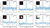 |
Fig. 1. F356W grism spectra for six Hα emitters in our sample. At the top of each panel, we report the stellar mass of the galaxy. The shaded region shows the uncertainty on the flux, and the 1.5″ × 1.5″ insets show false-color rest-frame optical RGB images constructed from NIRCam F115W/F200W/F356W. The green and brown lines highlight the Hαλ6564.6 and [N II] λλ6549.9, 6585.4 wavelengths, respectively. |
Since we are interested in star-forming galaxies, we removed 10 sources showing a broad or suspected broad Hα component (vFWHM > 1000 km/s) from our catalog (N = 605), see Table 4 of Matthee et al. (2025) for details on these objects.
In some cases, as a consequence of the adopted deblending parameter, galaxies are artificially split into multiple components during the SourceExtractor run. To avoid accounting multiple times for the same system, whose Hα-flux is blended in the grism data, we adopted a procedure similar to Matthee et al. (2023) and grouped sources below a certain angular separation and distance in redshift together. Specifically, we considered sources with |Δv|< 1000 km/s and angular separation < 0.8″(∼5.5 kpc at z = 4.3) as belonging to the same system and merged their physical properties (e.g., stellar masses and fluxes). This way we ensure that our selection criteria can be reproduced in galaxy simulations and that we are grouping together systems that belong to the same halo, for reference, the virial radius of a ∼1011 M⊙ halo at z = 4.5 is ∼30 kpc. The angular separation was chosen based on that of Covelo-Paz et al. (2025), where the authors used an angular separation < 0.6 arcsec (∼4.1 kpc at z = 4.3) for their NIRCam grism data, below which issues with blending may impact measurements. Since we consider objects in a lensed field, we multiply this separation value by the square root of the median magnification factor of the ALT Hα sample, μ = 1.95. Figure 2 shows the pair separation distribution function of the Hα emitters in ALT. All the above conditions lead to a sample of 512 objects, of which 61 (∼12%) are multicomponent galaxies.
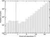 |
Fig. 2. Projected separation between all pairs of galaxies in our sample with Δv < 1000 km s−1. The dashed vertical line at 0.8″, which corresponds to ∼5.5 kpc at z = 4.3, is our choice for the maximum angular separation among components belonging to the same system. |
Finally, given the heterogeneity in the methods applied to identify our sample, as well as the wavelength-dependent sensitivity of our dataset, we decided to apply a conservative cut in the Hα flux and magnification to obtain a robust sample. Thus, we only consider galaxies with observed Hα fluxes larger than 10−18 erg s−1 cm−2, which allows for a 5σ line sensitivity in ALT6. This condition removes 74 galaxies from our sample. Moreover, to avoid being strongly affected by the magnification model, we restricted our sample to μ ≤ 2.5, which excludes 144 galaxies from our sample. We end up with a robust Hα sample of 316 objects with SNR ≳ 5, of which 43 (∼14%) consist of multiple components grouped together, that is, multicomponent galaxies. Although adopting a distance threshold to identify multicomponent galaxies may cause close pairs of compact merging systems to be treated as a single source, multicomponent galaxies constitute only 14% of the robust sample, and close mergers are expected to represent only a subset of these. Therefore, we do not expect the presence of close mergers in our sample to impact our results.
Figure 3 shows the observed Hα fluxes, not corrected for magnification, as a function of the spectroscopic redshift together with the redshift distribution of the Hα emitters. With our robust sample, we probed the entire redshift range of HAEs in ALT.
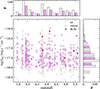 |
Fig. 3. Observed Hα fluxes as a function of redshift. We show the parent Hα sample (N = 512) in gray, and we highlight the robust sample in pink (N = 316, observed Hα flux > 10−18 erg s−1 cm−2 and μ ≤ 2.5). The red hexagons highlight the six confirmed broad-line Hα emitters (BLHα), with vFWHM > 1000 km/s, presented in Matthee et al. (2025). The hsistograms show the redshift and Hα flux distributions for the parent and robust samples. |
3. Methods
3.1. SED fitting
The physical properties of all galaxies in the ALT survey are estimated using the SED-fitting model Prospector (Leja et al. 2017, 2019; Johnson et al. 2021). All available photometry (JWST and HST, 27 bands) was used for the SED fitting, with the exception of filters that included the Lyα emission line and blueward because they are affected by the intergalactic medium. A detailed description of the adopted parameters can be found in Naidu et al. (2024). In short, we used stellar population models (Conroy & Gunn 2010; Conroy et al. 2009, 2010) that assume a Chabrier (2003) IMF and self-consistently include nebular emission modeled with Cloudy (Ferland et al. 2017) grids described in Byler et al. (2017). The parameters we fitted for include a non-parametric SFH, the total stellar mass, stellar and gas-phase metallicities, nebular emission parameters and a flexible dust model (Kriek & Conroy 2013).
For the SFH we adopt the “bursty continuity” prior of Tacchella et al. 2022a, with time bins logarithmically spaced up to a formation redshift of z = 20. The stellar and gas phase metallicities are not tied to each other and span log(Z/Z⊙) = −2 to 0.19 and −2 to 0.5 respectively. Dust attenuation has been modeled using a two-component dust attenuation model with flexible attenuation curve (Charlot & Fall 2000). This model accounts for a birth-cloud component that attenuates nebular and stellar emission from stars formed in the last 10 Myr and a diffuse component that has a variable attenuation curve (Kriek & Conroy 2013) and attenuates stellar and nebular emission from the galaxy (details on dust attenuation assumptions explained in Naidu et al. 2024; Tacchella et al. 2022a).
The dust correction at the Hα wavelength was derived by generating posterior SEDs by including the dust parameters and then by setting them to zero.
The emission line fluxes measured from the grism data are not included in the fitting procedure, as they are covered by medium-band photometry. For almost all sources, the photometry also covers the optical continuum which is free from emission-line contamination in various broad- and/or medium-band filters.
3.2. SFR estimates
In this work, we focus on star formation on short timescales (≤10 Myr), for which the nebular emission from Hα line is a particularly effective tracer.
The conversion from intrinsic Hα luminosity to SFR is typically derived using spectral synthesis models and depends on several assumptions, including IMF, star formation history, and stellar metallicity (Tacchella et al. 2022b). For example, stellar atmospheric temperatures, and hence the ionizing-photon output, depend on metallicity owing to line blanketing, that is, the absorption of high-energy radiation by metal lines in stellar atmospheres. A widely used calibration is that of Kennicutt (1998b, see also Kennicutt & Evans 2012) which assumes a constant SFH over t = 100 Myr and solar metallicity, based on the typical conditions in galaxies in the low-redshift Universe. While this calibration is commonly applied to high-redshift galaxies, it should be noted that such systems often have subsolar metallicity, which may affect its accuracy.
To compute the SFRs of the galaxies in our sample we used dust-corrected Hα luminosities. The relation between intrinsic Hα luminosity ( ) and SFR is as follows:
 (1)
(1)
where C is a metallicity and IMF dependent conversion factor (see the discussion in McClymont et al. (2025) and Kramarenko et al. (2026)). Following Theios et al. (2019, see also Clarke et al. 2024), we adopt C = −41.59, suitable for high-z galaxies (see, e.g., Shapley et al. 2023; Pollock et al. 2025). Estimates for the SFR are highly dependent on the assumed conversion factor which, in turn, depends on the assumed metallicity. By adopting a standard calibration from Kennicutt & Evans (2012), we would have predicted a factor ∼2× higher SFR values than our current estimates. This is because low-metallicity stars are hotter and have reduced line blanketing, both effects leading to greater ionizing photon output and, consequently, more Hα emission per unit SFR.
Equation (1) assumes that the LyC escape fraction ( ) is equal to zero, that is, all ionizing photons are absorbed by hydrogen in the ISM of the galaxy. Although this may not be true for all galaxies in our sample, only very large
  would affect our results. Mascia et al. (2023) and Giovinazzo et al. (2026) analyzed the JWST data (4.5 ≤ z ≤ 8) on A2744 finding
  or lower, corresponding to a correction factor of only ∼1.1.
Figure 4 shows the SFR–M★ plane for z = 3.7 − 5.1 probed by ALT compared to that of the Complete NIRCam Grism Redshift Survey (CONGRESS, Egami et al. 2023; Covelo-Paz et al. 2025). CONGRESS employs F356W grism in the GOODS-North field to perform a blind search for Hα emitters in the redshift range z = 3.7 − 5.1. Since ALT has significantly longer exposure time and observes galaxies behind the A2744 lensing cluster, we are able to access lower mass galaxies that extend the parameter space down a factor ∼30 to M★ ∼ 106 M⊙.
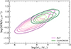 |
Fig. 4. Probed parameter space in the SFR–M★ plane. The parameter space probed by ALT (pink) compared to that of the CONGRESS survey (green). The two surveys cover Hα emission in the redshift range z = 3.7 − 5.1. CONGRESS (Egami et al. 2023; Covelo-Paz et al. 2025) employs F356W grism in the GOODS-North field and captures galaxies with a median stellar masses higher than those from ALT, while ALT extends the parameter space approximately 2 orders of magnitude lower in stellar mass. |
3.3. Bayesian model
We implemented a Bayesian model, using the Markov Chain Monte Carlo (MCMC) method7 to fit the relation between SFR and M★, while properly accounting for controlled observational selection effects. In this model, we parametrize the SFMS as a linear relation between SFR and M★ in log-log space. We include the intrinsic Gaussian scatter of the relation, which may be mass-dependent. Although previous works found evidence for a redshift-dependent flattening in the SFMS at high masses, leading to a different parameterization of this relation (e.g., Lee et al. 2015; Popesso et al. 2023), we adopt a linear relation since all galaxies in our sample lie below the characteristic mass ∼ 1011 M★ of the turnover at z ∼ 4.5. The relation we fit in the log-log space is
 (2)
(2)
In the following, α = ms_slope and β = ms_norm, which is the intercept at log(M★/M⊙) = 10.5. We use the notation 𝒩(0 , σint2) to indicate a Gaussian distribution with zero mean and variance σint2. The standard deviation, that is, intrinsic Gaussian scatter, σint, is assumed to be related to the stellar mass following a linear relation:
 (3)
(3)
The total observed scatter of the relation is defined as  where σobs accounts for the observational uncertainties. There are four key parameters in this model: (ms_slope, ms_norm) and (a, b). In Sect. 5.3 we test the effect of a non-Gaussian scatter around the SFMS, which accounts for the presence of a low-SFR tail at fixed stellar mass.
We compute the posterior likelihood using the probability function of the star formation rate (p). In particular, we model SFR distributions using truncated normal distribution functions centered on the SFR values calculated from Eq. (2), using the observed M★, with the total sigma (σ) as the standard deviation. The uncertainties on SFRs are assumed to be Gaussian and enters as σobs in the total sigma. Each Gaussian distribution is truncated to mimic the SFR-limited selection of our sample, resulting in the selection-corrected probability p. The truncation is defined using Eq. (1) with fHα = 10−18 erg s−1 cm−2 at fixed z = 5, which results in a conservative SFR cut in our sample. We refer to this model, schematically illustrated in Fig. 5 (top panel), as our reference model.
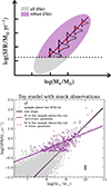 |
Fig. 5. Top: Model we used to describe the observed SFMS. The gray cloud represents all the HAEs in ALT, while the pink one is the observed sample after applying the selection criteria for robustness. Red points are the observed SFR, whose probability at fixed stellar mass is modeled using a truncated normal distribution that can be mass dependent. The normal distributions are centered in the SFR values predicted using the observed stellar masses and Eq. (2) whose parameters are explored within the MCMC sampling. Bottom: Toy model results. Mock observations generated sampling the stellar mass function from Weibel et al. (2024) with n_samples = 30 000. Gray dots show the entire sample, purple circles are galaxies with SFR > 0.7 M⊙/yr. The solid black line is the fit to the entire sample, while pink dashed and purple solid lines respectively show the fits with and without truncated normal distributions in the Bayesian model. The error bar in the bottom right is the 0.1 dex uncertainty on the SFR for each mock observation, corresponding to the average star formation rate uncertainty derived from observational data. |
To validate our model, we generate mock observations sampling the stellar mass function from Weibel et al. (2024, n_samples = 30 000) and the SFR–M★ relation with known input parameters (ms_slope = 1, ms_norm = 1.66 at log(M★/M⊙) = 10.5, a = −0.05 and b = 0.3 dex). From the total sample, we define the robust sample as the one with SFR > 0.69 M⊙/yr, derived from Eq. (1) with fHα = 10−18 erg s−1 cm−2 and z = 5. Based on the mean value of the uncertainties on the observed robust sample, we assumed Gaussian uncertainties for SFRs of 0.1 dex. Then, we fit the robust mock sample with and without truncated Gaussian distributions in our Bayesian model. Figure 5 (bottom panel) shows that without taking into account the selection effect the cutoff has on the sample, we would estimate a shallower slope of ms_slope = 0.40 ± 0.02 and, as a consequence, a smaller normalization (purple solid line). The slope, normalization and scatter-related parameters are recovered (ms_slope =  , ms_norm =
  ,
,  ,
,  ) once we account for the SFR cutoff and use truncated Gaussian distributions (pink dashed line).
We used this log-likelihood function as the objective function for MCMC parameter exploration, identifying the combinations of parameters (ms_slope, ms_norm, a, b) that best describe the observed sample by maximizing likelihood.
4. Results
4.1. Dust attenuation
Figure 6 shows the Hα obscured fraction, estimated using Prospector, as a function of stellar mass for the ALT robust sample. Despite significant scatter in the relation, we observe the trend of increasing dust attenuation with stellar mass. The Hα is heavily obscured (fobs > 50%) above the stellar mass of ∼6 × 10⁹ M⊙, however, most (95%) of the galaxies in our robust sample have an obscured fraction of Hα < 50%. Interestingly, due to the large scatter in fobs at all masses, there are galaxies with high dust obscuration even down at ∼4 × 10⁸ M⊙.
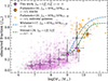 |
Fig. 6. Obscured star formation as a function of the stellar mass. The fraction of dust attenuated Hα emission, i.e., the ratio of the obscured and total Hα luminosity, as a function of stellar mass for the ALT sample. In gray is the parent Hα sample, while highlighted in pink is the robust one. Median values in each mass bin are shown as filled circles. Empty markers show obscured Hα fraction once we account for enhanced dust attenuation in high-mass galaxies (see Sect. 5.4). As a comparison, we show the fraction of obscured star formation for galaxies at 2 < z < 2.5 from Whitaker et al. (2017, blue), at 0.7 < z < 2 from Shivaei et al. (2024, green), and at z ∼ 4.5 ALPINE galaxies from Fudamoto et al. (2020, orange), with squares showing individual FIR continuum detections at 4 < z < 5 and triangles the 3σ upper limits for IR non detections. Filled squares show stacks in 2 mass bins at z ∼ 4.5. |
In Fig. 6 we show the fraction of obscured star formation (i.e., the fraction of star formation activity observable from IR continuum emission relative to its total amount) at 2 < z < 2.5 estimated by Whitaker et al. (2017) using Spitzer/MIPS observations of a mass complete sample at log(M★/M⊙) ≳ 9. The authors find that fobs is highly mass dependent, with more than 80% of star formation being obscured at log(M★/M⊙) ≳ 10 and that this relation does not evolve with redshift. In Whitaker et al. (2017), the authors discussed that for M★ < 1010 M⊙ the estimated IR luminosity systematically changes depending on the FIR SED template adopted. Their default template does not include an evolution of the dust temperature with redshift. More recently, Shivaei et al. (2024) studied the fraction of obscured UV emission using data from the Systematic Mid-infrared Instrument Legacy Extragalactic Survey (SMILES) (Alberts et al. 2024; Rieke et al. 2024) at z = 0.7 − 2. Shivaei et al. (2024) confirm a redshift-independent strong correlation between the dust-obscured fraction and stellar mass. Although the two relations agree relatively well, Shivaei et al. (2024) argue that the single FIR SED assumption in Whitaker et al. (2017) might have led to an overestimation of their IR luminosity values at lower masses and, as a consequence, of their obscured fraction. Furthermore, the different covered areas and the sensitivity of SMILES and Spitzer/MIPS may also play a role in the observed discrepancies between these two studies. SMILES is more sensitive to less obscured galaxies at fixed mass and covers a smaller area compared to Spitzer/MIPS.
Finally, we show the fraction of obscured star formation for galaxies from the ALMA Large Program to Investigate C+ at Early Times (ALPINE, Fudamoto et al. 2020). In particular, we show fobs for individual galaxies with and without IR detection and the results of stacks in two mass bins (M★ > 1010 M⊙ and M★ < 1010 M⊙). The stacks show a lower obscured fraction compared to Whitaker et al. (2017), but relatively good agreement with Shivaei et al. (2024). However, individual sources with IR detection agree well with both relations, highlighting an obscured star formation higher than 60%.
Notably, we find that the fraction of the obscured star formation rate of our robust sample is in agreement with the trend of Shivaei et al. (2024) for log(M★/M⊙) = 9 − 10.
4.2. The SFR–M★ relation
Figure 7 shows the SFMS at 4 < z < 5 with SFRs derived from Hα and that spans a mass range log(M★/M⊙) = 6.43 − 10.57. We show the entire (gray) and robust (pink) ALT Hα samples, together with the median values when binning in stellar mass. The errors on the medians come from bootstrapping with 300 realizations with replacement (16th and 84th percentiles) and bin sizes are chosen to ensure at least 13 galaxies in each bin. For the robust sample, we reach mass completeness above 90% for galaxies with log(M★/M⊙) > 8.5 (see Appendix A), shown with filled circles for the median values. For reference, we also show the SFMS trend from Speagle et al. (2014, together with its measured 0.3 dex scatter), Popesso et al. (2023), and Khusanova et al. (2021). The trend from Speagle et al. (2014), constrained from z ∼ 0 to z ∼ 5, is the result of a compilation of literature studies. Their galaxy sample has stellar masses down to 108 M⊙ and SFRs derived from the rest-frame UV continuum. Popesso et al. (2023), compiled more recent literature data to investigate the redshift evolution (0 < z < 6) of the SFMS. Most SFR estimates are based on UV+IR data or are derived through SED fitting techniques based on UV+IR from ground-based telescopes, HST and Spitzer. They probed the stellar mass range from 108.5 M⊙ to 1011.5 M⊙, highlighting the presence of a bending in the relation for large stellar masses, log(M★/M⊙) > 10.5. Finally, we show the SFMS fit from Khusanova et al. (2021), based on observations from ALMA-ALPINE (Faisst et al. 2020; Béthermin et al. 2020; Le Fèvre et al. 2020). These galaxies, at 4 < z < 5, have masses in the range 8.5 < log(M★/M⊙) < 11 and SFR estimates derived from rest-frame UV+IR information. All the above trends from literature studies, that based their SFR estimates on UV + IR data, show a slope of the SFR–M★ relation close to unity.
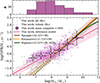 |
Fig. 7. SFR–M★ relation at 3.7 < z < 5.1. In gray is the entire ALT Hα sample, while highlighted in pink is the robust subsample. Circles show the median value when binning in stellar mass (upper panel). We are > 90% mass complete for galaxies with log(M★/M⊙) > 8.5 (filled circles). For reference, we show the SFMS fits by Speagle et al. (2014, together with its 0.3 dex scatter) and Popesso et al. (2023) from a compilation of literature observations and the fit by Khusanova et al. (2021) from ALMA-ALPINE observations. Dotted lines mark extrapolations to these relations based on their lower limits on M★. Solid pink line and shaded region denote respectively the best-fit line and 1σ interval about the SFMS using the reference model that accounts for the selection function (see Sect. 3.3). |
Median Hα-based SFRs in stellar mass bins in the ALT sample at z = 3.7 − 5.1.
Figure 7 shows that for stellar masses above log(M★/M⊙) = 8.5 our Hα derived main sequence agrees well with that derived from the rest-frame UV and UV+IR continuum at z = 4.5. Going toward lower stellar masses, we find a flattening in the data points mainly driven by the selection effect on the Hα flux, which biases our observed sample (i.e., flux-limited survey). Indeed, because of the widely varying luminosities and faintness of low-mass galaxies, it is difficult to obtain complete samples at a given mass. As a consequence, the selection of galaxies near the flux limit results in a biased sample toward galaxies in the burst phase (Malmquist bias; see Reddy et al. 2012). Moreover, we measure an intrinsic scatter σint ∼ 0.32 dex at log(M★/M⊙) = 8, consistent with the scatter reported by Smit et al. (2016) at z ∼ 4 − 5 and that of Shivaei et al. (2015) at z ∼ 2 for higher stellar masses, which are both based on Hα observations. This scatter is slightly larger than the 0.3 dex estimated by Speagle et al. (2014), using UV + IR data. Such a dispersion in the robust data sample is not unexpected and can be attributed to bursty star formation histories traced using Hα emission line (e.g., Domínguez et al. 2015; Faisst et al. 2019; Caplar & Tacchella 2019; McClymont et al. 2025). However, as argued by Shivaei et al. (2015), without direct measurements of galaxy-to-galaxy variations in attenuation curves and the IMF, differences in the scatter between the SFR(Hα)–M★ and SFR(UV)–M★ relations cannot be reliably used to constrain the stochasticity of star formation in high-redshift galaxies.
Using a simple linear fit with scipy.curvefit applied to our robust sample of HAE, we derive a SFMS slope of ms_slope = 0.45 ± 0.02, consistent with other JWST/NIRSpec measurements (e.g., Chemerynska et al. 2024), and a normalization of 1.26 ± 0.06 M⊙ yr−1 at log(M★/M⊙) = 10.5. However, as the ALT survey is a flux-limited survey, our low-mass sample is biased toward galaxies with higher specific SFRs as illustrated in Fig. 5.
In order to fit the observational sample taking into account its biased nature, we employ the Bayesian model described in Sect. 3.3 assuming uniform prior probability distributions, with each parameter restricted to the range: ms_slope =[0.2, 1.8], ms_norm =[0.01, 2.4], a = [ − 0.1, 0.3], b = [0.1, 1.3]. We used Bayesian inference through MCMC sampling, using the autoemcee Python package, to explore the parameter space and determine posterior distributions for the parameters. The solid line and shaded region in Fig. 7 show the best-fit model and 1σ interval when applying our reference model to the robust Hα sample from ALT. We list the median SFRs in stellar mass bins in Table 1, as well as the estimated stellar mass completeness of the galaxy sample in each mass bin (see Appendix A).
Figure 8 presents the corner plot for the inferred posterior distributions for the parameters explored in our model: the slope and normalization of the SFMS (ms_slope, ms_norm) and the slope and normalization of the intrinsic scatter (a, b) – see Eqs. (2) and (3). The three panels in the upper right corner show the mass evolution of σint, derived using the posterior distributions for a and b together with Eq. (2). From the corner plot, we observe a strong positive correlation between ms_slope and ms_norm, reflecting the slope-intercept degeneracy that arises when fitting linear relations. The positive correlation between the scatter parameters (b – a) also highlights that the intrinsic scatter normalization and its mass dependence are degenerate. Table 2 reports the median value of the MCMC sample distribution and the 16th and 84th percentiles (i.e., 1σ confidence interval). The median posterior parameters, which are consistent with the best-fit values, suggest a steeper slope (ms_slope  ) than that of curvefit and a normalization of 1.44 ± 0.15 M⊙ yr−1 at log(M★/M⊙) = 10.5. Although the slope is consistent with that reported by Shivaei et al. (2015) for Hα emitters at z ∼ 2, it is shallower than that derived from UV+IR data (e.g., Popesso et al. 2023). In the literature, some studies report constant scatter (e.g., Clarke et al. 2024), while others find evidence for mass-dependent variation (e.g., Domínguez et al. 2015; Santini et al. 2017; Cole et al. 2025; Clarke et al. 2025). In our analysis, we find an intrinsic scatter that slightly increases with stellar mass (inset panels, Fig. 8). This is suggested by the positive value assumed by a, which controls the mass dependence of the intrinsic scatter. However, the large 1σ uncertainty associated with this parameter prevents us from drawing strong conclusions about the mass dependence of the scatter.
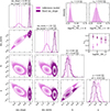 |
Fig. 8. Output of our reference model. Corner plot and posterior distributions (pink) of the four key parameters in our reference model: SFMS slope and normalization at log(M★/M⊙) = 10.5 (ms_slope, ms_norm) and the slope and normalization of the intrinsic scatter (a, b). The contours show the 1σ, 1.5σ, and 2σ confidence levels. We adopted truncated normal distributions to model the SFRs distribution in our Bayesian model (see Sect. 3.3). In purple we show the posterior distributions after running the Bayesian model on the robust sample imposing a Gaussian prior (mean = 1 and σ = 0.02) on ms_slope, referred to as “fixed ms_slope” in the legend. Above each panel we report medians with uncertainties (16th and 84th percentiles), those with asterisks refer to fixed ms_slope. The inset panels on the right show the intrinsic scatter distributions at two stellar masses, computed combining the posterior distributions for a and b with Eq. (2), and the σint evolution with stellar mass for the reference model and the model with a fixed ms_slope. |
4.3. Comparison with other observations
In Fig. 9, we compare the SFMS of our robust Hα sample with that of samples in the literature (Covelo-Paz et al. 2025; Clarke et al. 2024; Faisst et al. 2019; Sun et al. 2025). We binned in mass the available observations to compute the medians and 1σ uncertainties by bootstrapping, where we resample our galaxies with replacements 300 times. The SFR values in CONGRESS (Covelo-Paz et al. 2025), and in the JWST Advanced Deep Extragalactic Survey (JADES) and the Cosmic Evolution Early Release Science Survey (CEERS) (Clarke et al. 2024) data have been derived using the same conversion between LHα and SFR as in this work, while those of ALPINE (Faisst et al. 2020) and ASPIRE (Sun et al. 2025) are estimated using SED fitting codes, including information from the FIR part of the spectrum in the fit. For all the datasets, stellar masses were estimated from SED fitting codes, and all IMFs were converted to a Chabrier IMF for consistency. To guide the eye, we show a linear relation with a slope of one, generally predicted by simulations and theoretical models, and an arbitrary normalization to highlight the flattening present in the observational data in the low stellar mass range (log(M★/M⊙)≲8.5), above which our sample is > 90% mass complete (see Appendix A).
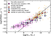 |
Fig. 9. Comparison with literature studies in the redshift range 4 < z < 5. The robust Hα sample used in this work and its binned values are in pink circles, blue and green triangles are mass binned observations from CONGRESS (Covelo-Paz et al. 2025) and, CEERS and JADES JWST-surveys (Clarke et al. 2024), respectively. Orange squares show observations from ALMA-ALPINE (Faisst et al. 2020), while the red square is the binned value for the ASPIRE survey which combines JWST and ALMA observations (Sun et al. 2025). To guide the eye, we show a linear relation with slope one (dashed black). |
Overall, we find good agreement between the trend identified in this work and that from literature observations, despite the caveats arising from the diverse assumptions adopted in SED fitting (e.g., dust attenuation laws and star formation histories). In particular, we find better agreement with JWST-only observations (CEERS+JADES and CONGRESS), whereas our results tend to fall slightly below the SFR predictions from ALPINE, which include ALMA observations and primarily probe the high-mass end of the relation, where our statistics are limited. The discrepancy with ALPINE data may arise from (i) the incompleteness of the ALPINE sample for stellar masses M★ < 109 M⊙; (ii) potential underestimation of dust content in massive galaxies within our sample. We have few sources covering the mass range probed by the ASPIRE survey, which has observation made with JWST/NIRCam WFSS in the F356W (along with imaging in F115W, F200W and F356W) and with ALMA 1.2 mm continuum. However, when we consider the CONGRESS survey – which, like ALT, lacks information from the FIR part of the spectrum and relies solely on JWST/NIRCam grism and imaging, but extends to higher stellar masses – we find that it predicts systematically lower star formation rates. This discrepancy may be due to an underestimation of dust attenuation in CONGRESS, which could suggest a similar effect in ALT (see Sect. 5.4).
The comparison with literature data highlights the high number statistics of ALT galaxies at the low-mass end of the SFR–M★ relation: 54% of the robust Hα sample has log(M★/M⊙) < 8. By adequately accounting for the selection bias that affects our dataset, we allow for a population-level analysis at 4 < z < 5 based on a spectroscopic sample that covers the region of the SFR–M★ plane below log(M★/M⊙) < 7.5. This part of the plane has remained largely unexplored to date; however, see Rinaldi et al. (2022) where the authors analyzed a Lyman-α selected sample of galaxies in the blank and lensed fields reaching the low-mass end of the SFMS.
5. Discussion
5.1. A flat main-sequence slope?
In order to interpret our results, we perform detailed comparisons to hydrodynamical simulations, mimicking, as much as possible, the techniques adopted for the observational sample. Hydrodynamical simulations report a unitary slope for the SFR–M★ relation that does not evolve with redshift (e.g., Pillepich et al. 2019; Di Cesare et al. 2023; Katz et al. 2023; Furlong et al. 2015; McClymont et al. 2025).
Figure 10 shows the posterior distributions obtained by applying the Bayesian model (Sect. 3.3) to the robust ALT sample as well as to the data from hydrodynamical simulations at z ∼ 4.5. We consider data from dustyGadget (Graziani et al. 2020), EAGLE (Schaye et al. 2015; Crain et al. 2015), Illustris-TNG50 (Pillepich et al. 2019), SPHINX20 (Rosdahl et al. 2018, 2022) and THESAN-ZOOM (Kannan et al. 2025; McClymont et al. 2025) simulations. In particular, the samples used in the Bayesian model consist of stellar masses and star formation rates in each simulation. We apply a SFR cutoff to these simulated galaxy samples, similar to what we do for the observed sample. The specific value of the SFR cutoff varies across simulations, depending on factors such as the number of galaxies remaining after the cut (to ensure a statistically meaningful sample) and properties of each simulation, for instance, the SPHINX20 data release has a built-in SFR threshold.
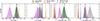 |
Fig. 10. Comparison between our inferences from observations and hydrodynamical simulations. Posterior distributions for the slope, normalization and intrinsic scatter of the SFMS. We compare the posteriors based on the ALT robust Hα sample (pink, hatched) explored in this work with those from dustyGadget (brown; Graziani et al. 2020; Di Cesare et al. 2023), EAGLE (blue; Schaye et al. 2015; Crain et al. 2015), IllustrisTNG-50 (orange; Pillepich et al. 2019; Nelson et al. 2019), SPHINX (green; Rosdahl et al. 2018, 2022; Katz et al. 2023) and THESAN-ZOOM (gray; McClymont et al. 2025) simulations. |
These simulations adopt different numerical strategies and physical assumptions, such as feedback schemes and ISM models, as well as varying mass resolutions and box sizes. For reference, EAGLE has a side length of 100 cMpc, dustyGadget’s side length is 74 cMpc, Illustris-TNG50 span 50 cMpc, and SPHINX covers 20 cMpc, while THESAN-ZOOM is a high-resolution zoom-in simulation targeting galaxies selected from the THESAN parent volume (95.5 cMpc, Kannan et al. 2022). Importantly, mass resolution and box size are not independent: larger volumes typically come at the expense of lower mass resolution. While larger simulation boxes allow for better statistics and sampling of massive galaxies, their lower mass resolution prevents them from resolving low-mass systems (e.g., log(M★/M⊙) < 8). This trade-off also extends to the ISM modeling. Simulations with coarser resolution (often those with larger volumes) tend to adopt averaged or subgrid ISM models, while higher-resolution simulations can implement more detailed, multiphase ISM treatments that better capture the structure and physics of the star-forming gas.
The first two panels of Fig. 10 show that: (i) the best-fit values for the ms_slope in simulations are ∼1 and are consistent among all of them; (ii) the slope is found to be shallower in our observations; (iii) the ms_norm at log(M★/M⊙) = 10.5 increases with the steepness, as a consequence of the slope-normalization degeneracy. Finally, the last two panels show an increasing intrinsic scatter σint with stellar mass from our observations, whereas simulations show either a scatter that decreases with mass (dustyGadget, SPHINX) or a mass-independent behavior (IllustrisTNG-50, EAGLE). Interestingly, we find that the intrinsic scatter increases with stellar mass in the THESAN-ZOOM simulations. This may be due to the fact that, as zoom-in simulations, THESAN-ZOOM has a lower statistics at high-stellar masses (log(M★/M⊙) > 10). Except for SPHINX and THESAN-ZOOM, all simulations show lower values of σint at log(M★/M⊙) = 8 compared to observational data. This discrepancy among simulations likely arises from the resolution of each simulation and the way in which star formation and feedback mechanisms are implemented within simulation schemes. These physical processes are known to drive stochastic variations in star formation (e.g., Matthee & Schaye 2019), and the inability to resolve such processes in simulations may dampen the variability of star formation histories. This interpretation is supported by the fact that SPHINX and THESAN-ZOOM, which uses the smallest simulation boxes, thus the highest resolution, have the largest σint (∼0.47 dex) at log(M★/M⊙) = 8. Moreover, these two simulations implement the detailed physics of a multiphase ISM (Katz et al. 2023; Kannan et al. 2025).
It is also worth noting that different simulations trace star formation on different timescales. While for SPHINX and THESAN-ZOOM we consider SFR averaged over 10 Myr, for Illustris-TNG, dustyGadget and EAGLE we use instantaneous SFR estimates. Note that Pillepich et al. (2019) found that the scatter in TNG50 is constant regardless of the way SFR is measured (i.e., instantaneous or averaged over 10 or 100 Myr). The median values of the posterior distributions for each parameter are presented in Table 2.
Comparison with SFMS trends from literature observations (Fig. 7) and simulations (Fig. 10) highlights a shallow slope (ms_slope ∼0.59) for the Hα ALT robust data sample. This slope is inconsistent with predictions from hydrodynamical simulations, and also with theoretical expectations based on the stellar mass function. Leja et al. (2015) demonstrate that a simple extrapolation of the SFMS trend8 from Whitaker et al. (2012) to low-mass galaxies (down to 109 M⊙) would over-predict the number density of galaxies at z ∼ 2 by factor 100 (their Fig. 3), see also Peng et al. (2014). This growth is the result of the relatively flat slope of the star-forming sequence. The authors argue that the rate of merger interaction cannot compensate for the rapid growth of low-mass galaxies implied by such flat slopes (see also Fu et al. 2024). If we apply the same logic at z ∼ 4.5, a slope of  , through the relation between the SFMS and the SMF, would imply a steepening at the low-mass end of the stellar mass function, which is not supported by observations (e.g., Weibel et al. 2024).
To investigate the impact of a steeper slope on the posterior distributions of the estimated parameters, we reran the Bayesian model on the robust observational sample, imposing a narrow Gaussian prior on the ms_slope parameter (mean = 1, σ = 0.02), strongly constraining it to values near unity. In this case, we find an increase in the ms_norm along with an intrinsic scatter which decreases with stellar mass, more in line with simulations. The intrinsic scatter values are approximately σint ∼ 0.49 dex at log(M★/M⊙) = 8 and σint ∼ 0.40 dex at log(M★/M⊙) = 10, as illustrated in Fig. 8 (purple). Interestingly, this indicates that with our robust sample it is challenging to simultaneously constrain the slope and the scatter dependence on mass. However, once we fix one parameter (e.g., the slope), we can fit the mass-dependence of the scatter, which decreases with increasing stellar mass.
5.2. Testing the effect of varying SFR calibrations
The slope of the SFMS depends on the star formation rate calibrations, which are sensitive to several galaxy properties such as the nature of the massive stellar population (including the role of binary stars), the ISM conditions (i.e., stellar metallicity and dust attenuation), and the assumed IMF (e.g., Kennicutt 1998a; Kennicutt & Evans 2012; Theios et al. 2019). In this section we investigate how different SFR calibrations affect the best-fit parameters constrained by our reference model.
Generally, literature calibrations assume a linear relation between the Hα luminosity and the SFR, with a constant conversion value (C). Recently, Kramarenko et al. (2026) analyzed SPHINX20 simulations at 4.64 ≤ z ≤ 10. Using the simulated galaxy data from SPHINX20 they selected a sample of star-forming galaxies representative of the Hα population observed with JWST at high-redshift. They found that due to the metallicity dependence of the SFR–LHα relation, the classical calibrations (e.g., Kennicutt 1998a), on average, overestimate the SFRs of faint galaxies in SPHINX by SFR(Hα)/SFR10 ≳ 0.1 dex. The authors propose two new calibrations: one SFR(Hα) calibration that depends only on intrinsic Hα luminosity (Eq. (4)) and the other that additionally depends on the Hα equivalent width (Eq. (5)), a parameter that is sensitive to stellar metallicity and age,
 (4)
(4)
and
 (5)
(5)
where EW0,Hα is the rest-frame equivalent width of the Hα emission line.
We calculate SFRs for the ALT robust Hα sample using the alternative calibrations from Kramarenko et al. (2026) and derive new median posteriors with our reference model. Figure 11 compares the resulting posterior distributions, and Table 2 summarizes the median posterior parameters for slope, normalization, and intrinsic scatter parameters.
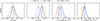 |
Fig. 11. Effect of the new luminosity and EW-dependent SFR(Hα) calibrations. Comparison of the posterior distributions for the slope, normalization and intrinsic scatter of the observed SFMS, adopting diverse LHα–SFR conversions. In pink are those derived using the calibration from Theios et al. (2019) (ref.), in blue and yellow are the distributions using calibrations based on SPHINX simulations (Kramarenko et al. 2026). Specifically, in blue we show the posteriors derived from calibrations based on LHα of the galaxies, while in yellow those combining the information from LHα with that from the EWHα. |
These alternative calibrations produce slightly steeper slopes (up to 14% increase) and correspondingly higher normalizations. Specifically, using the calibration in Eq. (4), we find ms_slope = 0.66 ± 0.08 and ms_norm = 1.79 ± 0.14 M⊙ yr−1, while with that in Eq. (5) we derive ms_slope = 0.67 ± 0.05 and ms_norm = 1.95 ± 0.11 M⊙ yr−1. The intrinsic scatter shows calibration-independent behavior, remaining approximately constant throughout the explored mass range.
5.3. Testing the effect of a non-Gaussian scatter
In our reference model, we adopted truncated normal distributions to model the SFMS scatter accounting for selection effects in our flux-limited sample. However, McClymont et al. (2025) demonstrate, using THESAN-ZOOM simulations (Kannan et al. 2025), that SFRs at fixed mass deviate from log-normal distributions and show a long tail down to zero (see also Feldmann 2017, 2019). Such a tail, particularly evident at the low-mass end of the relation, may stem from the presence of (mini-) quenched galaxies, systems in which star formation is halted or strongly suppressed (Dome et al. 2024; Looser et al. 2025; Gelli et al. 2025), that populate the lower portion of the SFR–M★ parameter space.
To investigate the impact of the presence of a low-SFR tail in the SFMS, we modified our reference model to account for a skewed intrinsic scatter, truncated below a threshold value to account for our flux-limited sample selection. We refer to this formulation as the non-Gaussian model. Details can be found in Appendix B.
Since the values of the skewness parameter (a_skew) are unknown, we treat it as a free parameter when applying this model to SPHINX and THESAN-ZOOM data. Then, we used a_skew estimates from simulations as Gaussian priors for this parameter and fit the Hα robust observations. We selected data from SPHINX and THESAN-ZOOM as these are the two simulations with higher resolution and smaller boxes, which give insights into the scatter at the low-mass end, where we expect (mini-) quenched galaxies to be.
By fitting SPHINX (THESAN-ZOOM) data with the non-Gaussian model, we derived values of a_skew =  (a_skew =
  ). These negative values of a_skew indicate a distribution skewed toward lower SFRs. We adopt these median values and their 1σ uncertainties as Gaussian priors in our non-Gaussian model to fit the ALT Hα robust sample. With priors from SPHINX data, we find a slope of ms_slope =
  . This result is consistent with the result from THESAN-ZOOM data, indicating that variations in a_skew have minimal impact on the slope. Moreover, its agreement with the reference Gaussian model shows that introducing skeweness in the SFR does not significantly affect the slope of the SFR–M★ relation.
5.4. Testing the effect of dust correction in high-mass galaxies
In this section we employ a simplified toy model to investigate how a potential underestimation of the dust obscuration at the high-mass end of the SFMS influences the inferred slope and scatter. Figure 6 presents a comparison between the fraction of obscured Hα emission in the ALT robust sample and that of obscured star formation and UV emission reported in the literature (Whitaker et al. 2017; Fudamoto et al. 2020; Shivaei et al. 2024). Whitaker et al. (2017) found a strong dependence of the median fobscured on stellar mass, with little evolution across the redshift range analyzed 0 < z < 2.5 (see also Shivaei et al. 2024). Moreover, they concluded that the transition from mostly unobscured to obscured (fobscured = 0.5) star formation occurs at stellar masses log(M★/M⊙) = 9.4.
To obtain a fiducial estimate of the potentially underestimated attenuation correction, we implement a mass-dependent dust obscuration correction designed to match the data from Whitaker et al. (2017) and observations from Fudamoto et al. (2020). This approach is motivated by observational evidence that more massive galaxies tend to have higher dust content and more complex dust geometries (e.g., Whitaker et al. 2017; Reddy et al. 2025). However, this method has several caveats. First, we compare the obscured dust fraction inferred from Hα emission with that derived from UV emission and UV-based star formation rates. This implicitly assumes that the ratio of the stellar and nebular extinction is unity at these redshifts and that the attenuation curves at optical and UV wavelengths are comparable. While these assumptions do not strictly hold, they are adopted here for the sake of illustrating the behavior of our toy model. Second, the model is calibrated to match the obscured fractions reported by Whitaker et al. (2017), although Shivaei et al. (2024) argue that these values may be systematically overestimated. We acknowledge these limitations and emphasize that this exercise is intended solely as a simplified demonstration to explore the qualitative effects of underestimated dust corrections.
For our toy model, we adopt a sigmoid function to represent a smooth, continuous transition in the strength of the dust correction as a function of stellar mass,
![Mathematical equation: $$ \begin{aligned} \omega (M_\star ) = \frac{1}{1 + \exp [s \times (M_\star - M_{\rm center})]}, \end{aligned} $$](/articles/aa/full_html/2026/03/aa57790-25/aa57790-25-eq69.gif) (6)
(6)
where M★ = log(M★/M⊙), Mcenter = log(Mcenter/M⊙) is the mass at which the weight equals 0.5 and s is the steepness parameter controlling the sharpness of the transition. We adopt Mcenter = 9.5 and s = 5, consistent with a rapid transition around the stellar mass value where dust obscuration becomes significantly important. We decrease the Hα transmission factor by feff where feff = 1 + (1 − ω)×(f − 1) is the effective correction factor, (1 − ω) is the inverted sigmoid weight that increases with stellar mass, and f is the factor by which the transmission is reduced for the most massive galaxies. We tested correction factors ranging from f = 1 (no correction) to f = 2 (reducing transmission by half) in steps of 0.2, finding that f = 2 is needed to reproduce the obscured faction curve of Whitaker et al. (2017), see empty markers in Fig. 6.
We apply these updated dust corrections to the observed Hα luminosities, after correcting for magnification, to recover intrinsic luminosities, and then compute SFRs using the calibration from Theios et al. (2019, our Eq. (1)). We then fit this updated sample with our Bayesian model and find a slope of ms_slope =  , together with an increase in normalization, as a consequence of the slope-intercept degeneracy. The intrinsic scatter remains consistent within the uncertainties across the stellar mass range, suggesting only a mild dependence on stellar mass. The median values of the posterior distributions for the parameters, which are consistent with the best-fit values, are summarized in Table 2.
While the implementation of enhanced dust attenuation corrections for high-mass galaxies – calibrated to match observed obscured star formation fractions from the literature – yields a steeper SFMS slope relative to the ms_slope obtained from our reference model, we caution that this result is subject to several assumptions. However, we likely underestimate contributions from optically thick star-forming regions, especially in massive galaxies. This bias may explain the comparatively shallower slope we obtain relative to studies incorporating IR emission. Future testing of this hypothesis can be pursued not only through ALMA observations in the IR, but also via JWST/MIRI measurements of Paschen recombination lines, which are less affected by dust attenuation than the commonly used Balmer lines.
5.5. How to reconcile SFMS observations with models?
In the previous sections, we tested and discussed several scenarios that may help reconcile the tension between our measured (flat) slope of the SFMS and the steeper slopes predicted by theoretical models and hydrodynamical simulations. Such reconciliation is necessary to reliably constrain the mass dependence of the scatter in the SFMS. Specifically, we investigated three key effects: a luminosity-dependent SFR(Hα) calibration, the presence of a ‘fat-tail’ of galaxies with low SFRs (i.e., non-Gaussian scatter), and the potential underestimation of obscured star formation in our observed sample. Although the first two primarily influence the low-mass end of the SFR–M★ relation, the third predominantly affects high-mass galaxies. These scenarios impact different aspects of our analysis: some modify the observational measurements (e.g., dust corrections or the conversion of Hα luminosity to SFR), while others affect the modeling within our Bayesian framework (e.g., incorporating non-Gaussian scatter).
We found that i) implementing new luminosity-dependent SFR(Hα) estimates based on SPHINX, with information on EW(Hα), results in a slightly steeper SFMS slope and an intrinsic scatter of ∼0.3 dex that is independent of stellar mass; ii) adopting a model that allows for non-Gaussian scatter around the SFMS does not significantly affect the slope of the relation. However, the intrinsic scatter shows higher median values as a function of stellar mass, albeit with increased uncertainties; iii) accounting for potentially underestimated dust attenuation in high-mass galaxies (log(M★/M⊙) > 9), yields a steeper ms_slope compared to the reference model and lower median values of the intrinsic scatter with little mass dependence. Among these tests, dust corrections have the strongest impact on the steepness of the SFR–M★ relation. However, none of these effects alone fully resolves the tension with theoretical models and predictions, suggesting that a combination of all these effects is needed to address this discrepancy.
Follow-up observations of our sample will enable us to observationally test the impact of each proposed effect. In particular, JWST/MIRI, NIRSpec and ALMA observations will allow us to search for characteristic spectral features that relate to the three scenarios presented in this work. JWST/NIRSpec observations of spectral features such as the intensity of the Balmer break and the presence (or not) of emission lines such as Hβ and [O III], along with measurements of their equivalent widths, would help us to identify (mini-)quenched galaxies, which would quantify the extent of non-Gaussian scatter, and constrain galaxy metallicity. Spectroscopy spanning rest-frame UV and rest-frame optical wavelengths would provide information on galaxies’ SFH which, combined with metallicity measurements, would allow us to test the luminosity-dependent conversion factors found in simulations. Detection of high-SNR Balmer lines would allow for more precise constraints on the Balmer decrement, leading to more accurate estimates of dust attenuation. Combined with JWST/NIRSpec spectroscopy and MIRI coverage of the Paschen recombination lines, ALMA observations of the IR emission from galaxies in our sample would provide complementary constraints on dust-obscured star formation.
6. Summary
We studied the relation between the SFR and M★ in the redshift range 3.7 < z < 5.1 using JWST/NIRCam grism data from the ALT survey. We focused on a robust sample of 316 Hα emitters in the region behind the lensing cluster Abell 2744, all with magnification factors μ ≤ 2.5. The stellar masses were derived through an SED fit based on all the medium- and broad-band filters available in this field. Notably, 54% of the galaxies in our robust sample have log(M★/M⊙)≤8, which enabled us to probe the low-mass end of the SFMS with a statistical sample. The star formation rates were estimated based on the Hα luminosity, and we adopted the calibration from Theios et al. (2019). We further examined how alternative calibrations based on predictions from a hydrodynamical simulation affected the inferred slope, intrinsic scatter, and normalization of the SFMS. Our observational sample is biased (i.e., flux-limited survey) toward brighter objects particularly in the low-mass end, and we therefore developed a Bayesian model for our analysis of the SFMS that accounted for the selection effect. Our main results are summarized below.
-
Using our reference model, we found a slope for the SFMS of ms_slope =
 , which is shallower than the slope based on literature data (e.g., Speagle et al. 2014; Popesso et al. 2023) and than the slope predicted by hydrodynamical simulations (e.g., Crain et al. 2015; Pillepich et al. 2019; Katz et al. 2023; Di Cesare et al. 2023; McClymont et al. 2025). The reference model yields intrinsic scatter of 0.3 dex at log(M★/M⊙) = 8 for the star-forming sequence, which slightly increases with stellar mass (see also Cole et al. 2025).
 -
By fixing the slope of the SFMS to unity, as predicted by theoretical models and simulations, we found the normalization to be ms_norm = 2.09−0.07+0.06 at log(M★/M⊙) = 10.5 and the intrinsic scatter to decrease with increasing stellar mass (see Fig. 8). In particular, σint = 0.46 ± 0.03 dex at log(M★/M⊙) = 8 and σint = 0.41 ± 0.07 dex at log(M★/M⊙) = 10 (see Fig. 8).
-
We compared the SFRs and stellar masses of the ALT sample with those of other JWST and ALMA surveys at z ∼ 4 − 5, finding a general good agreement. The high-mass end of the ALT data sample falls slightly below the SFR predictions of ALPINE and ASPIRE (Faisst et al. 2020; Sun et al. 2025), which both include ALMA observations. This discrepancy might arise from a potential underestimation of the dust content in the massive galaxies within our sample. If this is the case, massive galaxies in our sample would have higher SFR estimates, which would affect the slope of the SFMS.
-
We explored alternative SFR calibrations based on the SPHINX simulation (Eqs. (4) and (5), Kramarenko et al. 2026). We found that Eq. (5), which includes information on the EW, yields a steeper slope for the SFMS ms_slope = 0.67−0.05+0.06 and an intrinsic scatter of ∼0.35 dex that is roughly independent of stellar mass.
-
Following simulation predictions (e.g., McClymont et al. 2025), we investigated the possibility that the scatter around the SFMS might be non-Gaussian due to a population of galaxies that are relatively inactive. To explore this, we implemented skewed-normal distributions to model SFRs at fixed stellar masses within our Bayesian framework. We used data from the SPHINX and THESAN simulations to constrain the skewness parameter. We consistently found a_skew < 0, which indicates a distribution with a tail that extends toward lower SFR values. We adopted this simulation-derived skewness as a prior when we applied the non-Gaussian model to the ALT robust sample. While this approach yields a slightly steeper slope, ms_slope
 , than our reference Gaussian model, the difference is modest. This indicates that the skewness we introduced in the SFR does not substantially affect the overall SFR–M★ relation.
 -
We tested the effect of dust attenuation in high-mass galaxies on the slope of the SFMS by implementing a mass-dependent dust correction designed to reproduce the obscured fraction reported by Whitaker et al. (2017, see our Fig. 6). These updated attenuation values were applied to the observed Hα luminosities to derive revised SFRs (Eq. (1)). We then fit this updated dust-corrected sample using our reference Bayesian model, which accounts for the survey selection function. The resulting slope of the SFMS, ms_slope =
 , is steeper than that obtained from the original ALT Hα robust sample.
Although current data prevent simultaneous constraints on the slope and the mass-dependent nature of the scatter of the SFMS, our analysis showed that meaningful constraints can be drawn when one of the two is fixed to a known value from independent data. Our analysis underscored the importance of accounting for selection effects that shape observed galaxy samples. Additionally, we proposed several testable hypotheses, such as luminosity-dependent SFR calibrations, a population of low-mass mini-quenched galaxies, and a systematic underestimation of dust attenuation in high-mass systems. These hypotheses are crucial for robustly characterizing the mass dependence of the scatter and the (burstiness of) star formation histories in high-redshift galaxies.
Acknowledgments
We thank the anonymous referee for the insightful comments that helped improving the manuscript. We thank Romain. A. Meyer for valuable discussion, Pierluigi Rinaldi for his help with data handling and Luca Graziani and William McClymont for providing the dustyGadget and THESAN-ZOOM data, respectively. Funded by the European Union (ERC, AGENTS, 101076224). Views and opinions expressed are however those of the author(s) only and do not necessarily reflect those of the European Union or the European Research Council. Neither the European Union nor the granting authority can be held responsible for them. This work is based on observations made with the NASA/ESA/CSA James Webb Space Telescope. The data were obtained from the Mikulski Archive for Space Telescopes at the Space Telescope Science Institute, which is operated by the Association of Universities for Research in Astronomy, Inc., under NASA contract NAS 5-03127 for JWST. These observations are associated with program # 3516. We acknowledge funding from JWST program GO-3516. Software used in developing this work includes: matplotlib (Hunter 2007), numpy (Oliphant 2007), scipy (Virtanen et al. 2020), TOPCAT (Taylor 2005), and Astropy (Astropy Collaboration 2013).
References
- Abell, G. O., Corwin, H. G., Jr, & Olowin, R. P. 1989, ApJS, 70, 1 [Google Scholar]
- Abramson, L. E., Gladders, M. D., Dressler, A., et al. 2016, ApJ, 832, 7 [NASA ADS] [CrossRef] [Google Scholar]
- Alberts, S., Lyu, J., Shivaei, I., et al. 2024, ApJ, 976, 224 [Google Scholar]
- Astropy Collaboration (Robitaille, T. P., et al.) 2013, A&A, 558, A33 [NASA ADS] [CrossRef] [EDP Sciences] [Google Scholar]
- Bertin, E., & Arnouts, S. 1996, A&AS, 117, 393 [NASA ADS] [CrossRef] [EDP Sciences] [Google Scholar]
- Béthermin, M., Fudamoto, Y., Ginolfi, M., et al. 2020, A&A, 643, A2 [Google Scholar]
- Bezanson, R., Labbe, I., Whitaker, K. E., et al. 2024, ApJ, 974, 92 [NASA ADS] [CrossRef] [Google Scholar]
- Bhagwat, A., Costa, T., Ciardi, B., Pakmor, R., & Garaldi, E. 2024, MNRAS, 531, 3406 [NASA ADS] [CrossRef] [Google Scholar]
- Bollo, V., González, V., Stefanon, M., et al. 2023, ApJ, 946, 117 [NASA ADS] [CrossRef] [Google Scholar]
- Bouwens, R. J., Illingworth, G. D., Oesch, P. A., et al. 2015, ApJ, 803, 34 [Google Scholar]
- Bouwens, R. J., Oesch, P. A., Illingworth, G. D., Ellis, R. S., & Stefanon, M. 2017, ApJ, 843, 129 [Google Scholar]
- Bouwens, R. J., Smit, R., Schouws, S., et al. 2022, ApJ, 931, 160 [NASA ADS] [CrossRef] [Google Scholar]
- Byler, N., Dalcanton, J. J., Conroy, C., & Johnson, B. D. 2017, ApJ, 840, 44 [Google Scholar]
- Caplar, N., & Tacchella, S. 2019, MNRAS, 487, 3845 [NASA ADS] [CrossRef] [Google Scholar]
- Caputi, K. I., Deshmukh, S., Ashby, M. L. N., et al. 2017, ApJ, 849, 45 [Google Scholar]
- Caputi, K. I., Rinaldi, P., Iani, E., et al. 2024, ApJ, 969, 159 [NASA ADS] [CrossRef] [Google Scholar]
- Chabrier, G. 2003, PASP, 115, 763 [Google Scholar]
- Charlot, S., & Fall, S. M. 2000, ApJ, 539, 718 [Google Scholar]
- Chemerynska, I., Atek, H., Dayal, P., et al. 2024, ApJ, 976, L15 [NASA ADS] [CrossRef] [Google Scholar]
- Ciesla, L., Elbaz, D., Ilbert, O., et al. 2024, A&A, 686, A128 [NASA ADS] [CrossRef] [EDP Sciences] [Google Scholar]
- Clarke, L., Shapley, A. E., Sanders, R. L., et al. 2024, ApJ, 977, 133 [NASA ADS] [CrossRef] [Google Scholar]
- Clarke, L., Shapley, A. E., Lam, N., et al. 2025, ApJ, submitted [arXiv:2510.06681] [Google Scholar]
- Cole, J. W., Papovich, C., Finkelstein, S. L., et al. 2025, ApJ, 979, 193 [Google Scholar]
- Conroy, C., & Gunn, J. E. 2010, Astrophysics Source Code Library record ascl:1010.043] [Google Scholar]
- Conroy, C., Gunn, J. E., & White, M. 2009, ApJ, 699, 486 [Google Scholar]
- Conroy, C., White, M., & Gunn, J. E. 2010, ApJ, 708, 58 [NASA ADS] [CrossRef] [Google Scholar]
- Covelo-Paz, A., Giovinazzo, E., Oesch, P. A., et al. 2025, A&A, 694, A178 [NASA ADS] [CrossRef] [EDP Sciences] [Google Scholar]
- Crain, R. A., Schaye, J., Bower, R. G., et al. 2015, MNRAS, 450, 1937 [NASA ADS] [CrossRef] [Google Scholar]
- Danhaive, A. L., Tacchella, S., Übler, H., et al. 2025, MNRAS, 543, 3249 [Google Scholar]
- Davé, R., Oppenheimer, B. D., & Finlator, K. 2011, MNRAS, 415, 11 [Google Scholar]
- Dayal, P., Dunlop, J. S., Maio, U., & Ciardi, B. 2013, MNRAS, 434, 1486 [NASA ADS] [CrossRef] [Google Scholar]
- Dekel, A., Zolotov, A., Tweed, D., et al. 2013, MNRAS, 435, 999 [Google Scholar]
- Di Cesare, C., Graziani, L., Schneider, R., et al. 2023, MNRAS, 519, 4632 [Google Scholar]
- Dome, T., Tacchella, S., Fialkov, A., et al. 2024, MNRAS, 527, 2139 [Google Scholar]
- Domínguez, A., Siana, B., Brooks, A. M., et al. 2015, MNRAS, 451, 839 [CrossRef] [Google Scholar]
- Dressler, A., Vulcani, B., Treu, T., et al. 2023, ApJ, 947, L27 [NASA ADS] [CrossRef] [Google Scholar]
- Dressler, A., Rieke, M., Eisenstein, D., et al. 2024, ApJ, 964, 150 [NASA ADS] [CrossRef] [Google Scholar]
- Duncan, K. J., Shivaei, I., Shapley, A. E., et al. 2020, MNRAS, 498, 3648 [Google Scholar]
- Emami, N., Siana, B., Weisz, D. R., et al. 2019, ApJ, 881, 71 [NASA ADS] [CrossRef] [Google Scholar]
- Egami, E., Sun, F., Alberts, S., et al. 2023, CompleteNIRCam Grism Redshift Survey (CONGRESS), JWST Proposal. Cycle 2, ID. #3577 [Google Scholar]
- Endsley, R., Chisholm, J., Stark, D. P., Topping, M. W., & Whitler, L. 2025, ApJ, 987, 189 [Google Scholar]
- Faisst, A. L., Capak, P. L., Emami, N., Tacchella, S., & Larson, K. L. 2019, ApJ, 884, 133 [NASA ADS] [CrossRef] [Google Scholar]
- Faisst, A. L., Schaerer, D., Lemaux, B. C., et al. 2020, ApJS, 247, 61 [NASA ADS] [CrossRef] [Google Scholar]
- Faucher-Giguère, C.-A. 2018, MNRAS, 473, 3717 [Google Scholar]
- Feldmann, R. 2017, MNRAS, 470, L59 [Google Scholar]
- Feldmann, R. 2019, Astron. Comput., 29, 100331 [NASA ADS] [CrossRef] [Google Scholar]
- Ferland, G. J., Chatzikos, M., Guzmán, F., et al. 2017, Rev. Mex. Astron. Astrofis., 53, 385 [NASA ADS] [Google Scholar]
- Fu, H., Shankar, F., Ayromlou, M., et al. 2024, MNRAS, 532, 177 [NASA ADS] [CrossRef] [Google Scholar]
- Fudamoto, Y., Oesch, P. A., Faisst, A., et al. 2020, A&A, 643, A4 [NASA ADS] [CrossRef] [EDP Sciences] [Google Scholar]
- Furlanetto, S. R., & Mirocha, J. 2022, MNRAS, 511, 3895 [NASA ADS] [CrossRef] [Google Scholar]
- Furlong, M., Bower, R. G., Theuns, T., et al. 2015, MNRAS, 450, 4486 [Google Scholar]
- Furtak, L. J., Zitrin, A., Weaver, J. R., et al. 2023, MNRAS, 523, 4568 [NASA ADS] [CrossRef] [Google Scholar]
- Gelli, V., Pallottini, A., Salvadori, S., et al. 2025, ApJ, 985, 126 [Google Scholar]
- Ginolfi, M., Jones, G. C., Béthermin, M., et al. 2020, A&A, 633, A90 [NASA ADS] [CrossRef] [EDP Sciences] [Google Scholar]
- Giovinazzo, E., Oesch, P. A., Weibel, A., et al. 2026, A&A, in press https://doi.org/10.1051/0004-6361/202556204 [Google Scholar]
- Graziani, L., Schneider, R., Ginolfi, M., et al. 2020, MNRAS, 494, 1071 [NASA ADS] [CrossRef] [Google Scholar]
- Hung, C.-L., Hayward, C. C., Yuan, T., et al. 2019, MNRAS, 482, 5125 [Google Scholar]
- Hunter, J. D. 2007, Comput. Sci. Eng., 9, 90 [NASA ADS] [CrossRef] [Google Scholar]
- Ilbert, O., Arnouts, S., Le Floc’h, E., et al. 2015, A&A, 579, A2 [NASA ADS] [CrossRef] [EDP Sciences] [Google Scholar]
- Iyer, K., Gawiser, E., Davé, R., et al. 2018, ApJ, 866, 120 [Google Scholar]
- Iyer, K. G., Tacchella, S., Genel, S., et al. 2020, MNRAS, 498, 430 [NASA ADS] [CrossRef] [Google Scholar]
- Johnson, B. D., Leja, J., Conroy, C., & Speagle, J. S. 2021, ApJS, 254, 22 [NASA ADS] [CrossRef] [Google Scholar]
- Kannan, R., Garaldi, E., Smith, A., et al. 2022, MNRAS, 511, 4005 [NASA ADS] [CrossRef] [Google Scholar]
- Kannan, R., Puchwein, E., Smith, A., et al. 2025, Open J. Astrophys., 8, 153 [Google Scholar]
- Katz, H., Rosdahl, J., Kimm, T., et al. 2023, Open J. Astrophys., 6, 44 [NASA ADS] [CrossRef] [Google Scholar]
- Kennicutt, R. C., Jr 1998a, ARA&A, 36, 189 [NASA ADS] [CrossRef] [Google Scholar]
- Kennicutt, R. C., Jr 1998b, ApJ, 498, 541 [Google Scholar]
- Kennicutt, R. C., & Evans, N. J. 2012, ARA&A, 50, 531 [NASA ADS] [CrossRef] [Google Scholar]
- Khusanova, Y., Bethermin, M., Le Fèvre, O., et al. 2021, A&A, 649, A152 [NASA ADS] [CrossRef] [EDP Sciences] [Google Scholar]
- Kramarenko, I. G., Rosdahl, J., Blaizot, J., et al. 2026, A&A, in press https://doi.org/10.1051/0004-6361/202557114 [Google Scholar]
- Kriek, M., & Conroy, C. 2013, ApJ, 775, L16 [NASA ADS] [CrossRef] [Google Scholar]
- Le Fèvre, O., Béthermin, M., Faisst, A., et al. 2020, A&A, 643, A1 [Google Scholar]
- Lee, N., Sanders, D. B., Casey, C. M., et al. 2015, ApJ, 801, 80 [Google Scholar]
- Leja, J., van Dokkum, P. G., Franx, M., & Whitaker, K. E. 2015, ApJ, 798, 115 [NASA ADS] [CrossRef] [Google Scholar]
- Leja, J., Johnson, B. D., Conroy, C., van Dokkum, P. G., & Byler, N. 2017, ApJ, 837, 170 [NASA ADS] [CrossRef] [Google Scholar]
- Leja, J., Carnall, A. C., Johnson, B. D., Conroy, C., & Speagle, J. S. 2019, ApJ, 876, 3 [Google Scholar]
- Leja, J., Speagle, J. S., Ting, Y.-S., et al. 2022, ApJ, 936, 165 [NASA ADS] [CrossRef] [Google Scholar]
- Looser, T. J., D’Eugenio, F., Maiolino, R., et al. 2025, A&A, 697, A88 [NASA ADS] [CrossRef] [EDP Sciences] [Google Scholar]
- Madau, P., & Dickinson, M. 2014, ARA&A, 52, 415 [Google Scholar]
- Mascia, S., Pentericci, L., Calabrò, A., et al. 2023, A&A, 672, A155 [NASA ADS] [CrossRef] [EDP Sciences] [Google Scholar]
- Matharu, J., Nelson, E. J., Brammer, G., et al. 2024, A&A, 690, A64 [NASA ADS] [CrossRef] [EDP Sciences] [Google Scholar]
- Matthee, J., & Schaye, J. 2019, MNRAS, 484, 915 [CrossRef] [Google Scholar]
- Matthee, J., Mackenzie, R., Simcoe, R. A., et al. 2023, ApJ, 950, 67 [NASA ADS] [CrossRef] [Google Scholar]
- Matthee, J., Naidu, R. P., Kotiwale, G., et al. 2025, ApJ, 988, 246 [Google Scholar]
- McClymont, W., Tacchella, S., Smith, A., et al. 2025, MNRAS, 544, 1732 [Google Scholar]
- Merten, J., Coe, D., Dupke, R., et al. 2011, MNRAS, 417, 333 [NASA ADS] [CrossRef] [Google Scholar]
- Naidu, R. P., Matthee, J., Kramarenko, I., et al. 2024, Open J. Astrophys., submitted [arXiv:2410.01874] [Google Scholar]
- Navarro-Carrera, R., Rinaldi, P., Caputi, K. I., et al. 2026, ApJ, 996, 70 [Google Scholar]
- Nelson, D., Pillepich, A., Springel, V., et al. 2019, MNRAS, 490, 3234 [Google Scholar]
- Noeske, K. G., Weiner, B. J., Faber, S. M., et al. 2007, ApJ, 660, L43 [CrossRef] [Google Scholar]
- Oke, J. B., & Gunn, J. E. 1983, ApJ, 266, 713 [NASA ADS] [CrossRef] [Google Scholar]
- Oliphant, T. E. 2007, Comput. Sci. Eng., 9, 10 [NASA ADS] [CrossRef] [Google Scholar]
- Oppenheimer, B. D., Davé, R., Kereš, D., et al. 2010, MNRAS, 406, 2325 [NASA ADS] [CrossRef] [Google Scholar]
- Pallottini, A., & Ferrara, A. 2023, A&A, 677, L4 [NASA ADS] [CrossRef] [EDP Sciences] [Google Scholar]
- Pearson, W. J., Wang, L., Hurley, P. D., et al. 2018, A&A, 615, A146 [NASA ADS] [CrossRef] [EDP Sciences] [Google Scholar]
- Peng, Y.-J., Lilly, S. J., Kovač, K., et al. 2010, ApJ, 721, 193 [Google Scholar]
- Peng, Y.-J., Lilly, S. J., Renzini, A., & Carollo, M. 2014, ApJ, 790, 95 [NASA ADS] [CrossRef] [Google Scholar]
- Perry, M. N., Taylor, A. J., Chávez Ortiz, Ó. A., et al. 2025, ApJ, 994, 14 [Google Scholar]
- Pillepich, A., Nelson, D., Springel, V., et al. 2019, MNRAS, 490, 3196 [Google Scholar]
- Pirie, C. A., Best, P. N., Duncan, K. J., et al. 2025, MNRAS, 541, 1348 [Google Scholar]
- Planck Collaboration VI. 2020, A&A, 641, A6 [NASA ADS] [CrossRef] [EDP Sciences] [Google Scholar]
- Pollock, C. L., Gottumukkala, R., Heintz, K. E., et al. 2025, A&A, submitted [arXiv:2506.15779] [Google Scholar]
- Popesso, P., Morselli, L., Concas, A., et al. 2019, MNRAS, 490, 5285 [Google Scholar]
- Popesso, P., Concas, A., Cresci, G., et al. 2023, MNRAS, 519, 1526 [Google Scholar]
- Price, S. H., Bezanson, R., Labbe, I., et al. 2025, ApJ, 982, 51 [Google Scholar]
- Reddy, N. A., Pettini, M., Steidel, C. C., et al. 2012, ApJ, 754, 25 [Google Scholar]
- Reddy, N. A., Shapley, A. E., Sanders, R. L., et al. 2025, ArXiv e-prints [arXiv:2506.17396] [Google Scholar]
- Rieke, G. H., Alberts, S., Shivaei, I., et al. 2024, ApJ, 975, 83 [Google Scholar]
- Rinaldi, P., Caputi, K. I., van Mierlo, S. E., et al. 2022, ApJ, 930, 128 [NASA ADS] [CrossRef] [Google Scholar]
- Rosdahl, J., Katz, H., Blaizot, J., et al. 2018, MNRAS, 479, 994 [NASA ADS] [Google Scholar]
- Rosdahl, J., Blaizot, J., Katz, H., et al. 2022, MNRAS, 515, 2386 [CrossRef] [Google Scholar]
- Santini, P., Fontana, A., Castellano, M., et al. 2017, ApJ, 847, 76 [NASA ADS] [CrossRef] [Google Scholar]
- Schaye, J., Crain, R. A., Bower, R. G., et al. 2015, MNRAS, 446, 521 [Google Scholar]
- Shipley, H. V., Papovich, C., Rieke, G. H., Brown, M. J. I., & Moustakas, J. 2016, ApJ, 818, 60 [NASA ADS] [CrossRef] [Google Scholar]
- Shapley, A. E., Sanders, R. L., Reddy, N. A., Topping, M. W., & Brammer, G. B. 2023, ApJ, 954, 157 [NASA ADS] [CrossRef] [Google Scholar]
- Shivaei, I., Reddy, N. A., Shapley, A. E., et al. 2015, ApJ, 815, 98 [NASA ADS] [CrossRef] [Google Scholar]
- Shivaei, I., Alberts, S., Florian, M., et al. 2024, A&A, 690, A89 [NASA ADS] [CrossRef] [EDP Sciences] [Google Scholar]
- Simmonds, C., Tacchella, S., Hainline, K., et al. 2024, MNRAS, 527, 6139 [Google Scholar]
- Simmonds, C., Tacchella, S., McClymont, W., et al. 2025, MNRAS, 544, 4551 [Google Scholar]
- Smit, R., Bouwens, R. J., Labbé, I., et al. 2016, ApJ, 833, 254 [NASA ADS] [CrossRef] [Google Scholar]
- Sparre, M., Hayward, C. C., Springel, V., et al. 2015, MNRAS, 447, 3548 [Google Scholar]
- Speagle, J. S., Steinhardt, C. L., Capak, P. L., & Silverman, J. D. 2014, ApJS, 214, 15 [Google Scholar]
- Suess, K. A., Weaver, J. R., Price, S. H., et al. 2024, ApJ, 976, 101 [Google Scholar]
- Sun, F., Wang, F., Yang, J., et al. 2025, ApJ, 980, 12 [Google Scholar]
- Tacchella, S., Dekel, A., Carollo, C. M., et al. 2016, MNRAS, 457, 2790 [Google Scholar]
- Tacchella, S., Forbes, J. C., & Caplar, N. 2020, MNRAS, 497, 698 [Google Scholar]
- Tacchella, S., Finkelstein, S. L., Bagley, M., et al. 2022a, ApJ, 927, 170 [NASA ADS] [CrossRef] [Google Scholar]
- Tacchella, S., Smith, A., Kannan, R., et al. 2022b, MNRAS, 513, 2904 [NASA ADS] [CrossRef] [Google Scholar]
- Tasca, L. A. M., Le Fèvre, O., Hathi, N. P., et al. 2015, A&A, 581, A54 [NASA ADS] [CrossRef] [EDP Sciences] [Google Scholar]
- Taylor, M. B. 2005, ASP Conf. Ser., 347, 29 [Google Scholar]
- Theios, R. L., Steidel, C. C., Strom, A. L., et al. 2019, ApJ, 871, 128 [NASA ADS] [CrossRef] [Google Scholar]
- Tomczak, A. R., Quadri, R. F., Tran, K.-V. H., et al. 2016, ApJ, 817, 118 [Google Scholar]
- Topping, M. W., Stark, D. P., Endsley, R., et al. 2022, MNRAS, 516, 975 [NASA ADS] [CrossRef] [Google Scholar]
- Virtanen, P., Gommers, R., Oliphant, T. E., et al. 2020, Nat. Med., 17, 261 [Google Scholar]
- Weibel, A., Oesch, P. A., Barrufet, L., et al. 2024, MNRAS, 533, 1808 [NASA ADS] [CrossRef] [Google Scholar]
- Whitaker, K. E., van Dokkum, P. G., Brammer, G., & Franx, M. 2012, ApJ, 754, L29 [Google Scholar]
- Whitaker, K. E., Franx, M., Leja, J., et al. 2014, ApJ, 795, 104 [NASA ADS] [CrossRef] [Google Scholar]
- Whitaker, K. E., Pope, A., Cybulski, R., et al. 2017, ApJ, 850, 208 [NASA ADS] [CrossRef] [Google Scholar]
- Zavala, J. A., Casey, C. M., Manning, S. M., et al. 2021, ApJ, 909, 165 [CrossRef] [Google Scholar]
In observations, the total scatter of the SFMS consists of the measurement uncertainty and the intrinsic scatter. Sample selection issues complicate an estimation of this.
The F356W filter is where the NIRCam grism is most sensitive and has the largest fraction of the field of view with complete wavelength coverage.
This removes the continuum from contaminators and from the sources themselves.
Using Eq. (1), the observed Hα flux fHα = 10−18 erg s−1 cm−2 translates to Hα star formation rates of SFRHα = 0.7 M⊙ yr−1 at redshift z = 5.
Specifically, we use the autoemcee Python package (https://johannesbuchner.github.io/autoemcee/readme.html).
With slope α(z) = 0.7 − 0.13 z.
Appendix A: Implications for the mass-completeness of the sample
The mass completeness of a Hα-limited galaxy sample depends on the relation between Hα luminosity and stellar mass. Therefore, from the output of our reference model we can derive the stellar mass completeness of our sample. We computed the mass completeness of our observational sample using the best-fit parameter estimates from the reference model in conjunction with the mass function from Weibel et al. (2024, their Table 4). Our approach involved sampling the mass function at z = 5 across the stellar mass range log(M★/M⊙) = [6,11] with N = 500000 realizations. We then combined these mass values with the best-fit parameters from our reference model (Table 2) to construct a SFMS. After applying the same SFR cut present in the observations, we generated a new stellar mass function for this filtered sample. The mass completeness of our observational sample was estimated as the ratio of this SFR-selected mass function and the original mass function from Weibel et al. (2024), shown in Fig. A.1.
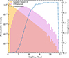 |
Fig. A.1. Sampled stellar mass function from Weibel et al. (2024, orange), together with the SFR-selected mass function (pink). The completeness trend, derived as the ratio of these two, is shown as dashed blue lines. |
Appendix B: Truncated skewed distribution
Here we describe the skewed normal distribution implemented in the Bayesian model described in Sect. 3.3. In particular, the fitted relation in the log-log space is
 (B.1)
(B.1)
with α = ms_slope and β = ms_norm, the intercept at log(M★/M⊙) = 10.5. We use the notation  to indicate a skewed normal distribution with zero mean and variance σeff2, where
 ![Mathematical equation: $ \sigma_{eff} = \sigma_{\mathrm{int}} \sqrt{ \left[ 1 - 2\delta^2/\pi \right]} $](/articles/aa/full_html/2026/03/aa57790-25/aa57790-25-eq76.gif) and
and  . The functional form of the intrinsic scatter is the same as in Eq. 3 and a_skew is the skewness parameter. Each skewed normal is truncated to mimic the selection effect resulting from flux-limited surveys, resulting in the selection-corrected probability p. We use the log-likelihood function as the objective function for MCMC parameter exploration, identifying the combinations of parameters (ms_slope, ms_norm, a, b, a_skew) that best describe the observed sample by maximizing likelihood.
We apply this model to the full SPHINX catalog at z = 4.64 after imposing a cut at SFR = 0.6M★/M⊙. We multiply our likelihood function ℒ by a uniform prior probability distribution, with each parameter restricted to the range: ms_slope = [0.2,1.8], ms_norm = [0.01,2.4], a = [ − 0.1, 0.3], b = [0.1, 1.3] and a_skew =[−5, 1]. We use MCMC sampling to explore the parameter space and determine the posterior distribution for each free parameter.
Figure B.1 shows the posterior distributions for the slope, normalization and σeff at two stellar masses. The slope and normalization are consistent with those found using truncated normal distributions (see Table 2). The skewness parameter, which enters σeff via the posterior distribution of a_skew, a and b, assumes the negative value a_skew = =  suggesting a tail toward lower SFRs as predicted from simulations (McClymont et al. 2025). We also apply this truncated skewed model to the THESAN-ZOOM data, recovering a_skew
  and estimates for the slope and normalization consistent with those of Table 2.
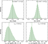 |
Fig. B.1. Posterior distributions for the slope, normalization and effective scatter of the SFMS from SPHINX simulation at z = 4.64. |
All Tables
All Figures
|
Fig. 1. F356W grism spectra for six Hα emitters in our sample. At the top of each panel, we report the stellar mass of the galaxy. The shaded region shows the uncertainty on the flux, and the 1.5″ × 1.5″ insets show false-color rest-frame optical RGB images constructed from NIRCam F115W/F200W/F356W. The green and brown lines highlight the Hαλ6564.6 and [N II] λλ6549.9, 6585.4 wavelengths, respectively. |
| In the text | |
|
Fig. 2. Projected separation between all pairs of galaxies in our sample with Δv < 1000 km s−1. The dashed vertical line at 0.8″, which corresponds to ∼5.5 kpc at z = 4.3, is our choice for the maximum angular separation among components belonging to the same system. |
| In the text | |
|
Fig. 3. Observed Hα fluxes as a function of redshift. We show the parent Hα sample (N = 512) in gray, and we highlight the robust sample in pink (N = 316, observed Hα flux > 10−18 erg s−1 cm−2 and μ ≤ 2.5). The red hexagons highlight the six confirmed broad-line Hα emitters (BLHα), with vFWHM > 1000 km/s, presented in Matthee et al. (2025). The hsistograms show the redshift and Hα flux distributions for the parent and robust samples. |
| In the text | |
|
Fig. 4. Probed parameter space in the SFR–M★ plane. The parameter space probed by ALT (pink) compared to that of the CONGRESS survey (green). The two surveys cover Hα emission in the redshift range z = 3.7 − 5.1. CONGRESS (Egami et al. 2023; Covelo-Paz et al. 2025) employs F356W grism in the GOODS-North field and captures galaxies with a median stellar masses higher than those from ALT, while ALT extends the parameter space approximately 2 orders of magnitude lower in stellar mass. |
| In the text | |
|
Fig. 5. Top: Model we used to describe the observed SFMS. The gray cloud represents all the HAEs in ALT, while the pink one is the observed sample after applying the selection criteria for robustness. Red points are the observed SFR, whose probability at fixed stellar mass is modeled using a truncated normal distribution that can be mass dependent. The normal distributions are centered in the SFR values predicted using the observed stellar masses and Eq. (2) whose parameters are explored within the MCMC sampling. Bottom: Toy model results. Mock observations generated sampling the stellar mass function from Weibel et al. (2024) with n_samples = 30 000. Gray dots show the entire sample, purple circles are galaxies with SFR > 0.7 M⊙/yr. The solid black line is the fit to the entire sample, while pink dashed and purple solid lines respectively show the fits with and without truncated normal distributions in the Bayesian model. The error bar in the bottom right is the 0.1 dex uncertainty on the SFR for each mock observation, corresponding to the average star formation rate uncertainty derived from observational data. |
| In the text | |
|
Fig. 6. Obscured star formation as a function of the stellar mass. The fraction of dust attenuated Hα emission, i.e., the ratio of the obscured and total Hα luminosity, as a function of stellar mass for the ALT sample. In gray is the parent Hα sample, while highlighted in pink is the robust one. Median values in each mass bin are shown as filled circles. Empty markers show obscured Hα fraction once we account for enhanced dust attenuation in high-mass galaxies (see Sect. 5.4). As a comparison, we show the fraction of obscured star formation for galaxies at 2 < z < 2.5 from Whitaker et al. (2017, blue), at 0.7 < z < 2 from Shivaei et al. (2024, green), and at z ∼ 4.5 ALPINE galaxies from Fudamoto et al. (2020, orange), with squares showing individual FIR continuum detections at 4 < z < 5 and triangles the 3σ upper limits for IR non detections. Filled squares show stacks in 2 mass bins at z ∼ 4.5. |
| In the text | |
|
Fig. 7. SFR–M★ relation at 3.7 < z < 5.1. In gray is the entire ALT Hα sample, while highlighted in pink is the robust subsample. Circles show the median value when binning in stellar mass (upper panel). We are > 90% mass complete for galaxies with log(M★/M⊙) > 8.5 (filled circles). For reference, we show the SFMS fits by Speagle et al. (2014, together with its 0.3 dex scatter) and Popesso et al. (2023) from a compilation of literature observations and the fit by Khusanova et al. (2021) from ALMA-ALPINE observations. Dotted lines mark extrapolations to these relations based on their lower limits on M★. Solid pink line and shaded region denote respectively the best-fit line and 1σ interval about the SFMS using the reference model that accounts for the selection function (see Sect. 3.3). |
| In the text | |
|
Fig. 8. Output of our reference model. Corner plot and posterior distributions (pink) of the four key parameters in our reference model: SFMS slope and normalization at log(M★/M⊙) = 10.5 (ms_slope, ms_norm) and the slope and normalization of the intrinsic scatter (a, b). The contours show the 1σ, 1.5σ, and 2σ confidence levels. We adopted truncated normal distributions to model the SFRs distribution in our Bayesian model (see Sect. 3.3). In purple we show the posterior distributions after running the Bayesian model on the robust sample imposing a Gaussian prior (mean = 1 and σ = 0.02) on ms_slope, referred to as “fixed ms_slope” in the legend. Above each panel we report medians with uncertainties (16th and 84th percentiles), those with asterisks refer to fixed ms_slope. The inset panels on the right show the intrinsic scatter distributions at two stellar masses, computed combining the posterior distributions for a and b with Eq. (2), and the σint evolution with stellar mass for the reference model and the model with a fixed ms_slope. |
| In the text | |
|
Fig. 9. Comparison with literature studies in the redshift range 4 < z < 5. The robust Hα sample used in this work and its binned values are in pink circles, blue and green triangles are mass binned observations from CONGRESS (Covelo-Paz et al. 2025) and, CEERS and JADES JWST-surveys (Clarke et al. 2024), respectively. Orange squares show observations from ALMA-ALPINE (Faisst et al. 2020), while the red square is the binned value for the ASPIRE survey which combines JWST and ALMA observations (Sun et al. 2025). To guide the eye, we show a linear relation with slope one (dashed black). |
| In the text | |
|
Fig. 10. Comparison between our inferences from observations and hydrodynamical simulations. Posterior distributions for the slope, normalization and intrinsic scatter of the SFMS. We compare the posteriors based on the ALT robust Hα sample (pink, hatched) explored in this work with those from dustyGadget (brown; Graziani et al. 2020; Di Cesare et al. 2023), EAGLE (blue; Schaye et al. 2015; Crain et al. 2015), IllustrisTNG-50 (orange; Pillepich et al. 2019; Nelson et al. 2019), SPHINX (green; Rosdahl et al. 2018, 2022; Katz et al. 2023) and THESAN-ZOOM (gray; McClymont et al. 2025) simulations. |
| In the text | |
|
Fig. 11. Effect of the new luminosity and EW-dependent SFR(Hα) calibrations. Comparison of the posterior distributions for the slope, normalization and intrinsic scatter of the observed SFMS, adopting diverse LHα–SFR conversions. In pink are those derived using the calibration from Theios et al. (2019) (ref.), in blue and yellow are the distributions using calibrations based on SPHINX simulations (Kramarenko et al. 2026). Specifically, in blue we show the posteriors derived from calibrations based on LHα of the galaxies, while in yellow those combining the information from LHα with that from the EWHα. |
| In the text | |
|
Fig. A.1. Sampled stellar mass function from Weibel et al. (2024, orange), together with the SFR-selected mass function (pink). The completeness trend, derived as the ratio of these two, is shown as dashed blue lines. |
| In the text | |
|
Fig. B.1. Posterior distributions for the slope, normalization and effective scatter of the SFMS from SPHINX simulation at z = 4.64. |
| In the text | |
Current usage metrics show cumulative count of Article Views (full-text article views including HTML views, PDF and ePub downloads, according to the available data) and Abstracts Views on Vision4Press platform.
Data correspond to usage on the plateform after 2015. The current usage metrics is available 48-96 hours after online publication and is updated daily on week days.
Initial download of the metrics may take a while.