| Issue |
A&A
Volume 707, March 2026
|
|
|---|---|---|
| Article Number | A281 | |
| Number of page(s) | 15 | |
| Section | Planets, planetary systems, and small bodies | |
| DOI | https://doi.org/10.1051/0004-6361/202557807 | |
| Published online | 17 March 2026 | |
Observing spatial and temporal variations in the atmospheric chemistry of rocky exoplanets: Prospects for mid-infrared spectroscopy
1
Center for Space and Habitability, University of Bern,
Gesellschaftsstrasse 6,
3012
Bern,
Switzerland
2
SETI Institute,
189 N. Bernado Ave,
Mountain View,
CA
94043,
USA
3
Blue Marble Space Institute of Science,
Seattle,
600 1st Avenue,
WA
98104,
USA
4
ETH Zurich, Institute for Particle Physics & Astrophysics,
Wolfgang-Pauli-Str. 27,
8093
Zurich,
Switzerland
5
National Center of Competence in Research PlanetS,
Gesellschaftsstrasse 6,
3012
Bern,
Switzerland
★ Corresponding author: This email address is being protected from spambots. You need JavaScript enabled to view it.
Received:
23
October
2025
Accepted:
19
December
2025
Abstract
Context. Future telescopes such as the Large Interferometer For Exoplanets (LIFE) will enable the unprecedented characterisation of the atmospheres of nearby rocky exoplanets, probing mid-infrared signatures of key molecules (e.g. CO2, H2O, O3, and CH4). Whilst 4D spatial and temporal variations of Earth as an exoplanet are below spectroscopic detection limits, such variability is strongly planet-specific.
Aims. We investigated LIFE’s ability to detect 4D spatial and temporal variability in the atmospheres of tidally locked exoplanets.
Methods. We created daily synthetic LIFE observations of Proxima Centauri b in a 1:1 and an eccentric 3:2 spin-orbit resonance (SOR), using LIFESIM on spectra from daily 3D climate-chemistry model (CCM) outputs of an aquaplanet with Earth-like composition. The spectra assume an inclination of 70◦.
Results. Hemispheric distributions of temperature, clouds, and chemical species determine spectral signatures and variability with orbital phase angle. Such variability dictates the extent to which parameters (e.g. radius, temperature, or chemical abundances) can be reliably inferred from snapshot spectra at arbitrary viewing geometries. In the 1:1 SOR, the MIR spectra vary significantly with viewing geometry and indirectly probe atmospheric circulation. Nightside temperature inversions generate O3, CO2, and H2O emission features, though these lie below LIFE’s detection threshold; instead, O3 features disappear at certain phase angles. In contrast, the 3:2 SOR yields a more homogeneous atmosphere with weaker phase variability but enhanced bolometric flux due to eccentric heating. Phase-resolved LIFE observations confidently distinguish between the SORs and capture seasonal O3 variability for golden targets such as Proxima Centauri b. In the case of abiotic O2 and O3 build-up, the O3 variability presents a potential false positive scenario.
Conclusions. Hence, LIFE can disentangle different spin-orbit states and resolve 4D atmospheric variability, enabling the daily characterisation of the 4D physical and chemical state of nearby terrestrial worlds. Importantly, this characterisation requires phase-resolved rather than snapshot spectra.
Key words: planets and satellites: atmospheres / planets and satellites: composition / planets and satellites: detection
© The Authors 2026
 Open Access article, published by EDP Sciences, under the terms of the Creative Commons Attribution License (https://creativecommons.org/licenses/by/4.0), which permits unrestricted use, distribution, and reproduction in any medium, provided the original work is properly cited.
This article is published in open access under the Subscribe to Open model. This email address is being protected from spambots. You need JavaScript enabled to view it. to support open access publication.
1 Introduction
Whilst the James Webb Space Telescope is starting to characterise the atmospheres of favourable rocky exoplanets, the next-generation observatories are being developed and designed to further advance the quest for atmospheric biosignatures. Amongst them are the Extremely Large Telescope, the Habitable Worlds Observatory (HWO), and the Large Interferometer For Exoplanets (LIFE). LIFE is a space-based nulling interferometer that will observe at mid-infrared (MIR) wavelengths, and will provide a unique spectroscopic window into the direct thermal emission of rocky exoplanets (Quanz et al. 2022; Glauser et al. 2024). The thermal emission spectra will probe the atmospheric structure, chemical signatures, and their potential spatial and temporal variations. Therefore, any robust interpretation of the spectra will require a thorough understanding of the stellar and planetary environmental context, especially when distinguishing potential biosignatures from false positive scenarios (e.g. Catling et al. 2018; Meadows et al. 2018). Here, we evaluate synthetic MIR spectra based on a comprehensive climate-chemistry model (CCM) to investigate this environmental context and determine LIFE’s ability to characterise varying chemical signatures.
Before any such atmospheric characterisation, LIFE is designed to start with a search phase resulting in a detection yield of several hundred exoplanets (Quanz et al. 2022; Dannert et al. 2022; Kammerer et al. 2022). The most promising planets will be targeted for atmospheric characterisation, including planets in M-star habitable zones (typically at ∼5 pc) and FGK-star systems (typically at ∼10 pc; Dannert et al. 2022; Kammerer et al. 2022; Angerhausen et al. 2024). LIFE can characterise an Earth-twin with detected features of ozone (O3), methane (CH4), carbon dioxide (CO2), and water vapour (H2O; Konrad et al. 2022), and can distinguish between different eras of Earth’s geological and atmospheric evolution (Alei et al. 2022). The atmosphere of a Venus-like exoplanet can be characterised above the cloud deck by LIFE, although 1D retrievals struggle to retrieve cloud properties (Konrad et al. 2023). More exotic biosignatures, including nitrous oxide (N2O), methylated halogens, and phosphine, are also detectable by LIFE (Angerhausen et al. 2023, 2024) at plausible biological fluxes and observation times. There are strong synergies between LIFE and HWO, both in terms of planet detection (Carrión-González et al. 2023) and robustly characterising the atmospheric structure and chemical signatures (Alei et al. 2024), although LIFE has the advantage that it can observe exoplanets on close-in orbits around M stars. To date, the majority of studies exploring LIFE’s characterisation capabilities have employed 1D models of atmospheric physics and chemistry.
However, Earth’s atmosphere demonstrates substantial variations in its physical and chemical characteristics, in three spatial and one temporal dimension, which in turn lead to 4D variations affecting Earth’s (MIR) spectrum (e.g. Des Marais et al. 2002; Tinetti et al. 2006a,b; Hearty et al. 2009; Gómez-Leal et al. 2012). Since atmospheric seasonality on Earth is biologically modulated, temporal (or seasonal) variations have been proposed as a potential biosignature (Olson et al. 2018). Importantly, observed emission spectra will always be hemispheric averages with unresolved spatial and temporal variations, presenting possible degeneracies in interpretation. Mettler et al. (2023) construct disk-integrated MIR thermal emission spectra of Earth to study the variations of Earth’s thermal emission spectrum with viewing geometry, phase angle, and seasons, using remote sensing data of four viewing geometries with high temporal, spatial, and spectral coverage. Moreover, they quantify the atmospheric seasonality of potential biosignatures such as O3, CH4, N2O, and CO2. Mettler et al. (2023) demonstrate that Earth’s disk-integrated thermal emission spectrum varies significantly with seasons and viewing geometry. The combination of disk-integrated data and annual variability produces degeneracy in the spectrum. To break this degeneracy for Earth, we need more than a single-epoch or snapshot spectrum and to cover (part of) the phase angle variations with multiple spectra (Mettler et al. 2023). The atmospheric seasonality in biosignature abundances on Earth generally remains below 5% (except for CO2 at 8.6 and 15.8% over the North and South Poles, respectively).
In a follow-up paper, Mettler et al. (2024) comprehensively assess the potential to detect these biosignatures and their variations as well as the impact of the viewing geometry and seasonality for Earth from 10 pc. They create synthetic 30-day LIFE observations of Earth’s MIR spectrum using LIFESIM (Dannert et al. 2022) and compare the subsequent atmospheric retrieval results to the ground truths. LIFE can easily detect a habitable planet (e.g. by constraining temperature and albedo) with static detections of CO2, H2O, O3, and CH4, confirming earlier findings (Konrad et al. 2022; Alei et al. 2022). In the case of a well-constrained planet radius, seasonal variations in the surface temperature, equilibrium temperature, and bond albedo are detectable (Mettler et al. 2024). However, the retrieved surface pressure, pressure-temperature profile, and trace abundances have biases, mainly due to assumed constant abundance profiles and the lack of a patchy cloud treatment in the retrieval frameworks, which are both addressed in Konrad et al. (2024). Earth’s spatial and temporal variations in chemical abundances are too small to be detected (Mettler et al. 2024), thus hindering biosignature detection through seasonality for exoplanets similar to Earth.
However, many of the currently known rocky exoplanets exhibit orbital configurations that are distinct from Earth’s. Since (rocky) exoplanets are most easily detected orbiting close-in to relatively cool stars, the timescales of tidal locking are much shorter than planetary lifetimes, and they end up in spin-orbit resonances (SORs) (Goldreich & Peale 1966; Barnes 2017; Pierrehumbert & Hammond 2019). Tidal locking timescales are particularly short for exoplanets around M and K stars and remain shorter than 1 Gyr for K6 stars (Barnes 2017). The outcomes of tidal locking include various ratios of SORs (Goldreich & Peale 1966; Dobrovolskis 2007; Renaud et al. 2021), depending on eccentricity (amongst others). Furthermore, close-in rocky exoplanets may have passed through dynamical cascades of SORs during their evolutionary history (Renaud et al. 2021), including higher-order resonances. However, the effects for the climatic and dynamical state of a planetary atmosphere are most extreme for the 1:1 and 3:2 SORs, whilst higher-order resonances are more subtle variations of the latter (e.g. Dobrovolskis 2007; Colose et al. 2021). Proxima Centauri b (Anglada-Escudé et al. 2016) is the nearest exoplanet and, located in the habitable zone (HZ) of its M5.5V host star, most likely orbits in such a SOR. Furthermore, it is non-transiting, making it ideally suitable for MIR thermal emission spectroscopy. The small distance to Proxima Centauri b (1.032 pc) implies that LIFE can obtain high-quality spectra in observation times of the order of days, making it a golden target for the mission with potential characterisation of spatial and temporal variations in its atmosphere (Angerhausen et al. 2024).
A substantial body of theoretical work has hypothesised on the extent of these spatial and temporal variations for Proxima Centauri b and similar exoplanets in SORs, using general circulation models. In the case of a 1:1 SOR, substantial dayside– nightside or longitudinal variations are commonly predicted in meteorological quantities such as irradiation, temperature, and cloud cover (e.g. Turbet et al. 2016; Boutle et al. 2017; Del Genio et al. 2019; Sergeev et al. 2020). On the other hand, an eccentric 3:2 SOR exhibits a 180◦ shift in the substellar point for every orbit around the star, providing a day–night cycle and latitudinal variations in meteorological quantities (Turbet et al. 2016; Boutle et al. 2017; Del Genio et al. 2019; Braam et al. 2025). The 3:2 SOR also generally warms the planet, associated with a weaker cloud feedback and eccentric orbit (Colose et al. 2021). The interplay between stellar irradiation, atmospheric dynamics, thermodynamics, and (photo)chemistry determine the spatial and temporal distribution of chemical species for either SOR. Studies using 4D CCMs consistently show substantial dayside–nightside spatial asymmetries in chemical abundances for a 1:1 SOR (e.g. Chen et al. 2018; Yates et al. 2020; Braam et al. 2023; Cooke et al. 2024), whereas meridional gradients are expected for a 3:2 SOR (Braam et al. 2025). Additionally, temporal variations are caused by a planet’s orbital evolution (e.g. Way & Georgakarakos 2017; Chen et al. 2023; Braam et al. 2025), internal atmospheric variability (Hochman et al. 2022; Cohen et al. 2023; Luo et al. 2023), or external events such as flares (e.g. Chen et al. 2021; Ridgway et al. 2023; Chen et al. 2025). Many of the spatial and temporal variations are more pronounced compared to those on Earth.
The spatial and temporal variations, in turn, affect spectroscopic observations of the atmospheres in transmission (Chen et al. 2021; Cohen et al. 2023), reflection (Cooke et al. 2023b), and emission spectra (Braam et al. 2025). Variations with seasons or viewing angles depend on the star-planet system, with magnitudes of spectral variations in thermal emission spectra for exoplanets in 1:1 SOR exceeding those of a 3:2 SOR or Earth (Mettler et al. 2023; Braam et al. 2025). Many false positive scenarios have been reported for static biosignatures, such as the abiotic build-up of O2 and O3 (e.g. Hu et al. 2012; Domagal-Goldman et al. 2014; Tian et al. 2014; Harman et al. 2015). Another robust indicator of biological activity is seasonality in molecular abundances of species such as O3 (Olson et al. 2018; Schwieterman et al. 2018). However, if an abiotic pathway to their production exists, abiotic spatial and temporal variations due to orbital geometry or internal variability present a potential false positive alternative to seasonal variations in biosignatures that need to be ruled out based on environmental context (Fujii et al. 2018; Meadows et al. 2018).
For this paper we investigated LIFE’s ability to detect 4D spatial and temporal variability in the atmospheres of tidally locked exoplanets, based on comprehensive 4D CCM simulations. Our aim was to distinguish between different SORs and to quantify the spectral variations in O3 due to the planetary and orbital context. In Sect. 2, we describe the creation of time-resolved synthetic LIFE spectra based on the 3D spatial distributions from the CCM simulations. In Sect. 3 we present the observed spatial distributions, the synthetic LIFE observations, circulation-induced spectral variations, and tie everything together in an analysis of temporally varying O3 features. We put our results into context and compare them to Earth in Sect. 4, before concluding our study in Sect. 5.
2 Methods
2.1 4D atmospheric chemistry
The data underlying this study were produced using a state-of-the-art CCM – the Met Office Unified Model in its coupled version to the UK Chemistry Aerosols framework (UM-UKCA) – and based on the simulations that were analysed in Braam et al. (2025). The modelling framework was initially developed to model Earth’s atmosphere and the Earth System (see e.g. Walters et al. 2019; Archibald et al. 2020). Here, we briefly discuss the adaptation to terrestrial exoplanets, focusing on the key components of the simulations. For extensive detail on the exo-planet adaptation, we refer to Mayne et al. (2014), Boutle et al. (2017), Yates et al. (2020), Braam et al. (2022), and Braam et al. (2025).
We used UM-UKCA to simulate a 1.1 R⊕ aquaplanet with an Earth-like atmosphere in the orbital configuration of Proxima Centauri b (Anglada-Escudé et al. 2016). The flat and homogeneous surface is a 2.4 m slab ocean layer without heat transport and has a resolution of 2 by 2.5◦ in latitude and longitude (Boutle et al. 2017). The Earth-like atmosphere provides a 1 bar surface pressure, and extends up to 85 km in altitude (or a pressure of 9 × 10⁻⁵ or 1.3 × 10⁻⁴ bar, see Braam et al. 2025). We initialised the atmospheric composition with abundances of N2, O2, and CO2 based on the atmosphere of pre-industrial Earth, and water vapour (or H2O (g)) forms thermodynamically from the surface/atmosphere balance. The radiative transfer scheme is the Suite of Community Radiative Transfer codes based on Edwards and Slingo (SOCRATES, see Edwards & Slingo 1996) which interactively calculates heating rates and drives the thermal and dynamical evolution of the atmosphere. The dependence of incoming radiation on the orbital configuration is described in Appendix A of Braam et al. (2025).
The orbital evolution also determines the photolysis rates of chemical species in the atmosphere, which are calculated in UM-UKCA following Telford et al. (2013) and the adaptation to exoplanets by Yates et al. (2020) and Braam et al. (2022). These photolysis rates are the ultimate driver of the (photo)chemistry in the model. The chemistry describes the Chapman mechanism of O3 formation, and the hydrogen oxide (HOx) and nitrogen oxide (NOx) catalytic cycles and is a reduced version of the Stratospheric-Tropospheric scheme presented by Archibald et al. (2020).
Following previous studies (Boutle et al. 2017; Turbet et al. 2016; Del Genio et al. 2019; Braam et al. 2025), we configured Proxima Centauri b in a 1:1 and 3:2 SOR, including an eccentricity of 0.3 for the latter (see e.g. Goldreich & Peale 1966; Dobrovolskis 2007). For the 1:1 SOR, the star–planet separation is fixed at 0.0485 AU, whereas it varies between 0.03395–0.063 AU for the 3:2 SOR. Furthermore, the rotation rate (or spin) of the 3:2 SOR is increased to 9.7517 × 10⁻⁶ (from 6.501 × 10⁻⁶ for the 1:1 SOR) to cover 1.5π rad of planetary rotation in one orbital period of 11.186 days. After spinning up the simulations to a steady state (7400 days for the 1:1 SOR and 17 000 days for the 3:2 SOR), we used the first orbit for the 1:1 SOR (12 days of daily output) and the first two orbits for the 3:2 SOR (24 days of daily output). Taking two orbits for the 3:2 SOR covers a full daytime-nighttime cycle for all locations on the planet (see Braam et al. 2025, for details). To determine the orbital phase angle of the planet, we followed the implementation of orbital astronomy in SOCRATES and the UM (Edwards & Slingo 1996; Manners et al. 2021) and calculated the mean and true anomaly as described in Smart (1944). The true anomaly ν(t) represents the angle between the direction of periastron from the barycentre and the position of a planet at the current time t in days. The mean anomaly M(t) is the fictitious angle from periastron for a planet on a circular orbit at the same time t, assuming the same semi-major axis as for the true elliptical orbit and is given by
 (1)
(1)
with tp the time when the planet is at periastron, and P the length of a year or orbital period (both in days). For a Keplerian orbit of eccentricity e, M(t) can be used to calculate the true anomaly ν(t), using the third-order approximation of a series expansion known as the equation of the centre (Smart 1944):
 (2)
(2)
For a circular orbit of e=0, M(t) and ν(t) are equal. Since we defined the longitude of perihelion in the simulations at 102.94◦ or 1.796601474 rad, the orbital phase angle θ(t) as a function of time is found by adding the longitude of perihelion to ν(t):
 (3)
(3)
The values of θ(t) and ν(t) for both the 1:1 and 3:2 SOR can be found in Table 1.
The hour angle for the 3:2 SOR (relative to hour angle 0 at perihelion) is given by
 (4)
(4)
where tD represents the length of day, which is equal to two orbital periods for a 3:2 SOR (and infinite for a 1:1 SOR). The equation of time is used to correct for the discrepancy between the mean and apparent solar (stellar) time when simulating an eccentric orbit and is added as a correction to the hour angle. For the simulations and orbital calculations, we used the equation of time following Mueller (1995) and Manners et al. (2021). Correcting for the clockwise rotation, 2π − HA then gives λSP(t), the substellar longitude as a function of time. For the 3:2 SOR, λSP(t) is given in Table 1; for the 1:1 SOR, the substellar point is always at 0◦ latitude and longitude.
True anomaly ν(t) and orbital phase angle θ(t) for Proxima Centauri b in a 1:1 and 3:2 SOR.
2.2 PSG spectra
The Planetary Spectrum Generator (PSG), developed by NASA, is a versatile radiative transfer model suite capable of synthesising planetary spectra across a wide range of wavelengths (Villanueva et al. 2018, 2022). For our study, we utilised the Global Emission Spectra (GlobES) application within PSG to generate emission spectra of exoplanets based on the output of 3D climate and chemistry simulations (Fauchez et al. 2025). GlobES has been used to produce spectra of TRAPPIST-1 e as part of the THAI papers (Fauchez et al. 2022), Earth as an exo-planet (Kofman et al. 2024), and Proxima Centauri b (Braam et al. 2025).
GlobES creates emission spectra based on 3D distributions of gaseous molecules, including H2O, O3, NO, and NO2, as well as ice and water clouds. We also incorporated iso-abundances of N2, CO2, and O2, along with collision-induced absorption (CIA) caused by O2-O2, O2–N2, N2–N2, and H2O–H2O pairs. The multiple scattering effects of aerosols, specifically ice and water clouds, and Rayleigh scattering are modelled using the PSGDORT module (Villanueva et al. 2022; Kofman et al. 2024) and wavelength-dependent extinction coefficients and scattering albedo are calculated using Mie theory. Surface reflection is Lambertian. Full radiative transfer calculations are performed for these 3D distributions, taking emission angles into account. A detailed description of the GlobES tool can be found in Kofman et al. (2024) and Fauchez et al. (2025).
Our orbital geometry configuration incorporates the standard stellar and orbital parameters for the Proxima Centauri system, assuming an inclination of 70◦ following Braam et al. (2025). For the planet in 1:1 SOR, the substellar point is fixed at 0 degrees longitude, with the orbital phase angle varying as shown in Table 1. For the 3:2 SOR, the substellar longitude and orbital phase angle change over time, following the values in Table 1. PSG accounts for the planet’s eccentricity, resulting in a variable star–planet separation ranging from 0.03395 AU at periastron to 0.06305 AU at apoastron. Standardised configuration files for both SORs and code to convert the CCM data into binary format for the PSG configuration files are available online1. For each combination of orbital phase angle, substellar longitude, and climate-chemistry state, PSG calculates the spectral radiance at the top of the atmosphere in units of W sr−1 m−2 µm−1.
Overview of simulation parameters used in LIFESIM, following Quanz et al. (2022) or Angerhausen et al. (2023).
2.3 LIFESIM
Following the generation of emission spectra as described in Sects. 2.1 and 2.2, we employed the LIFESIM software to calculate (feature) detectability of the emission spectra, following methodologies from Angerhausen et al. (2023) and Angerhausen et al. (2024). Key simulation parameters are summarised in Table 2. The reference architecture enables atmospheric characterisation through MIR spectroscopy while balancing sensitivity and technical feasibility (Dannert et al. 2022; Kammerer et al. 2022; Angerhausen et al. 2023). We assumed 24 hours of observation time, matching the temporal resolution of the CCM output and following earlier assessments of LIFE observations for Proxima Centauri b (Angerhausen et al. 2024).
3 Results
We start this section by discussing the observed spatial distributions for different phase angles and their effects on the spectral radiance. We then present simulated LIFE observations and the implications for the observing strategy. The final two subsections outline the prospects for circulation-induced spectral features and seasonally varying biosignatures.
3.1 Observed spatial distributions
Figure 1 shows how the observed hemispheric distributions of four key quantities change with θ(t), based on our simulations of Proxima Centauri b in a 1:1 and 3:2 SOR. Shown are: surface temperature Ts in K, the vertically integrated water vapour column density σH2O in molecules m−2, the vertically integrated total cloud water path (CWP) in kg m−2, and the vertically integrated O3 column density σO3 in molecules m−2. We include the distributions for four distinct phase angles to demonstrate the extrema in these quantities from an observational perspective. This work aims to connect the predicted 4D spatial and temporal distributions of the Proxima Centauri b simulations to potential observability with LIFE. Therefore, here we only discuss the key characteristics of the observed hemispheric distributions. For more comprehensive descriptions of the physical and (photo)chemical processes underlying the hemispheric distribution, we refer to Boutle et al. (2017) and Braam et al. (2025).
For each θ(t), we calculate the hemispheric mean of the four quantities over the hemisphere visible to a distant observer at that time (see Fig. 2 or Tables A.1 and A.2). Additionally, we calculate the hemispheric mean volume mixing ratio of O3 (χO3,strat) in the stratosphere, represented by the vertical mean over layers between 100–0.1 hPa. For the 1:1 SOR, the effects of the synchronous orbit are clearly visible. At θ=1◦, the observed hemisphere mainly covers the dayside (top panel of Fig. 1), with maxima in  ,
,  molecules m−2,
  , and minima in
  molecules m−2 (Fig. 2). Close to first quadrature, at θ=98◦, Fig. 1 shows that the observed hemisphere is comprised of both the dayside and nightside hemispheres, with lower
  ,
,  molecules m−2, and
  , as well as higher
  molecules m−2. This trend is continued until conjunction, where we mainly observe the nightside hemisphere as illustrated in Fig. 1 for θ = 200◦. Now, the averages on the observed hemisphere reach minima in
  ,
,  molecules m−2, and
  and maxima in
  molecules m−2. Lastly, the third quadrature shows part of the dayside and part of the nightside hemisphere again, similarly to the first quadrature and reflected in the observed hemispheric averages in Fig. 2 and Table A.1. Figure 2 shows how χO3,strat only varies by up to 1%. These small variations agree with a long chemical lifetime for stratospheric O3 (10–1000 years) as compared to an orbital period (Braam et al. 2023).
For the 3:2 SOR, the bottom panel of Fig. 1 illustrates the effect of a non-synchronous tidally locked orbit. Due to the enhanced planetary spin velocity and thus the absence of a permanent dayside hemisphere, the distributions of  ,
,  ,
,  , and
, and  are more homogeneous (compared to the 1:1 SOR). This enhanced homogeneity is reflected in the hemispheric averages for the observed hemispheres in Fig. 2. We find maxima in
  ,
,  molecules m−2, and
  and minima in
  molecules m−2 for θ∼280◦. In this case, we observe the side of the planet that was previously subjected to the strongest radiation during the daytime at periastron passage. On the other hand, we find minima in
  ,
,  molecules m−2, and
  for θ∼0◦ (observing the side that was illuminated at apoastron) and maxima in
  molecules m−2 slightly earlier in the orbit for θ = 295◦. Stratospheric variations are enhanced compared to the 1:1 SOR, with χO3,strat variations up to 3.6%.
Figure 3a shows the simulated emission spectra for Proxima Centauri b in a 1:1 SOR, as modelled by the GlobES tool of PSG (see Sect. 2.2). For the 1:1 SOR, we include daily spectra to show the dependence on θ(t). The maximum continuum emission (e.g. as probed between 10–12.5 µm) is received for θ = 1◦, in line with Fig. 1 where we observe most of the dayside hemisphere. The planet then goes through phase angles for which we observe a combination of the dayside and nightside hemispheres, leading to lower emission, until the point of minimum emission, when mainly the nightside hemisphere is observed (e.g. at θ = 162, 168 or 200◦). Relative to the blackbody curves, the continuum ranges from roughly midway between the 225 and 250 K blackbodies down to the 200 K curve. The CO2 feature between 14–16 µm originates from the relatively cool stratosphere and therefore even approaches the 185 K blackbody curve.
The absorption due to the main O3 feature (around 9.6 µm) is deepest when most of the dayside is in view. As we transition to observing the nightside hemisphere, O3 absorption is still present but less prominent (e.g. at θ = 162, 168, or 200◦). Additionally, the outer regions become emission features, likely due to the formation of a tropospheric inversion layer (e.g. Guzewich et al. 2020). The varying depth and behaviour of the O3 feature suggest that a statistically significant O3 detection might be dependent on the observed phase angle. Similarly, the 4.8 µm O3 feature is deepest when the dayside is most into view. However, the generally shallower feature at this wavelength completely disappears for all but the brightest phase angles. The features due to CIA by O2-O2 and O2–N2 pairs (between 5.2–7.4 µm) are mainly overshadowed by the stronger H2O features in the same region. Nevertheless, the narrow peak in the middle (centred at 6.4 µm) may be identified as an O2 signature as long as the phase angle dependence of the H2O features is known.
The H2O features (5–8 and 16.5–18.5 µm) vary as expected: with the hottest and thus wettest observed hemispheres (θ = 1, 33, 66, 329◦) resulting in the strongest emission. Transitions between absorption and emission features are seen at 7.9 (H2O), 12.6 (CO2), and 18.3 µm (H2O). When we mainly observe the dayside hemisphere, we tend to see absorption as compared to surrounding wavelengths, which changes to emission when we mainly observe the nightside. These features originate in the troposphere and are thus affected by the nightside tropospheric temperature inversion: they originate at higher temperatures than the surrounding features (e.g. Guzewich et al. 2020).
For the 3:2 SOR in Fig. 3b, the more homogeneous atmosphere substantially reduces the phase angle variations. Furthermore, the higher spin rate and eccentric orbit affect the appearance of maxima and minima in the spectral radiance. As shown in Table A.2, observed hemispheric temperature maxima are found at phase angles close to apoastron (e.g. 250–290◦), when the hemisphere that was subjected to periastron irradiation comes into view. However,  is also twice as high on the observed hemispheres around apoastron compared to low phase angles (e.g. 12 and 48◦), offsetting the relatively small temperature changes. The maximum continuum emission in Fig. 3b comes from θ = 48◦, due to this combined effect of planetary temperature and cloud thickness. The continuum emission is closest to the 250 K blackbody curve, regardless of phase angle, due to the warmer atmosphere of a 3:2 SOR compared to a 1:1 SOR. The 9.6 µm O3 and 14–16 µm CO2 features originate in the cooler stratosphere, thus approaching the 200 K and 185 K curves, respectively. Phase angle variations in individual chemical signatures (e.g. O3 or H2O) are minimal in this case, thus reducing the potential ambiguity in detecting these species.
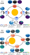 |
Fig. 1 Observed hemispheric distributions as a function of θ(t) for the 1:1 SOR (top) and the 3:2 SOR with an eccentricity of 0.3 (bottom): surface temperature (blue-red), vertically integrated water vapour or H2O (g) column density (white–blue), vertically integrated total cloud path (white-grey), and vertically integrated O3 column density (dark blue– yellow). The longitude of perihelion of the 3:2 SOR is at 102.94◦. For both SORs, we use four extreme cases of θ(t) (see Table 1). The distributions vary spatially and temporally, illustrating the orbital evolution of climate and chemistry, as well as the effects of viewing geometry. |
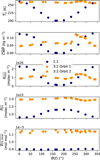 |
Fig. 2 Phase angle evolution of the hemispheric means across the observed hemisphere of Proxima Centauri b in 1:1 SOR (navy) and 3:2 SOR (orange), for the quantities shown in Fig. 1 and |

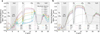 |
Fig. 3 Simulated spectral radiance at the top of the atmosphere for Proxima Centauri b in (a) 1:1 SOR and (b) 3:2 SOR, for θ(t) as shown in Table 1. The spectra were created using PSG and the GlobES tool (see Sect. 2.2 for details). We also include blackbody curves at different temperatures for comparison and grey rectangles for important molecular and CIA features. For panel (b), the solid and dashed lines represent the first and second orbits around the host star, respectively, and together correspond to the length of a full day for the 3:2 SOR. |
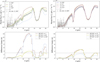 |
Fig. 4 Example simulated LIFE observation for the 1:1 resonance case (left) and 3:2 resonance case (right) assuming an integration time of 24 hours. The grey area represents the 1σ sensitivity; the dark grey error bars show an individual simulated observation. Lower panel: Statistical significance of the detected differences between different phases. |
3.2 LIFE observations and consequences for observation strategy
Proxima Centauri b has previously been identified as a golden target for LIFE, due to its relative proximity to the Solar System (Angerhausen et al. 2024), potentially allowing detailed and time-resolved observations of the planet. Angerhausen et al. (2024) test the observability of a ‘static’ Earth-like exoplanet with varying biogenic fluxes, and find that detailed observations are already possible with just 24 hours of observational time with LIFE. Here, we expand upon their results by employing LIFESIM (Dannert et al. 2022) to create synthetic time-resolved observations with LIFE based on the CCM simulations in Sect. 3.1. We also assume 24 hours of observational time with LIFE, in agreement with the temporal resolution of CCM output. Figure 4 shows the predicted LIFE observations in a phase comparison for Proxima Centauri b, comparing LIFE observations at distinct phase angles for the 1:1 SOR (left) and the 3:2 SOR (right).
Focusing on the observations for the 1:1 SOR at θ = 265◦, we first see that LIFE can conduct a detailed characterisation of the spectrum for a specific phase angle in one Earth day. LIFE clearly captures the O3 and CO2 features and is also sensitive to the extent of the H2O features between 16.5–18.5 µm. Second, LIFE is highly sensitive to the spectral changes with θ for the 1:1 SOR. The statistical significances of observed differences between phase angles are shown in the bottom panels of Fig. 4. For the 1:1 SOR, the statistical differences reach 12 σ in the continuum level and ∼8σ for the H2O features. Moreover, compared to θ = 1◦ or 98◦, the observed differences around the 9.6 µm O3 feature are significant near the 3σ level. Clearly, daily LIFE observations will provide detailed information on changes in the chemical state (O3 and H2O abundances and distributions) and physical state (temperature, clouds, and H2O distributions) of the planetary atmosphere. Hence, the high spectral and temporal resolution with LIFE observations of Proxima Centauri b allow us to probe the dynamic atmosphere on a daily basis.
The comparison with the 3:2 SOR in the top left panels of Fig. 4 confirms the eccentricity-induced global temperature enhancement for the 3:2 resonance, with generally higher continuum fluxes than the 1:1 SOR. Even though the atmosphere of the 3:2 SOR is more homogeneous (see Sect. 3.1), LIFE observations still vary with θ at up to ∼5σ significance, providing a potential probe to the extremes of the dynamic atmosphere given LIFE’s spectral and temporal resolution. Nevertheless, the emission differences with θ are considerably smaller for the 3:2 SOR, providing a clear distinction from a planet in a 1:1 SOR. The low nightside continuum emission for the 1:1 (see the θ = 168◦) is key to making this distinction. The homogeneous distribution of photochemical species such as O3 for a 3:2 SOR makes the spectral variations even smaller at the relevant absorption wavelengths (see the 9.6 µm features). Therefore, a phase curve centred at the O3 feature (or features of other prominent photochemical species) is an excellent probe of SORs.
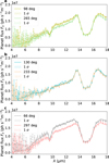 |
Fig. 5 Pairs of simulated LIFE spectra for the 1:1 SOR at similar distances from phase angles of 90 and 270◦, illustrating the effects of the atmospheric circulation. Panel a shows spectra for phase angles 98 and 265◦, panel b for 130 and 233◦, and panel c for 66 and 297◦. |
3.3 Atmospheric circulation mechanisms
Beyond the orbital configuration, the spatial distributions of temperature, clouds, and chemical species are strongly affected by the atmospheric dynamics on a planet. The 1:1 versus 3:2 SOR comparison in Fig. 1 illustrates this most evidently in the O3 column density. Despite being photochemically produced, O3 accumulates on the nightside of the 1:1 SOR and at high latitudes for the 3:2 SOR due to their respective circulation regimes (Braam et al. 2025). The spectral variations in simulated LIFE observations for the 3:2 SOR are too small to provide us with clues to the specific circulation regime, especially since chemical abundances vary with planetary latitude. The longitudinal variations for a 1:1 SOR leave more promising phase angle variations in the LIFE observations relating to the circulation regime.
For exoplanets in 1:1 SOR, the specific regime of atmospheric circulation is predicted to depend on the orbital period (e.g. Carone et al. 2015; Noda et al. 2017; Haqq-Misra et al. 2018) as well as model parametrisations (Sergeev et al. 2022b). The different circulation regimes for a 1:1 SOR will leave their marks in spatial distributions of temperature, clouds, water vapour and chemical abundances (e.g. Chen et al. 2019; Sergeev et al. 2022a; Braam et al. 2023). Proxima Centauri b simulations commonly exhibit an eastward equatorial jet in the troposphere. In Fig. 1 we see how the circulation regime manifests itself in higher  for a phase angle of 265◦ as compared to 98◦, as the eastward advection of the substellar cloud deck comes into view. The same mechanism might apply to two other pairs of phase angles: 233◦ versus 130◦ and 297◦ versus 66◦, although these contaminations from dayside-nightside differences are bigger due to a larger angular distance from 90◦ and 270◦.
We compare these phase angle pairs in the three panels of Fig. 5. The planet fluxes observed by LIFE are enhanced for a phase angle of 98◦ compared to 265◦ (Fig. 5a). Hence, despite the slightly lower  (0.6%, see Table A.1), the 3% lower
  allows planet flux to originate from deeper (and warmer) atmospheric layers. The flux differences are markedly weaker when comparing phase angles 130◦ and 233◦ (Fig. 5b). For these phase angles, LIFE mainly observes the nightside hemisphere with its horizontal asymmetries due to the Rossby gyres and vertical temperature inversions. Moreover, the actual values for
  are five times lower than phase angles 98◦ and 265◦, presenting too little cloud cover to be sensitive to the circulation mechanism. For phase angles 66◦ and 297◦ and Fig. 5c), LIFE again observes more planet flux for the smaller phase angle, which presents the lower
  (0.3%) and
  (5%). Moreover,
  is at similar levels to phase angles 98◦ and 265◦, giving enough cloud cover to provide sensitivity to the circulation mechanism. Hence, deliberate phase-resolved emission spectroscopy with LIFE can be used to confirm the predicted circulation mechanisms through the advection of the substellar cloud deck.
3.4 Temporally varying biosignatures
In Sects. 3.1 and 3.2, we identified different temporal variations due to the stellar and planetary environment and, in our work, in particular due to distinct SORs. Evidently, temporal variations in emission spectra arise due to 1) seasonality on a planet, driven by obliquity or eccentricity, and 2) orbital phase angle and viewing geometry in the case of spatial asymmetries in the planetary atmosphere. Since seasonality has previously been proposed as a biosignature, a thorough understanding of the robustness of seasonality as a biosignature is essential – particularly in the context of abiotic O2 and O3 build-up on exoplanets around M-dwarfs (e.g. Hu et al. 2012; Domagal-Goldman et al. 2014; Tian et al. 2014; Harman et al. 2015). Mettler et al. (2023) use time-series of remote sensing data of Earth’s atmosphere to show how Earth’s MIR spectrum varies with time, viewing geometry, and phase angle, focusing on absorption features of O3, CH4, CO2, and N2O. In our simulations, CO2 is fixed and CH4 absent, whereas abiotically produced N2O (lightning, photochemistry) is not abundant enough to be detectable (Braam et al. 2022). The 9.6 µm O3 feature, however, shows substantial variations (see Figs. 3 and 4). Hence, we can investigate the most physically and chemically self-consistent time series of O3 variations for the two SORs considered, given our model assumptions.
We follow the approach by Mettler et al. (2023) and calculate the equivalent width as a measure of the strength of an absorption or emission feature,
 (5)
(5)
where  is the radiance in our region of interest (in this case, the O3 feature at 9.6 µm, using outer bounds of 9.15–10.15 µm) and IC the continuum radiance in this same region, based on a fit to the wavelength regions surrounding the 9.6 µm O3 feature, specifically between 8–9.15 µm and 10.15–12.2 µm. We fit the continuum regions with a quadratic polynomial and normalise the radiance in the O3 band with the fitted continuum radiance, as in Eq. (5). Figure 6 demonstrates how this procedure allows us to isolate the O3 features, for both SORs. We note that our O3 bands are wider than the 0.7 µm band used by Mettler et al. (2023), motivated by the broad features originating from the nightside phase angles of the 1:1 SOR. Since these features emerge in the troposphere, they are likely subject to pressure broadening. The continuum fit slightly overestimates the lower wavelength continuum level for the 3:2 SOR in Fig. 6b, giving a normalised radiance below unity. However, it does not affect variations in Wλ since the normalised radiance is constant between 9.15–9.3 µm. The homogeneous atmosphere of the 3:2 SOR produces a fairly constant normalised radiance (Fig. 6b). On the other hand, the normalised radiance in the O3 band varies considerably for the 1:1 SOR. Notably, the 1:1 SOR shows the transitions between absorption and emission, with a normalised radiance smaller and greater than unity, respectively. The nightside phase angles (168 and 200◦) again correspond to O3 emission features that are due to the nightside temperature inversion (see Sect. 3.1).
The distinction between both SORs becomes even more apparent when considering the temporal variations of Wλ in Fig. 7. The phase angle variations represent the temporal evolution, and colours for each SOR match across Figs. 3–8 to identify the dependence on θ. For the 1:1 SOR (Fig. 7a), observations of the O3 band are mainly affected by the θ dependence, as the actual temporal variations of the spatial distribution are modest. For most of the orbit, the dayside hemisphere dominates the O3 feature, resulting in Wλ reaching up to 200 nm. A transition happens for θ = 130◦ and 233◦, where part of the O3 feature is in absorption and part in emission. When the nightside hemisphere comes into view (168 and 200◦), the O3 band is dominated by emission features, resulting in negative Wλ. Clearly, substantial ‘seasonal variability’ can be mimicked by the θ-dependence of a 1:1 SOR. For the 3:2 SOR (Fig. 7b), Wλ mainly stays within 355 ± 10 nm, except for θ corresponding to pre-apoastron (254, 258, 262◦) with the lowest Wλ of ∼300 nm. Since eccentricity drives these variations, they can be considered seasonal variations. Notably, the seasonal variations of Wλ for an eccentric 3:2 SOR are similar to Earth’s (348–366 nm) for most of the orbit (Mettler et al. 2023). Only around apoastron, we see a much smaller Wλ for the 3:2 SOR. Evidently, an eccentric orbit with abiotic O2 and O3 can produce significant seasonal variations around apoastron, with a distinct dependence on θ. Therefore, we need to interpret phase angle and seasonal variations in the context of the orbital configuration to robustly identify temporal variations as seasonally varying biosignatures.
As is evident from Sects. 3.2 and 3.3, simulated LIFE observations will add noise to the detection and interpretation of such seasonally varying biosignatures. To understand whether LIFE can still interpret seasonal variations in atmospheric chemistry, we use the simulated daily spectra of Proxima Centauri b with LIFE and focus once again on the O3 feature. We extract the daily planet fluxes between 9.15–10.15 µm to calculate  , the mean observed flux with LIFE over this wavelength region. The uncertainties in
  are calculated from the uncertainties on each spectral measurement with LIFE. Figure 8 shows the resulting evolution of
  (radial) with phase angle (polar), for the 1:1 SOR (left) and 3:2 SOR (right). The radial error represents the uncertainty in the LIFE measurement, and the phase angle error represents the phase angle evolution during the 24 hours of observation with LIFE. The planet flux variations with phase angle for the 1:1 SOR are clearly observable with LIFE, as LIFE detects planet fluxes up to three times larger for θ = 0◦ compared to θ = 180◦. In between, FO3 decreases with θ for θ<180◦ and increases for θ>180◦. For a 1:1 SOR, the varying observed planet flux implies that observations at multiple phase angles may be required for a conclusive (non)-detection of a biosignature gas.
Unsurprisingly, daily observations of the 3:2 SOR with LIFE show considerably smaller variation with phase angle (right panel of Fig. 8). Due to its eccentric orbit, the phase angle coverage per day is no longer constant, explaining the varying arc lengths. Furthermore, we show both orbits in the plot, separated by markers (circles and squares). The majority of simulated daily measurements fall within the range of 0.8–1.2 photons s−1 m−3 and no clear pattern with phase angle is identifiable. Hence, the trends for  with θ are reminiscent of those for Wλ in Fig. 7 for both SORs. Evidently, LIFE can disentangle both resonances and will provide an unprecedented window into the atmospheres of nearby exoplanets. For the most accessible exoplanets, this amounts to potential daily characterisation of the 4D physical and chemical state of their atmospheres.
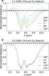 |
Fig. 6 Normalised radiance centred on the 9.6 µm O3 features, for selected phase angles of the 1:1 SOR (a) and 3:2 SOR (b). We fit the continuum data (8–9.15 and 10.15–12.2 µm) with a quadratic polynomial and normalise the radiance. This approach allows us to isolate the O3 feature as a function of orbital phase angle, illustrating the change from absorption to emission for the 1:1 SOR and the generally stronger absorption features for the 3:2 SOR. |
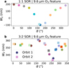 |
Fig. 7 Equivalent width (Wλ) as calculated by Eq. (5) as a function of the orbital phase angle θ, for the 1:1 SOR (a) and 3:2 SOR (b). The colours correspond to the curves shown in Fig. 6 and we separate the two orbits of the 3:2 SOR with distinct markers. The evolution of Wλ with θ shows how different orbits provide distinct temporal variations in biosignatures, attributed to viewing geometry and seasonality. |
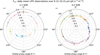 |
Fig. 8 Simulated daily observations of Proxima Centauri b for one orbit in the 1:1 SOR (left) and two orbits in the 3:2 SOR (right) with LIFE, averaged over wavelengths in the range 9.15–10.15 µm to probe spatial and temporal variations in the O3 feature. For the 1:1 SOR, the daily averaged fluxes are spread over 32.18◦ corresponding to the phase angle shift per day. For the eccentric 3:2 SOR, the daily phase angle shift varies, as shown by the varying arcs of the measurements. The two orbits of the 3:2 SOR are shown by circles and squares, respectively. |
4 Discussion
4.1 Prospects for atmospheric characterisation with LIFE
The synthetic observations of Proxima Centauri b demonstrate that MIR spectroscopy with LIFE confidently detects atmospheric molecules such as CO2, H2O, and O3 on rocky exoplanets, agreeing with Konrad et al. (2022) and Alei et al. (2022). Molecular absorption features and continuum emission enable the differentiation between different SORs, as shown here for 1:1 and 3:2 SORs, given an appropriate phase angle or temporal coverage of the planetary orbits. This spectral variability is a powerful tool to infer planetary rotation states and atmospheric dynamics. While O3 remains a key biosignature candidate, its interpretation is complicated by plausible abiotic production pathways on M-dwarf planets through photochemical processes (e.g. Hu et al. 2012; Domagal-Goldman et al. 2014; Tian et al. 2014; Harman et al. 2015), underscoring the need for contextual understanding. The relation between O3 and O2 depends on their respective abundances and varies with stellar type and abundances of other trace gases such as N2O and CH4 (Kozakis et al. 2022; Kozakis et al. 2025a,b). Spatial and temporal variations in O3 abundances and spectral features further complicate the derivation of O2 abundances from O3, and necessitate a comprehensive understanding of the planetary environment driving O3 variability. The combined detection of O3 and CH4 in exoplanet spectra presents a more robust biosignature (e.g. Schwieterman et al. 2018) and future work should assess the coupled spatial and temporal evolution of O3 and CH4 and the resulting spectral variability.
Our results demonstrate LIFE’s strengths in resolving spatial and temporal variations in atmospheric composition and temperature. Firstly, LIFE can reveal circulation patterns: planets in synchronous rotation (1:1 SOR) feature notable phase-dependent flux changes related to the eastward advection of the substellar cloud deck (Carone et al. 2015; Haqq-Misra et al. 2018; Sergeev et al. 2022b). These are detectable by LIFE by comparing planet fluxes at phase angles around 90◦ to fluxes around 270◦. Our analysis shows that variations in the equivalent width of O3 features (Wλ) for the 3:2 SOR are similar to the seasonal variability on Earth (∼5%; Mettler et al. 2023). Exoplanets in 1:1 SOR display much larger variability, including transitions from absorption to emission in O3 features when the nightside comes into view. The disappearance of O3 features at night-side phases agrees with Earth observations (Mettler et al. 2023) showing O3 and CO2 detection challenges for viewing angles centred on the polar regions. Hearty et al. (2009) note that the polar viewing angles can also produce emission features in O3 and water vapour arising due to temperature inversions, similar to the nightside viewing angles for the 1:1 SOR here. This clearly illustrates that spatial variability is significant for synchronous exoplanets, and phase-resolved observations can therefore reveal the 3D thermal structure. We find that phase angle degeneracies between different SORs persist without full phase coverage, necessitating phase-resolved observations rather than single snapshot spectra.
Due to the coupled impact of temperature, cloud, and ozone distributions, the interpretation of O3 variability is inherently tied to correctly interpreting the temperature and cloud distributions and necessitates a 4D modelling context. Since Wλ (Fig. 7) calculates the strength of the O3 feature relative to the continuum signal, it contains information on both the O3 distribution and the atmospheric structure. The predicted phase evolution and periodicity from 4D CCMs can further limit the number of possible degeneracies. Previous studies have shown that vertically constant temperature profiles, gaseous abundances, and non-patchy cloud profiles in retrievals bias the retrieved posteriors (in the context of LIFE, see Alei et al. 2022; Mettler et al. 2024; Konrad et al. 2024). Including physically motivated profiles for these parameters enables accurate retrievals of P–T structure, H2O and cloud profiles, and gaseous abundances from Earth’s thermal emission spectrum (Konrad et al. 2024), and will be essential for capturing the spatial and temporal variability predicted in this study. Future work should conduct a dedicated retrieval of phase-resolved synthetic LIFE spectra for exoplanets in SORs, including such physically motivated vertical profiles.
The interpretation of spatial and temporal variations is also crucial for inferring potentially habitable environments. Planets in 3:2 SOR show higher planet fluxes and moderated temporal variability due to eccentricity-driven heating and weakened dayside cloud feedback (Colose et al. 2021; Yang et al. 2013). Conversely, planets in 1:1 SOR maintain more static physical and chemical environments, with stronger spatial gradients. On planets in 1:1 SOR, habitability is plausible in the terminator regions (Shields et al. 2016; Lobo et al. 2023), but stronger cycling of UV radiation, temperature, and wet-dry phases thought critical for life’s origin and prevalence (Pearce et al. 2017; Del Genio et al. 2019) appear more prominent for 3:2 SORs. Water vapour spectral features and continuum variations modulated by clouds can serve as proxies for these surface wet-dry cycles.
We note that the reference architecture of LIFE has evolved from the setup assumed in this study (Table 2), most notably in terms of sensitivity (aperture diameter) and spectral resolution. Recent simulations of the optimal LIFE configuration point towards larger aperture sizes (F. Dannert et al., private comm.). For our analysis, this implies that the quality of spectra as presented in Figs. 4, 5, and 8 could be achieved with shorter observation times, or, conversely, that maintaining 24-hour integrations would yield even higher sensitivity for daily physical and chemical characterisation of Proxima Centauri b. Moreover, the planet’s small angular separation (∼60 mas) ensures that the reduction in field-of-view taper associated with a larger aperture will not affect the observations (Hansen et al., in prep.). Finally, an increased spectral resolution of R = 100 (Konrad et al. 2024) would further enhance spectral characterisation and can, if necessary, be downsampled to R = 50.
The synthetic observations we generated using LIFESIM consider astrophysical noise. In a realistic observing campaign, instrument systematic noise can induce offsets in the measured spectra, for example through temporal variability of the null floor from instrument perturbations, which in turn can mask the effects of atmospheric variability. Recent LIFE-focused studies have begun to quantify what this means for the instrument design of LIFE (Dannert et al. 2025; Huber et al. 2025; Rutten et al. in prep.), demonstrating that post-processing techniques such as data whitening can substantially mitigate these additional noise contributions (Huber et al. 2025). We therefore expect that, while systematic null-floor variability may reduce absolute sensitivity to some degree, the impact on the inter-phase differences and diagnostic comparisons presented in this study can be mitigated.
4.2 Limitations to the model configuration
The predicted spectral differences between SORs depend on the assumed surface conditions, atmospheric composition and pressure, and atmospheric circulation regimes. Fujii et al. (2026) analyse spatial gradients and their effects on MIR spectra of rocky exoplanets in 1:1 SOR for diverse surface scenarios. Global slab oceans tend to homogenise phase-dependent continuum emission, whereas atmospheres without oceans exhibit enhanced phase variability despite the presence of water vapour (Fujii et al. 2026). Since our simulations concern global slab oceans, the predicted MIR variability might be enhanced in scenarios with more land coverage. On the other hand, Del Genio et al. (2019) show that global dynamic oceans (i.e. including ocean heat transport) homogenise temperature distributions. Nevertheless, zonal asymmetries in geopotential height for dynamic ocean scenarios suggest that circulation-driven ozone asymmetries persist. Combining both arguments, an assumed global slab ocean may be a middle case in terms of MIR variability, with enhanced land coverage enhancing spectral variability and global dynamic oceans reducing it. The inclusion of orography affects atmospheric circulation and thus the ozone distribution (Bhongade et al. 2024). Future work should elucidate the robustness of predicted O3, H2O, and CO2 variability for varying land cover and dynamic oceans, for example using an efficient two-layer dynamical slab ocean model (Bhatnagar et al. 2025).
Exoplanets in 1:1 SOR exhibit specific circulation regimes depending on the orbital period (Carone et al. 2015; Noda et al. 2017; Haqq-Misra et al. 2018). Moreover, for planets close to regime transitions, model parameterisations can flip the regime (Sergeev et al. 2020), or planets can exhibit bistability (Sergeev et al. 2022b). The circulation regime is crucial to the 4D distributions of, for example, temperature, humidity, and photochemical species. However, the atmosphere of Proxima Centauri b is comparatively stable against regime changes. Carone et al. (2018) show in their figure 1 that Proxima Centauri b falls in the weak superrotation or single jet regime. Compared to this, TRAPPIST-1 e falls on the boundary between two circulation regimes, making it particularly susceptible to regime changes (Sergeev et al. 2022b). For Proxima b, a different convection parameterisation scheme also does not change the circulation regime (Sergeev et al. 2020). Nevertheless, the sensitivity of the simulated distributions can be further evaluated against diverse landmasses (Lewis et al. 2018) and tidal heating (Colose et al. 2021).
Our simulations assume a 1 bar pre-industrial Earth-like atmosphere of N2, O2, and CO2 as a fiducial case. However, we note that the results presented will be affected by different atmospheric compositions and pressures. Turbet et al. (2016) explore the effects of diverse atmospheric scenarios on the climate of Proxima b. They show that the zonal variations in surface temperature for a 1:1 SOR, including the high-latitude gyres as the coldest regions on the planet, hold for atmospheres with and without water vapour as well as pressure variations of 1–20 bar. Nevertheless, varying gyre positions and prominence potentially affect the zonal variations. The 3:2 SOR, in this case without eccentricity, consistently displays latitudinal variations, but enhanced CO2 abundances lower the temperature contrasts. Although investigations of ozone photochemistry are mostly limited to pre-industrial Earth-like conditions, investigations of the ozone distributions on exoplanets in 1:1 SOR with lower O2 levels (down to 1% or 0.1% present atmospheric level) show that the zonal variations persist (Braam et al. 2023; Cooke et al. 2023a).
Mak et al. (2024) use the UM to simulate the atmosphere of TRAPPIST-1 e in 1:1 SOR, with varying CO2/CH4 partial pressures as well as prescribed haze layers corresponding to the CH4 levels, in a background of N2. For increasing CO2 levels, the circulation regime and zonal temperature variations persist, although temperature contrasts decrease. Varying CH4 levels can change the circulation regime, substantially affecting the zonal temperature variations, but higher CH4 abundances cool the surface. When hazes are included, further surface cooling is predicted, along with enhanced zonal temperature variations (Mak et al. 2024). As noted by Braam et al. (2023), the circulation-driven chemical distributions likely hold for any chemical compounds resulting from stratospheric photochemistry. Therefore, photochemical hazes or other products from methane photodissociation may show similar spatial variations. The 4D aspects of this photochemistry need further study, including their MIR observability and variability.
4.3 Abiotic scenarios for seasonally varying biosignatures
Seasonally varying biosignatures are considered among the strongest indicators of life (Olson et al. 2018; Schwieterman et al. 2018). Clouds modulate spectral intensities and variability amplitudes (Tinetti et al. 2006a; Des Marais et al. 2002; Kitzmann et al. 2011), but O3 location above cloud layers mitigates this effect. However, O3 features tend to saturate, limiting precise abundance constraints despite phase-dependent flux changes. The variations in Wλ of O3 translate into small and big variations for predicted LIFE spectra of the 3:2 and 1:1 SOR, and such variations would be further enhanced if landmasses were included (Mettler et al. 2023). Within typical error bars, the spatial and temporal variations in O3 are detectable, mimicking signals due to seasonally varying biosignatures (Olson et al. 2018; Schwieterman et al. 2018). As noted before, abiotic pathways to O3 production exist on planets around M-dwarfs (e.g. Hu et al. 2012; Domagal-Goldman et al. 2014; Tian et al. 2014; Harman et al. 2015). Therefore, such ‘abiotic’ spatial and temporal variations due to orbital geometry or internal atmospheric variability (see also Cohen et al. 2023; Cooke et al. 2023b; Braam et al. 2025) are possible for tidally locked planets and potentially appear as false positives in LIFE spectra. Interpreting the spectra alongside 4D model predictions can circumvent the ambiguity by providing the expected periodicity of abiotic variability.
4.4 Observational recommendations for LIFE
We obtain little insight into key biosignatures and their variability in the 4–6.5 µm spectral range, given the predicted noise for LIFE observations of Proxima Centauri b. This is partly due to baseline optimisation focused on longer wavelengths and the total planetary flux. Alternatively, LIFE observations can change the baseline to optimise for shorter wavelengths, both for Proxima Centauri b or other targets (not shown). Wavelengths >16 µm, on the other hand, are affected by water vapour features with statistically significant variability for the 1:1 SOR and should be prioritised. Enhanced spectral resolution near the 9.6 µm O3 band appears unnecessary given the detectable variability effects in O3 for the 1:1 SOR. The predicted signal-to-noise ratio allows us to confidently detect or rule out O3 and water vapour variability around Proxima Centauri b, provided observations are taken at multiple phase angles and not as snapshot spectra. The detection of variability and distinction between SORs is, in essence, a comparison of timescales. Observation times must be balanced against variability timescales: longer integrations will improve S/N but can lead to unresolved variability by averaging over phase angles, potentially hiding dynamic features. Careful observation planning should therefore include a determination of optimal phase angle coverage given dynamical and (photo)chemical timescales.
Studying the phase dependence of exoplanetary signals observed with LIFE thus also plays an important role in the ongoing definition of the observing strategy. In current yield studies such as Quanz et al. (2022); Kammerer et al. (2022), planets are assumed to be static with randomised orbital phase angles, i.e. not significantly changing throughout the observation. Such snapshot observations at random phase angles, used to identify potential rocky planet candidates during the detection phase of LIFE, could lead to confusion about the nature of the planet (e.g. missing O3 signature, how to fit temperature and/or blackbody). The results presented here can be used to optimise and refine the detection strategy by guiding the timing of multiple visits for confirming detected planet candidates and informing the transition from the detection to the characterisation phase (e.g. by excluding planets exhibiting large phase variations). Most of LIFE’s characterisation observations (cf. Konrad et al. 2022; Alei et al. 2022) require long integration times and, depending on planetary spin rates and tidal locking, need to take into account the 4D structure of this problem, i.e. that they average over changing phase angles.
Time integrations for LIFE observations of any planet include unresolved spatial and temporal variations, but the orbital period and distance from Earth make Proxima Centauri b a golden target for LIFE (Angerhausen et al. 2024). By combining daily average climate model output and daily observations with LIFE, we demonstrate LIFE’s potential to provide daily characterisation of the physical and chemical state of the atmosphere of Proxima Centauri b. Planets on shorter orbital periods face larger daily phase angle changes and therefore lose spatial and temporal resolution in LIFE observations. Temperate planets on longer orbital periods around brighter stars may still be tidally locked into SORs within their lifetime (Barnes 2017). We perform initial tests that suggest that analogous variability in MIR spectra is accessible around brighter stars, but requires longer observations (see Appendix B). As such, there will be a substantial number of exoplanetary systems within ∼5–7 parsec accessible for LIFE characterisation in a similar manner. For instance, Angerhausen et al. (2024) showed that LIFE has an expected yield of about a dozen HZ planets in late-type systems and a handful in FGK-host systems within 6 pcs. For planets on longer periods around brighter stars, longer observations may cover phase angle variations similar to those in our study, thus providing similar spatial and temporal resolution. Nevertheless, the associated differences in host star spectral type, orbital configuration, atmospheric dynamics, and atmospheric chemistry will modulate the signals observed by LIFE, motivating broader modelling efforts of 4D atmospheric chemistry for planets around K- and G-type stars with varying orbital periods.
In this study, we used an intermediate inclination (∼70◦) to determine the effects of spatial and temporal variations on emission spectra with LIFE, reflecting estimates for Proxima Centauri b and other 3D climate modelling studies (Turbet et al. 2016; Kane et al. 2017; Boutle et al. 2017; Braam et al. 2025). For this inclination, Proxima Centauri b stays within the optimal modulation efficiency range of LIFE. However, other inclinations are possible, where targets such as Proxima Centauri b temporarily leave the optimal modulation efficiency range. Additionally, this would change the planetary mass (and radius) of Proxima Centauri b through the M sin(i) = 1.27 M⊕ dependence. A (significantly) smaller inclination modulates the phase variability, but previous work has shown that emission spectra are less sensitive than reflection spectra (Turbet et al. 2016; Boutle et al. 2017). Future work should investigate inclination variations to further constrain LIFE’s ability to characterise spatial and temporal variations on terrestrial exoplanets and to determine whether temporarily leaving the optimal modulation efficiency range of LIFE affects this characterisation. We note that inferences on planetary atmosphere and surface conditions from spectra depend on model assumptions (Paradise et al. 2022; Fauchez et al. 2022), motivating further development of coupled 4D CCMs and retrieval methods considering spatial-temporal variability.
5 Conclusions
This study combines comprehensive 4D climate-chemistry modelling with synthetic MIR observations to investigate LIFE’s capability to characterise spatial and temporal variations in the atmosphere of Proxima Centauri b and similar nearby exoplanets. Our key findings are as follows:
LIFE enables daily MIR characterisation of atmospheric composition and variability on Proxima Centauri b, confidently distinguishing between different SOR scenarios through observable differences in O3, water vapour, and temperature signatures;
The synchronous (1:1) SOR produces strong hemispheric chemical and thermal contrasts, with detectable phase-dependent O3 features and temperature inversions on the nightside, while the eccentric (3:2) SOR yields a more homogeneous atmosphere and enhanced global flux due to variable stellar irradiation;
Simulated LIFE observations demonstrate that 4D (spatial and temporal) atmospheric variability in rocky exoplanets can be resolved, allowing the discrimination of dynamical and chemical regimes and providing detailed insight into atmospheric circulation mechanisms, such as the advection of cloud decks and O3 accumulation;
The study highlights that phase-dependent molecular features can act as false positives for seasonal biosignatures, in the case of abiotic O2 and O3 build-up, emphasising the need for robust interpretation strategies that account for orbital and planetary context when assessing biosignatures on M-dwarf planets;
The results advocate further 4D modelling efforts and optimised observing strategies for LIFE and similar missions, suggesting that dozens of exoplanets within 7 parsec may be accessible for 4D daily characterisation, advancing the search for biosignatures and our understanding of terrestrial planet atmospheres.
Acknowledgements
We thank Thomas Fauchez, Vincent Kofman, and Geronimo Villanueva for advice on generating emission spectra from a 3D model using PSG. We thank Andrea Fortier, Felix Dannert, Philipp Huber and Jonah Hansen for helpful discussions about LIFESIM, baselines and instrument requirements in general. We thank Felix Dannert, Eleonora Alei, and Sascha Quanz for valuable feedback on the manuscript. We also thank Yuka Fujii and the LIFE Science Team for helpful discussions. We are grateful to the anonymous reviewer whose comments helped to significantly improve the manuscript. MB appreciates support from a CSH Fellowship. For the CCM simulations, we gratefully acknowledge the use of the MONSooN2 system, a collaborative facility supplied under the Joint Weather and Climate Research Programme, a strategic partnership between the UK Met Office and the Natural Environment Research Council. Our simulations were performed as part of the project space “Using UKCA to investigate atmospheric composition on extra-solar planets (ExoChem).”
References
- Alei, E., Konrad, B. S., Angerhausen, D., et al. 2022, A&A, 665, A106 [NASA ADS] [CrossRef] [EDP Sciences] [Google Scholar]
- Alei, E., Quanz, S. P., Konrad, B., et al. 2024, A&A, 689, A245 [NASA ADS] [CrossRef] [EDP Sciences] [Google Scholar]
- Angerhausen, D., Ottiger, M., Dannert, F., et al. 2023, Astrobiology, 23, 183 [NASA ADS] [CrossRef] [Google Scholar]
- Angerhausen, D., Pidhorodetska, D., Leung, M., et al. 2024, AJ, 167, 128 [NASA ADS] [CrossRef] [Google Scholar]
- Anglada-Escudé, G., Amado, P. J., Barnes, J., et al. 2016, Nature, 536, 437 [Google Scholar]
- Archibald, A. T., O’Connor, F. M., Abraham, N. L., et al. 2020, GMD, 13, 1223 [Google Scholar]
- Barnes, R. 2017, Celest. Mech. Dyn. Astron., 129, 509 [Google Scholar]
- Bhatnagar, S., Codron, F., Millour, E., et al. 2025, EGUsphere, 2025, 1 [Google Scholar]
- Bhongade, A., Marsh, D. R., Sainsbury-Martinez, F., & Cooke, G. 2024, ApJ, 977, 96 [Google Scholar]
- Boutle, I. A., Mayne, N. J., Drummond, B., et al. 2017, A&A, 601, A120 [NASA ADS] [CrossRef] [EDP Sciences] [Google Scholar]
- Braam, M., Palmer, P. I., Decin, L., Cohen, M., & Mayne, N. J. 2023, MNRAS, 526, 263 [NASA ADS] [CrossRef] [Google Scholar]
- Braam, M., Palmer, P. I., Decin, L., et al. 2022, MNRAS, 517, 2383 [NASA ADS] [CrossRef] [Google Scholar]
- Braam, M., Palmer, P. I., Decin, L., et al. 2025, PSJ, 6, 5 [Google Scholar]
- Carone, L., Keppens, R., & Decin, L. 2015, MNRAS, 453, 2412 [Google Scholar]
- Carone, L., Keppens, R., Decin, L., & Henning, T. 2018, MNRAS, 473, 4672 [NASA ADS] [CrossRef] [Google Scholar]
- Carrión-González, Ó., Kammerer, J., Angerhausen, D., et al. 2023, A&A, 678, A96 [NASA ADS] [CrossRef] [EDP Sciences] [Google Scholar]
- Catling, D. C., Krissansen-Totton, J., Kiang, N. Y., et al. 2018, Astrobiology, 18, 709 [NASA ADS] [CrossRef] [Google Scholar]
- Chen, H., Wolf, E. T., Kopparapu, R., Domagal-Goldman, S., & Horton, D. E. 2018, ApJ, 868, L6 [NASA ADS] [CrossRef] [Google Scholar]
- Chen, H., Wolf, E. T., Zhan, Z., & Horton, D. E. 2019, ApJ, 886, 16 [NASA ADS] [CrossRef] [Google Scholar]
- Chen, H., Zhan, Z., Youngblood, A., et al. 2021, NatAs, 5, 298 [Google Scholar]
- Chen, H., Li, G., Paradise, A., & Kopparapu, R. K. 2023, ApJ, 946, L32 [NASA ADS] [CrossRef] [Google Scholar]
- Chen, H., De Luca, P., Hochman, A., & Komacek, T. D. 2025, AJ, 170, 40 [Google Scholar]
- Cohen, M., Bollasina, M. A., Sergeev, D. E., Palmer, P. I., & Mayne, N. J. 2023, PSJ, 4, 68 [Google Scholar]
- Colose, C. M., Haqq-Misra, J., Wolf, E. T., et al. 2021, ApJ, 921, 25 [NASA ADS] [CrossRef] [Google Scholar]
- Cooke, G., Marsh, D., Walsh, C., & Youngblood, A. 2023a, ApJ, 959, 45 [NASA ADS] [CrossRef] [Google Scholar]
- Cooke, G. J., Marsh, D. R., Walsh, C., Rugheimer, S., & Villanueva, G. L. 2023b, MNRAS, 518, 206 [Google Scholar]
- Cooke, G., Marsh, D., Walsh, C., & Sainsbury-Martinez, F. 2024, PSJ, 5, 168 [Google Scholar]
- Dannert, F. A., Ottiger, M., Quanz, S. P., et al. 2022, A&A, 664, A22 [NASA ADS] [CrossRef] [EDP Sciences] [Google Scholar]
- Dannert, F. A., Huber, P. A., Birbacher, T., et al. 2025, AJ, 170, 193 [Google Scholar]
- Del Genio, A. D., Way, M. J., Amundsen, D. S., et al. 2019, Astrobiology, 19, 99 [Google Scholar]
- Des Marais, D. J., Harwit, M. O., Jucks, K. W., et al. 2002, Astrobiology, 2, 153 [NASA ADS] [CrossRef] [Google Scholar]
- Dobrovolskis, A. R. 2007, Icarus, 192, 1 [NASA ADS] [CrossRef] [Google Scholar]
- Domagal-Goldman, S. D., Segura, A., Claire, M. W., Robinson, T. D., & Meadows, V. S. 2014, ApJ, 792, 90 [CrossRef] [Google Scholar]
- Edwards, J. M., & Slingo, A. 1996, QJRMS, 122, 689 [Google Scholar]
- Fauchez, T. J., Villanueva, G. L., Sergeev, D. E., et al. 2022, PSJ, 3, 213 [Google Scholar]
- Fauchez, T. J., Villanueva, G. L., Kofman, V., Suissa, G., & Kopparapu, R. K. 2025, A & C, 100982 [Google Scholar]
- Fujii, Y., Angerhausen, D., Deitrick, R., et al. 2018, Astrobiology, 18, 739 [NASA ADS] [CrossRef] [Google Scholar]
- Fujii, Y., Angerhausen, D., Matsuo, T., & Wolf, E. T. 2026, ApJ, in press, https://doi.org/10.3847/1538-3881/ae367b [Google Scholar]
- Glauser, A. M., Quanz, S. P., Hansen, J., et al. 2024, in Optical and Infrared Interferometry and Imaging IX, 13095, SPIE, 354 [Google Scholar]
- Goldreich, P., & Peale, S. 1966, AJ, 71, 425 [NASA ADS] [CrossRef] [Google Scholar]
- Guzewich, S. D., Lustig-Yaeger, J., Davis, C. E., et al. 2020, ApJ, 893, 140 [Google Scholar]
- Gómez-Leal, I., Pallé, E., & Selsis, F. 2012, ApJ, 752, 28 [CrossRef] [Google Scholar]
- Haqq-Misra, J., Wolf, E. T., Joshi, M., Zhang, X., & Kopparapu, R. K. 2018, ApJ, 852, 67 [NASA ADS] [CrossRef] [Google Scholar]
- Harman, C., Schwieterman, E., Schottelkotte, J. C., & Kasting, J. 2015, ApJ, 812, 137 [NASA ADS] [CrossRef] [Google Scholar]
- Hearty, T., Song, I., Kim, S., & Tinetti, G. 2009, ApJ, 693, 1763 [Google Scholar]
- Hochman, A., De Luca, P., & Komacek, T. D. 2022, ApJ, 938, 114 [Google Scholar]
- Hu, R., Seager, S., & Bains, W. 2012, ApJ, 761, 166 [CrossRef] [Google Scholar]
- Huber, P. A., Dannert, F. A., Laugier, R., et al. 2025, AJ, 170, 227 [Google Scholar]
- Kammerer, J., Quanz, S. P., Dannert, F., & LIFE Collaboration 2022, A&A, 668, A52 [NASA ADS] [CrossRef] [EDP Sciences] [Google Scholar]
- Kane, S. R., Gelino, D. M., & Turnbull, M. C. 2017, AJ, 153, 52 [Google Scholar]
- Kitzmann, D., Patzer, A. B. C., von Paris, P., Godolt, M., & Rauer, H. 2011, A&A, 531, A62 [NASA ADS] [CrossRef] [EDP Sciences] [Google Scholar]
- Kofman, V., Villanueva, G. L., Fauchez, T. J., et al. 2024, PSJ, 5, 197 [Google Scholar]
- Konrad, B. S., Alei, E., Quanz, S. P., et al. 2022, A&A, 664, A23 [NASA ADS] [CrossRef] [EDP Sciences] [Google Scholar]
- Konrad, B. S., Alei, E., Quanz, S. P., et al. 2023, A&A, 673, A94 [NASA ADS] [CrossRef] [EDP Sciences] [Google Scholar]
- Konrad, B. S., Quanz, S. P., Alei, E., & Wordsworth, R. 2024, ApJ, 975, 13 [Google Scholar]
- Kozakis, T., Mendonça, J. M., & Buchhave, L. A. 2022, A&A, 665, A156 [NASA ADS] [CrossRef] [EDP Sciences] [Google Scholar]
- Kozakis, T., Mendonça, J. M., Buchhave, L. A., & Lara, L. M. 2025a, A&A, 699, A247 [NASA ADS] [CrossRef] [EDP Sciences] [Google Scholar]
- Kozakis, T., Mendonça, J. M., Buchhave, L. A., & Lara, L. M. 2025b, A&A, 701, A254 [NASA ADS] [CrossRef] [EDP Sciences] [Google Scholar]
- Leung, M., Tsai, S.-M., Schwieterman, E. W., Angerhausen, D., & Hansen, J. 2025, ApJ, 982, L2 [Google Scholar]
- Lewis, N. T., Lambert, F. H., Boutle, I. A., et al. 2018, ApJ, 854, 171 [NASA ADS] [CrossRef] [Google Scholar]
- Lobo, A. H., Shields, A. L., Palubski, I. Z., & Wolf, E. 2023, ApJ, 945, 161 [NASA ADS] [CrossRef] [Google Scholar]
- Luo, Y., Hu, Y., Yang, J., Zhang, M., & Yung, Y. L. 2023, PNAS, 120, e2309312120 [Google Scholar]
- Mak, M. T., Sergeev, D. E., Mayne, N., et al. 2024, MNRAS, 529, 3971 [Google Scholar]
- Manners, J., Edwards, J. M., Hill, P., & Thelen, J.-C. 2021, SOCRATES (Suite Of Community RAdiative Transfer codes based on Edwards and Slingo) Technical Guide [Google Scholar]
- Mayne, N. J., Baraffe, I., Acreman, D. M., et al. 2014, GMD, 7, 3059 [Google Scholar]
- Meadows, V. S., Reinhard, C. T., Arney, G. N., et al. 2018, Astrobiology, 18, 630 [Google Scholar]
- Mettler, J.-N., Quanz, S. P., Helled, R., Olson, S. L., & Schwieterman, E. W. 2023, ApJ, 946, 82 [Google Scholar]
- Mettler, J.-N., Konrad, B. S., Quanz, S. P., & Helled, R. 2024, ApJ, 963, 24 [NASA ADS] [CrossRef] [Google Scholar]
- Mueller, M. 1995, AcPPA, 88, S-49 [Google Scholar]
- Noda, S., Ishiwatari, M., Nakajima, K., et al. 2017, Icarus, 282, 1 [Google Scholar]
- Olson, S. L., Schwieterman, E. W., Reinhard, C. T., et al. 2018, ApJ, 858, L14 [NASA ADS] [CrossRef] [Google Scholar]
- Paradise, A., Menou, K., Lee, C., & Fan, B. L. 2022, MNRAS, 512, 3616 [Google Scholar]
- Pearce, B. K., Pudritz, R. E., Semenov, D. A., & Henning, T. K. 2017, PNAS, 114, 11327 [NASA ADS] [CrossRef] [Google Scholar]
- Pierrehumbert, R. T., & Hammond, M. 2019, AnRFM, 51, 275 [Google Scholar]
- Quanz, S. P., Ottiger, M., Fontanet, E., et al. 2022, A&A, 664, A21 [NASA ADS] [CrossRef] [EDP Sciences] [Google Scholar]
- Renaud, J. P., Henning, W. G., Saxena, P., et al. 2021, PSJ, 2, 4 [Google Scholar]
- Ridgway, R. J., Zamyatina, M., Mayne, N. J., et al. 2023, MNRAS, 518, 2472 [Google Scholar]
- Schwieterman, E. W., Kiang, N. Y., Parenteau, M. N., et al. 2018, Astrobiology, 18, 663 [CrossRef] [Google Scholar]
- Sergeev, D. E., Lambert, F. H., Mayne, N. J., et al. 2020, ApJ, 894, 84 [NASA ADS] [CrossRef] [Google Scholar]
- Sergeev, D. E., Fauchez, T. J., Turbet, M., et al. 2022a, PSJ, 3, 212 [NASA ADS] [Google Scholar]
- Sergeev, D. E., Lewis, N. T., Lambert, F. H., et al. 2022b, PSJ, 3, 214 [NASA ADS] [Google Scholar]
- Shields, A. L., Ballard, S., & Johnson, J. A. 2016, PhR, 663, 1 [Google Scholar]
- Smart, W. M. 1944, Text-book on Spherical Astronomy (The University Press) [Google Scholar]
- Telford, P. J., Abraham, N. L., Archibald, A. T., et al. 2013, GMD, 6, 161 [Google Scholar]
- Tian, F., France, K., Linsky, J. L., Mauas, P. J., & Vieytes, M. C. 2014, E & PSL, 385, 22 [Google Scholar]
- Tinetti, G., Meadows, V. S., Crisp, D., et al. 2006a, Astrobiology, 6, 34 [Google Scholar]
- Tinetti, G., Meadows, V. S., Crisp, D., et al. 2006b, Astrobiology, 6, 881 [Google Scholar]
- Turbet, M., Leconte, J., Selsis, F., et al. 2016, A&A, 596, A112 [NASA ADS] [CrossRef] [EDP Sciences] [Google Scholar]
- Villanueva, G. L., Liuzzi, G., Faggi, S., et al. 2022, Fundamentals of the Planetary Spectrum Generator [Google Scholar]
- Villanueva, G. L., Smith, M. D., Protopapa, S., Faggi, S., & Mandell, A. M. 2018, JQSRT, 217, 86 [NASA ADS] [CrossRef] [Google Scholar]
- Walters, D., Baran, A. J., Boutle, I., et al. 2019, GMD, 12, 1909 [Google Scholar]
- Way, M. J., & Georgakarakos, N. 2017, ApJ, 835, L1 [Google Scholar]
- Yang, J., Cowan, N. B., & Abbot, D. S. 2013, ApJ, 771, L45 [Google Scholar]
- Yates, J. S., Palmer, P. I., Manners, J., et al. 2020, MNRAS, 492, 1691 [NASA ADS] [CrossRef] [Google Scholar]
Appendix A Hemispheric mean climate-chemistry model output
In Tables A.1 and A.2, we present the hemispheric mean climate and chemistry diagnostics, as a function of phase angle and averaged over the observed hemisphere. These are visualised in Fig. 2.
Hemispheric means across the observed hemisphere of Proxima Centauri b in 1:1 SOR.
Hemispheric means across the observed hemisphere of Proxima Centauri b in 3:2 SOR.
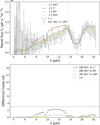 |
Fig. B.1 Same as Fig. 4, but for an M3V system at 5 pcs and 4 days of observation time. We note that the scale on the flux axis is one order of magnitude smaller. The grey area represents the 1σ sensitivity; the dark grey error bars show an individual simulated observation. Lower panel: Statistical significance of the detected differences between different phases. |
Appendix B Generalisation to other targets
As mentioned in Sect. 4.4, we performed initial tests to investigate whether analogous variability is accessible around brighter stars. We use the 4D distributions from the Proxima Centauri b configurations (Sect. 3.1) to create synthetic LIFE spectra for exoplanets in the HZ of brighter stars. Figure B.1 shows the phase angle dependence of these spectra around an M3V star (3439 K, 0.361 RSun, 0.127 AU) at 5 pcs. Such targets represent a more typical early-type LIFE target (Angerhausen et al. 2024; Leung et al. 2025), with dozens of observable planets at favourable inclination. From Kepler’s third law, such an exo-planet covers an orbital phase angle change of ∼32◦ in four days, which we take as the observation time. Whilst the 4D variations are not as clearly distinguishable as in the golden target case of Proxima Centauri b, phase angle variations are of the same order of magnitude as the noise floor visible and may still provide a source of confusion when taking snapshot spectra. We note that these tests are not physically or chemically consistent, as the distinct orbital, dynamical, and photochemical timescales likely produce a different 4D atmospheric state. A more detailed analysis of these early-type LIFE targets is presented in Fujii et al. (2026). We suggest that future work focus on self-consistently simulating the 4D atmospheric chemistry and exploring observational prospects for these targets. A crucial aspect will be the comparison of orbital and chemical timescales, to investigate whether longer observations still probe 4D chemistry or whether these smooth out any variations.
All Tables
True anomaly ν(t) and orbital phase angle θ(t) for Proxima Centauri b in a 1:1 and 3:2 SOR.
Overview of simulation parameters used in LIFESIM, following Quanz et al. (2022) or Angerhausen et al. (2023).
Hemispheric means across the observed hemisphere of Proxima Centauri b in 1:1 SOR.
Hemispheric means across the observed hemisphere of Proxima Centauri b in 3:2 SOR.
All Figures
|
Fig. 1 Observed hemispheric distributions as a function of θ(t) for the 1:1 SOR (top) and the 3:2 SOR with an eccentricity of 0.3 (bottom): surface temperature (blue-red), vertically integrated water vapour or H2O (g) column density (white–blue), vertically integrated total cloud path (white-grey), and vertically integrated O3 column density (dark blue– yellow). The longitude of perihelion of the 3:2 SOR is at 102.94◦. For both SORs, we use four extreme cases of θ(t) (see Table 1). The distributions vary spatially and temporally, illustrating the orbital evolution of climate and chemistry, as well as the effects of viewing geometry. |
| In the text | |
|
Fig. 2 Phase angle evolution of the hemispheric means across the observed hemisphere of Proxima Centauri b in 1:1 SOR (navy) and 3:2 SOR (orange), for the quantities shown in Fig. 1 and |
| In the text | |
|
Fig. 3 Simulated spectral radiance at the top of the atmosphere for Proxima Centauri b in (a) 1:1 SOR and (b) 3:2 SOR, for θ(t) as shown in Table 1. The spectra were created using PSG and the GlobES tool (see Sect. 2.2 for details). We also include blackbody curves at different temperatures for comparison and grey rectangles for important molecular and CIA features. For panel (b), the solid and dashed lines represent the first and second orbits around the host star, respectively, and together correspond to the length of a full day for the 3:2 SOR. |
| In the text | |
|
Fig. 4 Example simulated LIFE observation for the 1:1 resonance case (left) and 3:2 resonance case (right) assuming an integration time of 24 hours. The grey area represents the 1σ sensitivity; the dark grey error bars show an individual simulated observation. Lower panel: Statistical significance of the detected differences between different phases. |
| In the text | |
|
Fig. 5 Pairs of simulated LIFE spectra for the 1:1 SOR at similar distances from phase angles of 90 and 270◦, illustrating the effects of the atmospheric circulation. Panel a shows spectra for phase angles 98 and 265◦, panel b for 130 and 233◦, and panel c for 66 and 297◦. |
| In the text | |
|
Fig. 6 Normalised radiance centred on the 9.6 µm O3 features, for selected phase angles of the 1:1 SOR (a) and 3:2 SOR (b). We fit the continuum data (8–9.15 and 10.15–12.2 µm) with a quadratic polynomial and normalise the radiance. This approach allows us to isolate the O3 feature as a function of orbital phase angle, illustrating the change from absorption to emission for the 1:1 SOR and the generally stronger absorption features for the 3:2 SOR. |
| In the text | |
|
Fig. 7 Equivalent width (Wλ) as calculated by Eq. (5) as a function of the orbital phase angle θ, for the 1:1 SOR (a) and 3:2 SOR (b). The colours correspond to the curves shown in Fig. 6 and we separate the two orbits of the 3:2 SOR with distinct markers. The evolution of Wλ with θ shows how different orbits provide distinct temporal variations in biosignatures, attributed to viewing geometry and seasonality. |
| In the text | |
|
Fig. 8 Simulated daily observations of Proxima Centauri b for one orbit in the 1:1 SOR (left) and two orbits in the 3:2 SOR (right) with LIFE, averaged over wavelengths in the range 9.15–10.15 µm to probe spatial and temporal variations in the O3 feature. For the 1:1 SOR, the daily averaged fluxes are spread over 32.18◦ corresponding to the phase angle shift per day. For the eccentric 3:2 SOR, the daily phase angle shift varies, as shown by the varying arcs of the measurements. The two orbits of the 3:2 SOR are shown by circles and squares, respectively. |
| In the text | |
|
Fig. B.1 Same as Fig. 4, but for an M3V system at 5 pcs and 4 days of observation time. We note that the scale on the flux axis is one order of magnitude smaller. The grey area represents the 1σ sensitivity; the dark grey error bars show an individual simulated observation. Lower panel: Statistical significance of the detected differences between different phases. |
| In the text | |
Current usage metrics show cumulative count of Article Views (full-text article views including HTML views, PDF and ePub downloads, according to the available data) and Abstracts Views on Vision4Press platform.
Data correspond to usage on the plateform after 2015. The current usage metrics is available 48-96 hours after online publication and is updated daily on week days.
Initial download of the metrics may take a while.