| Issue |
A&A
Volume 707, March 2026
|
|
|---|---|---|
| Article Number | A283 | |
| Number of page(s) | 17 | |
| Section | Extragalactic astronomy | |
| DOI | https://doi.org/10.1051/0004-6361/202557861 | |
| Published online | 12 March 2026 | |
The imprint of AGN-driven outflows on the Circumgalactic Medium: The case of Lyα nebulae around high-z quasars
1
European Southern Observatory, Karl-Schwarzschild-Strasse 2, 85748 Garching bei München, Germany
2
Max-Planck-Institut für extraterrestrische Physik, Gießenbachstraße 1, 85748 Garching bei München, Germany
3
Centre for Astrophysics Research, University of Hertfordshire, Hatfield AL10 9AB, UK
4
Max-Planck-Institut für Astrophysik, Karl-Schwarzschild-Straße 1, 85748 Garching bei München, Germany
5
School of Mathematics, Statistics and Physics, Newcastle University, Newcastle upon Tyne NE1 7RU, UK
6
International Gemini Observatory/NSF NOIRLab, 670 N A’ohoku Place, Hilo Hawai’i 96720, USA
7
INAF – Osservatorio di Astrofisica e Scienza dello Spazio di Bologna, Via Gobetti 93/3, I-40129 Bologna, Italy
★ Corresponding author: This email address is being protected from spambots. You need JavaScript enabled to view it.
Received:
27
October
2025
Accepted:
3
February
2026
Abstract
Some cosmological hydrodynamical simulations predict that outflows driven by active galactic nuclei (AGN) play a key role in powering the Lyα nebulae observed around high-redshift quasars. In such simulations, AGN feedback seeded as powerful outflows leads to extended and luminous nebulae whose morphology and surface-brightness profiles accurately reproduce the observations, while suppressing AGN feedback leads to compact and faint nebulae. This link might arise from outflows opening up a channel for Lyα photons to escape from the galactic nucleus to the circumgalactic medium (CGM). The main aim of this paper is to test this theoretical prediction using observations, by comparing the physical properties of outflows and Lyα nebulae. We analyze integral-field unit data obtained with VLT/ERIS and GEMINI/GNIRS to trace the ionized gas in the interstellar medium (ISM) of a sample of six quasars at z ∼ 2 − 3, using the [O III] emission line. We detect powerful outflows in all the quasars of our sample, with velocities > 1500 km s−1 and kinetic energies ≳2 × 1043 erg s−1. Four of our quasars are spatially resolved and show signs of extended [O III] emission out to distances > 2 kpc from the central supermassive black hole. When excluding one outlier, we find a positive monotonic correlation between the outflow power and the Lyα nebulae size (ρ = 0.89, p = 0.03) and luminosity (ρ = 0.6, p = 0.28). Additionally, we find evidence of spatial alignment between the ionization cone and the inner and brightest regions of the Lyα nebula. Our results provide tentative evidence in support of the theoretical prediction that AGN-driven outflows at ISM scales open a low-optical-depth path for central Lyα photons to reach the CGM and create extended nebulae.
Key words: galaxies: active / galaxies: evolution / galaxies: halos / galaxies: high-redshift / quasars: emission lines
© The Authors 2026
 Open Access article, published by EDP Sciences, under the terms of the Creative Commons Attribution License (https://creativecommons.org/licenses/by/4.0), which permits unrestricted use, distribution, and reproduction in any medium, provided the original work is properly cited.
This article is published in open access under the Subscribe to Open model. This email address is being protected from spambots. You need JavaScript enabled to view it. to support open access publication.
1. Introduction
The influence of supermassive black hole (BH) activity on the evolution of its host galaxy has been extensively studied in the past decades (e.g., Kormendy & Ho 2013). It is widely accepted now that the BH and host galaxy properties are closely correlated, as evidenced by the scaling relations between BH mass and the velocity dispersion of the bulge (MBH − σ) (Ferrarese & Merritt 2000; Gebhardt et al. 2000) and the BH and galaxy mass (MBH − M*) (Häring & Rix 2004). These correlations are believed to be shaped by phases of galaxy evolution, during which the supermassive BH actively accretes and interacts with its surrounding environment through feedback mechanisms. Such phases are known as Active Galactic Nuclei (AGN). AGN feedback injects energy and momentum into the host galaxy via multiple channels, including radiation and outflows, operating on a broad range of spatial scales, from the accretion disk (< 1 pc from the supermassive BH) to the interstellar medium (ISM; 10 pc–10 kpc), circumgalactic medium (CGM; 10−100 kpc), and the intragroup (IGrM) or intracluster medium (ICM; 100 kpc–1 Mpc) (Harrison & Ramos Almeida 2024). Among these channels, outflows are generally considered the dominant mechanism for transferring significant amounts of energy and momentum into the host galaxy (Springel et al. 2005; Di Matteo et al. 2005). However, their effect on the surrounding gas is still a matter of debate. On the one hand, outflows might suppress star formation (SF), either by heating the gas and preventing it from cooling or by removing such gas from the host galaxy. These mechanisms are referred to as preventive and ejective feedback, respectively (e.g., Cano-Díaz et al. 2012; Cresci et al. 2015; Carniani et al. 2016). On the other hand, outflows might trigger SF by compressing the gas in the ISM or due to their large content of dense molecular gas (e.g., Zubovas et al. 2013; Maiolino et al. 2017; Gallagher et al. 2019).
Outflows driven by AGN may originate as highly ionized high-velocity winds (often reaching relativistic speeds ≳0.1 c) launched from the inner accretion disk at subparsec scales (e.g., King 2003; Gibson et al. 2009; Hidalgo et al. 2020; Chartas et al. 2021; Vietri et al. 2025). When propagating outward, these fast winds interact with the ISM, driving shocks (a forward shock into the ISM and a reverse shock into the wind) that create a large-scale expanding bubble of hot gas (Faucher-Giguère & Quataert 2012; Costa et al. 2020). The subsequent propagation of this bubble is typically modeled in two regimes: the energy-driven mode, where the shocked gas retains its thermal energy, or the momentum-driven mode, where rapid cooling of the shocked gas dominates (Zubovas & King 2012; Costa et al. 2014; Marconcini et al. 2025). The material accelerated and displaced by the internal pressure of this bubble forms the large-scale, kiloparsec-scale outflow observed in the ISM.
Outflows are observed in many different phases through different observational tracers (Harrison & Ramos Almeida 2024). The hot ionized phase (Tgas ≈ 105 − 108 K and ngas ≈ 106 − 108 cm−3) is typically observed at nuclear scales through highly ionized absorption lines in the X-ray spectrum of the AGN, such as O VIII, Fe XXV, and Fe XXVI (e.g., Reeves et al. 2003; Longinotti et al. 2013; Chartas et al. 2021). The warm ionized phase (Tgas ≈ 103 − 105 K and ngas ≈ 102 − 105 cm−3) is traced using emission lines in the optical, UV, or near-infrared, such as [O III] or Hα (e.g., Harrison et al. 2014; Woo et al. 2016; Kakkad et al. 2016, 2020, 2023; Scholtz et al. 2020; Tozzi et al. 2021, 2024). This phase is one of the most studied, and thanks to the new capabilities of JWST, it is now accessible for quasars (also named quasi-stellar objects; QSOs) at z ≳ 4. The molecular phase (Tgas ≈ 101 − 103 K and ngas > 103 cm−3), in contrast, is mostly detected at z < 1, as a consequence of the long integration times needed to spatially resolve it. This phase is detected, for example, by using rotational CO lines such as CO(1-0) or CO(2-1) in the sub-millimeter rovibrational H2 lines in the near-infrared or (OH) transitions in the far-infrared (e.g., Feruglio et al. 2010; Sturm et al. 2011; Rupke & Veilleux 2013). The neutral atomic phase (Tgas ≈ 102 − 103 K and ngas ≈ 101 − 102 cm−3) is commonly traced in radio wavelengths using the H I absorption line, the sodium doublet absorption NaID or low-ionization UV absorption lines, such as Mg II (Morganti et al. 2016; Cazzoli et al. 2016). In this work, we investigate the warm ionized phase of AGN-driven outflows by analyzing the [O III] λ4959, 5007 doublet. Although the cold molecular phase is thought to carry most of the mass and the hot phase most of the energy (Speranza et al. 2024; Fluetsch et al. 2021; Harrison & Ramos Almeida 2024), the warm ionized phase provides a crucial tracer of the momentum and energy coupling that drives feedback into the galaxy environment. This phase is predicted to correspond to the swept-up ISM gas originating from the cooling boundary layer of the nuclear AGN-wind bubble (Torrey et al. 2020; Richings et al. 2021). The [O III] λ4959, 5007 doublet is particularly well suited for our study, as it arises from a forbidden transition and can therefore only be produced in low-density environments such as the ISM or the AGN narrow-line region (NLR). In contrast, while permitted emission lines such as Hα or Hβ also exhibit outflowing components, they can feature broad-line emission (FWHM > 1500 km s−1) originating from the inner AGN broad-line region (BLR) or from star-forming regions (Schreiber et al. 2019).
On scales beyond the ISM, integral field spectrographs (IFSs), such as VLT/MUSE (Bacon et al. 2010) and Keck/KCWI (McLean et al. 2012), have made it possible to reach unprecedentedly low levels of surface brightness (SB), enabling the detection in emission of the cold and diffuse gas in the IGrM or ICM (e.g., Tornotti et al. 2025) and the CGM around bright quasars. Using mainly the Lyα emission line, it has been possible to detect the nebulae surrounding these quasars. The Lyα nebulae are now routinely detected around high-redshift quasars and are characterized for having a wide range of morphologies, extending from tens to hundreds of kiloparsecs and luminosities of LLyα > 1044 erg s−1 (e.g., Borisova et al. 2016; Arrigoni Battaia et al. 2019; Cai et al. 2019; Vayner et al. 2023; Lobos et al. 2025). The emission of Lyα photons is attributed to recombination radiation from photoionized gas by the AGN or SF (e.g., Cantalupo et al. 2014; Geach et al. 2009; Kollmeier et al. 2009), gravitational cooling of collisionally excited hydrogen (e.g., Haiman et al. 2000; Rosdahl & Blaizot 2012), or resonant scattering of the photons from the BLR of the AGN (e.g., Dijkstra & Loeb 2008).
Through cosmological hydrodynamical simulations, the physical mechanism driving the extended Lyα nebulae observed in the CGM of high-redshift quasars has been investigated. Costa et al. (2022) explored three possible scenarios for the origin of the Lyα photons: i) a mix of recombination and gravitational cooling; ii) a mix of recombination, gravitational cooling, and BLR scattering; and iii) pure BLR scattering. Additionally, Costa et al. (2022) further studied the impact of AGN feedback by varying the quasar luminosity and therefore the feedback power. In the absence of quasar feedback, the predicted Lyα escape fractions are extremely low (fesc ∼ 0.1%, 17% and 0% for recombination, cooling, and BLR scattering, respectively), resulting in nebulae that are significantly fainter and more compact than observed by Farina et al. (2019). In contrast, when the quasar luminosity is increased to 3 × 1047 erg s−1 and 5 × 1047 erg s−1, the escape fractions rise substantially (fesc ∼ 20%, 30%, and 73% at 3 × 1047 erg s−1; 39%, 30%, and 87% at 5 × 1047 erg s−1). Under these conditions, the simulated nebulae reach luminosities within the observed range and reproduce the SB profiles reported by Farina et al. (2019), which are characterized by a central plateau that steepens within ∼10 kpc and drops rapidly beyond ∼30 kpc. However, the impact of outflows is not always positive for the detection of extended Lyα emission: When they become too powerful, the central optical depths drop to the point where the Lyα photons escape directly from the nucleus rather than scattering through the halo, thus leading to a shrinking of the nebula.
The results of Costa et al. (2022) suggest a potential connection between AGN-driven outflows and the properties of Lyα nebulae around high-redshift quasars. Such a link may arise through two main channels: (i) an enhanced production of ionizing photons, which boosts both recombination and BLR emissivities, and increased fesc when the feedback power increases, and/or (ii) a substantial reduction in the optical depth of neutral hydrogen and dust in the host galaxy due to the effect of AGN-driven outflows, facilitating the escape of Lyα photons from the galactic nucleus (Costa et al. 2022; Arrigoni Battaia et al. 2019, 2018). In this paper, we aim to test these theoretical predictions with observations and assess whether and to what extent the properties of AGN-driven outflows are linked to those of the Lyα nebulae surrounding high-redshift quasars. We do so by analyzing the [O III] λ4959, 5007 emission at ISM scales of a sample of six quasars at z ∼ 2 − 3, where a Lyα nebula has been detected previously using Keck/KCWI or VLT/MUSE.
This paper is organized as follows: In Sect. 2 we describe our sample, its characteristics, and the observing strategy for VLT/ERIS and GEMINI/GNIRS, and in Sect. 3 we describe the data reduction process for both datasets. In Sect. 4 we describe in detail the analysis procedure consisting of the Hβ + [O III] spectral fitting and the Lyα nebulae detection and properties. In Sect. 5 we present the results on the ionized outflows and their properties, and in Sect. 6 we compare the properties of the derived outflows with those of the previously detected Lyα nebulae. Throughout this work, we adopt a flat ΛCDM cosmology with H0 = 67.4 km s−1 Mpc−1, Ωm = 0.315, and ΩΛ = 0.685.
2. Sample
2.1. Sample selection
Our sample was extracted from two previous surveys analyzing the properties of extended Lyα nebulae around quasars at cosmic noon. The first one, presented in Cai et al. (2019), uses Keck/KCWI (Morrissey et al. 2018) to target 16 ultraluminous QSOs at z = 2.1 − 2.3. The second, presented in Arrigoni Battaia et al. (2019) as the QSO MUSEUM I, consists of 61 QSOs at z = 3.03 − 3.46 observed with VLT/MUSE (Bacon et al. 2010). From both surveys, we discarded targets with limited visibility at the telescope location (VLT or GEMINI) during the corresponding observing period, and those where the [O III] λ5007 line profile was affected by atmospheric features. We selected a subsample of targets representative of the wide observed range of Lyα nebulae extensions and velocity dispersions.
Our final sample consists of six Type I QSOs, spanning nebula sizes in the range of 50 < size < 150 kpc and velocity dispersion in the range of 150 < σ < 850 km s−1. Fig. 1 shows the location of our sample in the Lyα nebulae velocity dispersion-size plane, obtained from the parent sample analyzed in Arrigoni Battaia et al. (2019) and Cai et al. (2019). We re-estimate these nebulae properties in Section 4.2 using our own definition. Our targets lie in the redshift range z ∼ 2.3 − 3.3, the peak of SF and accretion on massive black holes. This range is even more relevant in this context due to the significant evolution in the SB of the nebulae reported between z∼ 2 and z∼ 3, while there is little evolution between z∼ 3 and z∼ 6 (Farina et al. 2019; Arrigoni Battaia et al. 2019; Fossati et al. 2021). Table 1 records the main properties of the QSOs in our sample.
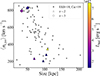 |
Fig. 1. Distribution of the Lyα nebulae around the targets in our sample in the velocity dispersion–size plane. The gray dots represent the parent sample from which our sources were selected, namely Arrigoni Battaia et al. (2019) (FAB+19) and Cai et al. (2019). Triangular and diamond markers indicate the targets selected for our study at z ∼ 2 and z ∼ 3, respectively. The points are color coded by bolometric luminosity, Lbol. |
Main properties of the six observed Type I QSOs in our sample.
2.2. Observations
2.2.1. VLT/ERIS
The ERIS (Davies et al. 2023) observations of the objects in our sample were acquired in service-mode under the ESO program 113.26AT (PI: Mainieri) at the VLT 8.2 m telescope UT4 in noAO mode. The observations were performed with the SPIFFIER IFS with a pixel scale of 250 mas/pixel, and a field of view (FoV) of 8″ × 8″, which is optimal to map the ISM regions of quasars at cosmic noon. To cover the redshifted [O III] λ5007 emission line, we used the Hlow (1.45−1.87 μm, spectral resolution of R ∼ 5200) and Klow (1.93−2.48 μm, R ∼ 5600) grating for the targets at z ∼ 2 and z ∼ 3, respectively. Individual exposures of 3600 s were obtained and repeated three times for the z ∼ 2 objects (a total of 3 h per target) and four times for the z ∼ 3 objects (a total of 4 h per target). Dithering within the ERIS FoV was applied to enable accurate sky subtraction without loss of on-source time.
2.2.2. GEMINI/GNIRS
The GNIRS observations were conducted as part of the program GN-2024A-Q-302 (PI: Farina) at Gemini North. The instrument was configured in the LR-IFU mode, which has a FoV of 3.15″ × 4.80″. We used the Short Blue camera, which provides a pixel scale of 0.15″/pixel and a grating of 32 l/mm, for a nominal spectral resolution of R∼ 1700. To cover the redshifted [O III] λ5007 emission line from the quasar, the observations were taken in the K-band. The data was collected at two position angles: PA = 0 and PA = 90, each comprising 2 × ABA′ sequences (where B indicates an empty sky location and A and A′ are two slightly dithered exposures on the source). Each exposure lasted 200 s, for a total time of 1600 s on target.
3. Data reduction
3.1. VLT/ERIS
We performed the data reduction of the targets observed with VLT/ERIS using the ESO ERIS-SPIFFIER Pipeline (v. 1.7.0), which consists of eight consecutive tasks. The first step, carried out with the eris_ifu_dark task, calculates a master dark frame and a bad pixel mask using five dark exposures taken during the observation night. Next, the task eris_ifu_detlin uses a set of one hundred and fifty flat frames taken with increasing exposure time to create a map of detector pixels with nonlinear response to input light. As the raw detector image is bent horizontally, eris_ifu_distortion performs a north-south data reduction by deriving a set of 2D polynomials using calibration frames from slit masks and arc lamps. These polynomials warp each slitlet to a rectified 64-pixel-wide image, aligning edges and straightening spectral traces.
Following, eris_ifu_flat uses ten flat frames to determine the master flat and corrects for detector responsiveness. The wavelength calibration is performed by the task eris_ifu_wavecal, which uses three arc lamps from neon, argon, and kripton to compare to a reference line list. The next step in the data reduction process uses a standard star observed right before or after the science observation. However, as this was not available, for all the targets in our sample we used the observation of the archival standard star Feige 110 in the same band, with the same pixel scale and grating, closest to the night of our science observation. We use the observation of the standard star with the task eris_ifu_stdstar to calculate the instrument response function and the flux calibration. The data cubes of the multiple science frames in an observation are created by the task eris_ifu_jitter. This task combines and applies the previously mentioned corrections to each of the raw science frames. Additionally, it performs the sky subtraction according to the Ric Davies method (Davies 2007) using the closest in time off-source sky frame.
A correction of the differential atmospheric refraction was applied at this stage to account for the effect of the stratified density structure of Earth’s atmosphere, which displaces a source by an amount dependent on the wavelength. The final step in the data reduction process corresponds to the combination of the data cubes obtained by eris_ifu_jitter for the multiple frames within a single observation, and for different observations of the same target. This step is carried out by the task eris_ifu_combine_hdrl. As the target is dithered inside the FoV, its position in each frame is different; therefore, the combination of data cubes is done based on the offset of the source in each frame, relative to its position in the first frame of the first observation. The offsets in the x and y directions are calculated by subtracting the positions of the flux centroids of two consecutive data cubes, estimated using a 2D-Gaussian fit.
We processed the final combined data cube of each target to correct for telluric absorption and performed the flux calibration using archival observations of standard stars observed at similar airmass and with the same setup as the science targets.
The end product corresponds to a flux and wavelength-calibrated, sky-corrected combined cube, with a pixel scale of 125 mas/pixel. The rest-frame optical wavelength range varies slightly for each target, but it is generally between 4600−5600 Å.
3.2. GEMINI/GNIRS
We performed the data reduction of the targets observed with GEMINI/GNIRS within the Gemini IRAF environment (Gemini Observatory & AURA 2016), adding custom made routines to improve the local sky subtraction and the alignment of the different frames. We carried out the single cube combination with the pyfu package1. The telluric absorption correction and relative flux calibration were performed using A0V stars observed at a similar airmass and in the same configuration as the science targets.
4. Data analysis
4.1. Spectra fitting
The main aim of this work is to use the [O III] λ5007 emission line to trace and characterize the presence of AGN-driven outflows in the ISM. This procedure requires spatially resolving the kinematics of the gas at kiloparsec-scales, which implies performing a spaxel-by-spaxel fit of the IFU observations to identify the [O III] λ5007 line properties across the FoV. This process was carried out in two main steps, following the approach from previous studies tracing AGN-driven outflows (Kakkad et al. 2020; Tozzi et al. 2021). First, we modeled the BLR emission using an integrated spectrum extracted from the nuclear region of the quasar. This BLR emission is unresolved in our observations; therefore, we did not expect any change in its kinematics across the FoV (see Section 4.1.1). Then, we used this BLR template to perform the spaxel-by-spaxel modeling and spatially resolve the ionized emission at ISM scales (see Section 4.1.2).
4.1.1. Modeling the unresolved emission
We start by modeling the emission from an integrated spectrum extracted from a circular aperture with a radius of one pixel, centered around the quasar centroid. On this spectrum, we restricted the wavelength range to exclude noisy channels at the edges. The spectrum was centered on the systemic velocity given by the peak of the [O III] λ5007 line. As the sky–subtraction procedure described in Section 3.1 is not optimal, we applied a sigma–clipping algorithm, rejecting flux values above 6σ and below 2σ. The clipped values were replaced using a piecewise linear interpolation method. The resulting H-band spectrum contains the doublet [O III] λ4959, 5007, a strong Hβ line, a contribution from the quasar continuum, and FeII emission (e.g., see Fig. 2). Each of the spectral components was modeled simultaneously using the lmfit package in Python. We outline the process in the following:
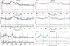 |
Fig. 2. Modeling of the integrated spectrum with an aperture of one pixel around the quasar center. Top: Total spectral profile (solid blue line) and its individual components. The orange line represents the [O III] λ4959, 5007 NLR component. The green line represents the outflowing component in the [O III] λ4959, 5007 line. The Hβ line is modeled with a broad component for the BLR shown in purple, a narrow component for the NLR shown in brown, and an additional broad component for the outflowing gas in pink. The FeII emission is shown in gray, and the linear continuum is shown in red. Bottom: Residuals of the total fit. The gray-shaded bands in both panels correspond to remnant sky emission after applying the sigma-clipping algorithm mentioned in Sect. 4.1.1. |
-
The continuum was modeled using a linear function (red line in Fig. 2).
-
Each of the components of the doublet [O III] λ4959, 5007 was modeled with two Gaussians: a narrow component (orange line in Fig. 2) and a broad component to reproduce the extended line wing(s), which point to the presence of outflows (green line in Fig. 2 ). For the narrow component of [O III] λ5007, the prior on the centroid was set to the vacuum wavelength of 5008.239 Å, with FWHM ≤ 150 km s−1. For the broad component, the centroid was restricted to the range [4900−5100 Å], and the prior on the FWHM was set to be three times higher than that of the narrow component. The centroid of the narrow and broad components of [O III] λ4959 was set to have a fixed offset of 47.94 Å from that of the narrow and broad components of [O III] λ5007, respectively. This value is estimated from the vacuum wavelength of [O III] λ4959 (4960.295 Å). The FWHM of both components of [O III] λ4959 was fixed to be equal to that of both components of [O III] λ5007, as they are expected to originate from the same gas. The ratio of the amplitudes of [O III] λ5007 to [O III] λ4959 was fixed to 2.99 for both the narrow and broad components, as demonstrated by atomic physics (Storey & Zeippen 2000; Dimitrijević et al. 2007).
-
The Hβ line was modeled using three Gaussian components: a very broad component (FWHM > 1500 km s−1) centered at the vacuum wavelength of Hβ (λ 4862.721 Å) (purple line in Fig. 2), a broad component (pink line in Fig. 2), and an additional narrow component (brown line in Fig. 2). The centroid and FWHM of the last two components of Hβ were tied to those of [O III] λ5007.
-
The FeII emission was modeled using the semi-analytic templates of Kovačević et al. (2010) (gray line in Fig. 2). We fit each of the 21 templates and chose the one that generated the fit with the minimum χ2.
After modeling and fitting the integrated spectrum with the multiple components described above, we determined the velocity centroid and FWHM of the BLR contribution to Hβ, together with the relative amplitudes of the components of the adopted Fe II template. These parameters were kept fixed during the spaxel–by–spaxel fitting, as we do not expect them to change across the FoV. This assumption is based on the spatially unresolved nature of the BLR (Hβ + Fe II), which implies that its emission scales in amplitude like the instrumental point spread function (PSF) across the FoV.
Properties of the Lyα nebulae around the QSOs in our sample.
4.1.2. Spaxel-by-spaxel fitting
We modeled the emission in each spaxel of the datacube using the same spectral components as for the integrated spectrum (Sect. 4.1.1), fixing the BLR velocity centroid and dispersion to the values derived previously and allowing only its amplitude to vary. Because the S/N varies across the FoV, applying this model uniformly may lead to overfitting in low S/N regions. To account for this, we evaluated each spaxel individually to determine the number of Gaussian components required to reproduce the [O III] doublet and Hβ emission. For this purpose, we tested two different models: Model A, identical to that used for the integrated spectrum modeling the BLR emission (Sect. 4.1.1), with two Gaussian components for each [O III] feature and three for Hβ. And Model B, a simplified version with one Gaussian component per [O III] feature and two for Hβ: a very broad component (FWHM > 1500 km s−1) tracing the emission from the BLR and a narrow component tracing the emission from the NLR.
For both models, we subtracted the contribution of all unresolved components (continuum + Hβ + [Fe II]) and that of the [O III] λ4959 line from the observed spectrum. This procedure isolates the [O III] λ5007 emission and removes blending with adjacent components. The residual spectrum obtained after subtracting Model A was fitted with two Gaussians, while that obtained after subtracting Model B was fitted with a single Gaussian.
We then computed the Bayesian Information Criterion (BIC) for both versions of the fit of the subtracted spectrum. We chose to fit the spaxel with Model A when the inclusion of additional Gaussian components provided a statistically significant improvement (i.e., when the BIC difference between the two models exceeded a target-specific threshold). Otherwise, Model B was adopted to avoid overfitting. The resulting modeled cube was visually inspected, and further manual adjustments were applied where necessary. The properties of the [O III] λ5007 emission line ([O III] hereafter) used in the subsequent analysis were derived from the preferred fit of the subtracted spectrum.
4.2. Lyα nebulae properties
The extended Lyα nebulae around the quasars in our sample were studied in a previous work by Cai et al. (2019) for targets at z ∼ 2. These observations with KCWI have a FoV of 16.8″ × 20″ and seeing in the range of 0.8″ − 1.0″. For targets at redshift z ∼ 3, the nebulae were studied by Arrigoni Battaia et al. (2019) using MUSE. These observations have a FoV constrained to the central 55″ × 55″, with seeing of 1.07″. Table 1 summarizes the instrument used to detect the extended Lyα emission around our quasars. From these studies, we used the extracted SB maps and re-analyzed them to homogeneously define the main properties of the Lyα nebulae across our sample. The Lyα SB maps are shown in Fig. 3, smoothed with a Gaussian filter of FWHM = 1″. We overlay the contours corresponding to S/N = 2, 5 and 10, i.e., each contour encloses regions where the SB lies above the 2, 5, and 10σ limit, respectively. σ corresponds to the noise level estimated in the previous studies and tabulated in Table 2.
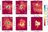 |
Fig. 3. Optimally extracted SB maps of the Lyα nebulae surrounding the quasars (see Sect. 4.2). The white, gray, and black contours represent 2σ, 5σ, and 10σ, respectively. The values of σ are reported in Table 2. The green cross in the center represents the position of the quasar, determined by estimating the photocentroid of a channel map in a wavelength where the Lyα line is not present. North is up; east is left. |
We characterized the Lyα nebulae using the S/N > 2 isophote. For each source, we measure the area enclosed by this contour and define DLyα as the diameter of a circle with the same area, which we adopt as our size estimator. Size uncertainties are dominated by calibration errors, which we assume as 5% Bacon et al. (2010). Therefore, we constrain the Lyα nebulae size by measuring the S/N > 1.9 and S/N > 2.1 isophotes, which we quote as the upper and lower bounds, respectively.
The Lyα luminosity, LLyα, is obtained by integrating the SB within the S/N > 2 contour. In some cases, this isophote extends beyond the FoV, and therefore, the sizes and luminosities correspond to lower limits. The luminosity uncertainty is estimated as ΔLLyα = σbkg ⋅ Apix ⋅ Npix, where σbkg is the standard deviation of the SB in source–free regions, Apix is the pixel area, and Npix is the number of pixels enclosed by the S/N > 2 contour. The resulting measurements are listed in Table 2.
Following the approach by Arrigoni Battaia et al. (2019), we used 30 Å narrow-band images to derive the SB radial profiles of the nebulae, shown in Fig. 4. To do this, we created a grid of radial distances of every pixel from the quasar center, considering the rectangular pixel scale. Based on this, we defined bins (annuli) of the same radial distance and estimated the mean SB for each bin. The gray line in Fig. 4 shows  , corresponding to the 2σ detection limit estimated for each annulus. This value was estimated as
  , where Aannulus corresponds to the area of the annulus and SBarcsec2lim corresponds to the SB limit per arcsec2. The latter was estimated as
  , where Apix corresponds to the pixel area and SBpix to the SB uncertainty per pixel. The SB uncertainty per pixel was calculated as the rms noise of out-of-source regions. For the extraction of the SB profiles, we masked the central source region, defined as a circle of radius 0.5 arcsec2, since this was used as a normalization region to subtract the quasar PSF and is affected by residuals. The profile is plotted up to the size of the nebula estimated using the S/N > 2 isophote.
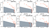 |
Fig. 4. Lyman-α SB radial profiles. The red points show the average SB per radial annulus, while the gray line denotes the 2σ detection limit estimated for each annulus. |
5. Results
5.1. Spatially resolved and extended emission
After modeling the [O III] line emission across the FoV following our spectral fitting procedure (Sect. 4.1.2), it is necessary to establish whether the observed emission is truly extended and spatially resolved, rather than being dominated by instrumental PSF or beam-smearing effects. Following the approach of Kakkad et al. (2020), we conducted two independent tests to address this question.
The first test consists of comparing the curve of growth (COG; i.e., the flux within circular apertures as a function of radius, centered on the AGN) of the [O III] emission with that of the PSF, to search for significant excess emission. As no dedicated standard-star observation is available, we used the unresolved point-like BLR emission as a proxy for the PSF. To construct the COGs of both the [O III] and BLR emission, we first created their flux maps based on the spaxel-by-spaxel modeling described in Sect. 4.1.2. Using such maps, we measured the mean flux in concentric circular apertures spanning radii from two to ten kiloparsecs in one-kiloparsec steps, and subsequently normalized by the flux in the innermost aperture. The resulting COGs are presented in Fig. 5, where the [O III] emission is shown in blue and the BLR-PSF in red.
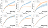 |
Fig. 5. Curve of growth of the [O III] (blue) and BLR normalized flux (red) in log scale. Targets Q0050+0051, Q0052+0140, and SDSSJ2319-1040 show evidence of spatially resolved [O III] emission. |
Figure 5 shows that the [O III] emission in Q0050+0051, Q0052+0140, and SDSSJ2319−1040 is spatially resolved, as its normalized flux increases more rapidly with the radius than that of the PSF. In contrast, the COG of the [O III] emission in Q2121+0052 remains below that of the PSF at all radii, indicating that the emission is not resolved. For Q2123−0050 and SDSSJ1427−0029, the normalized [O III] and BLR fluxes grow at a similar rate across all radii, suggesting that the emission is unresolved as well.
For the second test, we followed the PSF-subtraction method described in Husemann et al. (2016) and Kakkad et al. (2020) to identify the presence of extended emission. We first extracted the nuclear spectrum from an aperture of one pixel around the quasar. This spectrum was fitted with a model f(x), identical to the one described in Sect. 4.1.1. The rest of the pixels were fitted with a model f′=a * f(x), where a corresponds to the rescaling factor. This model f′, accounting for the contribution from the PSF, was subtracted from the observed spectrum in each pixel. After such subtraction, any remnant [O III] emission is considered to be extended and not BLR-dominated as a consequence of beam smearing from the PSF. To map such emission, we created narrow median maps (between 5–15 Å wide) around the center of the [O III] line. The results are shown in Fig. 6. We observe that four targets show signs of extended [O III] emission. Three of these targets, namely Q0050+0051, Q0052+0140, and SDSSJ2319−1040, had previously been identified to be spatially resolved in the first test carried out from Fig. 5. Although Q2123−0050 had previously shown unresolved emission, Fig. 6 shows the presence of extended emission above the 2σ level. We can then conclude that any [O III] emission detected by the spaxel-by-spaxel fitting from these four targets is extended and/or spatially resolved, and we can rely on the kinematic maps described in Sect. 5.2 to characterize the extension and morphology of the ionized outflows. In contrast, Q2121+0052 and SDSSJ1427−0029 show no evidence of extended [O III] emission. As these targets fail to show resolved and/or extended emission in both tests, we refrain from performing the spatially resolved analysis for them.
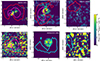 |
Fig. 6. Median maps of the residual [O III] emission after PSF subtraction. Targets Q0050+0051, Q0052+0140, Q2123-0050, and SDSSJ2319-1040 show evidence of extended [O III] emission. The magenta, red, and cyan contours represent 5σ, 10σ, and 30σ contours of the Lyα SB maps, respectively. The white cross represents the AGN center. North is up; east is left. |
5.2. Ionized gas kinematics
We characterized the [O III] line by measuring the velocity at the 10th, 50th, and 90th percentile (v10, v50, and v90, respectively). The extreme velocities v10 and v90 are representative of the blue and red-shifted emission in the wings of the line, respectively. The velocity width is measured by w80, which contains 80% of the total line flux (w80 = v90 − v10). The values of v10, v90, and especially w80 are widely used in the literature to test the presence of fast outflowing gas (e.g., Liu et al. 2013; Harrison et al. 2016; Temple et al. 2019; Kakkad et al. 2020; Tozzi et al. 2024).
Figure 7 shows the [O III] total flux and velocity maps for the targets in the sample with spatially resolved and/or extended emission, as demonstrated in Sect. 5.1. The [O III] total flux corresponds to the flux of the sum of the Gaussian components used to model the line. The second, third and fourth column show the velocities v10, v90 and the width w80 respectively. The cross marks the position of the AGN center, which we determined by estimating the photo-centroid of the flux map at 5100 Å. At this wavelength, the emission is dominated only by the AGN continuum, and therefore it is a good tracer for the emission close to the supermassive BH. The kinematics maps were created by excluding pixels with S/N < 2.
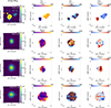 |
Fig. 7. Flux and kinematics maps of the [O III] emission for the targets showing spatially resolved and/or extended emission. The first column shows the flux map of the [O III] emission. The second, third, and fourth columns show the v10, v90, and w80 velocity maps, respectively. The black cross marks the AGN center. North is up; east is left. |
5.3. Outflow detection
The kinematics of the NLR is typically traced by relatively narrow systemic Gaussian components. In the presence of AGN-driven outflows, however, the [O III] line profile becomes asymmetric, showing extended wings that require additional broad Gaussian components to accurately reproduce the spectrum. The resulting asymmetry of the [O III] line profile is indicative of outflowing ionized gas, which translates into extreme velocity values. As discussed in Sect. 5.2, different studies have adopted various definitions of outflow velocity based on different parameters. In this work, we adopt the nonparametric line width w80 as our tracer of the ionized gas velocity. Compared to v10 or v90, w80 is less sensitive to projection effects (e.g., due to galaxy inclination; Harrison et al. 2012), although it may be more affected by dust extinction (Tozzi et al. 2024). In our case, this effect is negligible, as our sample consists of bright Type I QSOs where obscuration is expected to be minimal.
We used the w80 maps presented in the fourth column of Fig. 7 to investigate the presence of AGN-driven outflows in our sample. The ionized gas in a given spaxel is classified as part of an outflow when w80 ≥ 600 km s−1 (e.g., Harrison et al. 2012, 2016; Kakkad et al. 2016, 2020). This threshold is deliberately conservative: numerical experiments of AGN winds interacting with a clumpy ISM show that outflowing gas can exhibit considerably lower bulk velocities, down to ∼100 km s−1, while still being distinguishable from the effect of the host-galaxy kinematics (Ward et al. 2024). In observations, however, decoupling the low-velocity outflowing component from the host’s contribution is not straightforward. Therefore, we limit our analysis to the gas that can be unambiguously classified as outflowing material, i.e., that with w80 ≥ 600 km s−1.
Following our definition, all spatially resolved targets in our sample show evidence for AGN-driven outflows. In Q0050+0051, we identify an [O III] emission region northwest of the source; however, this structure is distinct from the main outflow, where gas velocities exceed 2000 km s−1 (see Sect. 6.2 for further discussion). For the remaining three resolved sources, we measure ionized gas velocities of at least 1100 km s−1, consistent with gas moving significantly faster than the systemic velocity of the host galaxy. Regions of high w80 show a mild spatial gradient in Q0051+0140 and Q2123−0050, while they appear more spherically symmetric in Q0050+0051 and SDSSJ2319−1040. A comparison with the v10 maps (first column of Fig. 7) shows that the w80 peaks coincide with the highest velocity shifts (v10 < −1000 km s−1), indicating the presence of a strongly blueshifted component. Similarly, the v90 maps (second column of Fig. 7) reveal milder redshifted components (up to ∼1270 km s−1) coincide spatially with the w80 and v10 peaks. This configuration is consistent with a biconical outflow geometry, where the approaching (blueshifted) side is visible, while the receding (redshifted) counterpart is likely obscured by dust in the galactic disk.
Alternative scenarios such as SF-driven outflows, inflows, mergers, or turbulence are unlikely to explain the observed high-velocity dispersions and velocity shifts, as well as the asymmetric line profiles. SF-driven outflows and inflows typically exhibit much lower velocities of ∼500 km s−1 (Arribas et al. 2014; Schreiber et al. 2019) and ∼200 km s−1 (Bouché et al. 2013; Liu et al. 2025), respectively, with the latter usually detected in absorption. In contrast, merger-driven kinematics would produce symmetric double-peaked line profiles rather than the asymmetric blueshifted components observed here.
After successfully detecting outflows in the resolved targets of our sample, we estimated their extension and velocity, which are needed to determine the outflow energetics. We used the kinematics maps in Fig. 7 to estimate these values. The extension of the outflow, Rout, is defined as the largest distance between the ionized gas and the AGN center. The velocity of the outflow, vout, is defined as the maximum value observed in the w80 map, assuming the outflow has a constant velocity, and therefore any smaller velocities are produced by projection effects.
We define the outflow luminosity, ![Mathematical equation: $ L_{\mathrm{out}}^{[\mathrm{OIII}]} $](/articles/aa/full_html/2026/03/aa57861-25/aa57861-25-eq10.gif) , as the luminosity estimated from the flux contained in the high-velocity channels (v ≥ 300 km s−1, Kakkad et al. 2020) of all spaxels with S/N > 2. The estimated values of extension, velocity, and luminosity of the AGN-driven outflows in our sample are shown in the second, third, and fourth column of Table 3, respectively.
, as the luminosity estimated from the flux contained in the high-velocity channels (v ≥ 300 km s−1, Kakkad et al. 2020) of all spaxels with S/N > 2. The estimated values of extension, velocity, and luminosity of the AGN-driven outflows in our sample are shown in the second, third, and fourth column of Table 3, respectively.
Properties of the [O III] ionized outflows.
For the unresolved targets Q2121+0052 and SDSSJ1427−0029, we are limited by the PSF to perform any spatial analysis on the ionized gas. However, we can still detect the presence of AGN-driven outflows by analyzing the [O III] line profile extracted from an integrated spectrum centered around the quasar. The aperture of this spectrum was set to 0.25″ for Q2121+0052 (see Fig. A.1) and 0.75″ for SDSSJ1427−0029 (see Fig. A.2), corresponding to roughly 2 kpc and 6 kpc, respectively. These values were determined by creating a channel map around the location of the [O III] line, and determining the radius where 99.5% of the flux is contained. From this integrated spectrum, we observed an asymmetric [O III] profile, which we modeled as described in Sect. 4.1. The nonparametric analysis of the line profile indicates ionized gas w80 velocities consistent with our definition of AGN-driven outflows. We estimate the properties of this outflow in the same way as for the spatially resolved sources, with the difference that the resulting values on the extension, velocity and luminossity of the outflow correspond only to upper limits.
The fitting uncertainties on vout and ![Mathematical equation: $ L_{\mathrm{out}}^{[\mathrm{OIII}]} $](/articles/aa/full_html/2026/03/aa57861-25/aa57861-25-eq13.gif) are estimated as follows. We extract an integrated spectrum containing roughly 95% of the total [O III] flux of the quasar. By adding rms noise to the best fit of this spectrum, we created 100 mock spectra and fit each of them using the procedure mentioned in Sect. 4.1.1. The errors reported in Table 3 correspond to the 1σ uncertainties resulting from these iterations. Considering the resolving power of VLT/ERIS and GEMINI/GNIRS, the uncertainty on w80 due to the instrumental resolution is expected to be negligible compared to the fitting uncertainty. Although we do not have an accurate estimate on the uncertainties of Rout, we do not expect them to be smaller than the pixel scale of the observations with VLT/ERIS, corresponding to 0.125″/pix.
are estimated as follows. We extract an integrated spectrum containing roughly 95% of the total [O III] flux of the quasar. By adding rms noise to the best fit of this spectrum, we created 100 mock spectra and fit each of them using the procedure mentioned in Sect. 4.1.1. The errors reported in Table 3 correspond to the 1σ uncertainties resulting from these iterations. Considering the resolving power of VLT/ERIS and GEMINI/GNIRS, the uncertainty on w80 due to the instrumental resolution is expected to be negligible compared to the fitting uncertainty. Although we do not have an accurate estimate on the uncertainties of Rout, we do not expect them to be smaller than the pixel scale of the observations with VLT/ERIS, corresponding to 0.125″/pix.
5.4. Outflow energetics
The outflow energetics can be derived using the outflow extension, velocity, and luminosity (Rout, vout, and ![Mathematical equation: $ L_{\mathrm{out}}^{[\mathrm{OIII}]} $](/articles/aa/full_html/2026/03/aa57861-25/aa57861-25-eq14.gif) ) estimated in the previous section. The outflow mass Mout can be estimated as follows (e.g., Carniani et al. 2015; Kakkad et al. 2020; Tozzi et al. 2024):
) estimated in the previous section. The outflow mass Mout can be estimated as follows (e.g., Carniani et al. 2015; Kakkad et al. 2020; Tozzi et al. 2024):
![Mathematical equation: $$ \begin{aligned} M_\mathrm{out} ^{\mathrm{[OIII]} } = 0.8 \times 10^8\, \mathrm{M} _\odot \left( \frac{L_{\mathrm{out} }^{[\mathrm{OIII} ]}}{10^{44}\,\mathrm {erg\,s}^{-1} } \right)&\left( \frac{n_\mathrm{e} }{500\,\mathrm {cm}^{-3} } \right)^{-1} \nonumber \\&\left( \frac{1}{10^{\mathrm{[O/H]} - \mathrm{[O/H]} _\odot }} \right), \end{aligned} $$](/articles/aa/full_html/2026/03/aa57861-25/aa57861-25-eq15.gif) (1)
(1)
where all oxygen is assumed to be ionized to O2+, the electron temperature is taken to be T ∼ 104 K, ne denotes the electron density, and [O/H] represents the oxygen abundance, assumed to be solar. The electron density is commonly inferred from the [S II]λ6716/[S II] λ6731 flux ratio; however, our observations do not cover such emission lines. In the literature, the electron density ne spans several orders of magnitude, typically ranging from 102 to 104 cm−3 (e.g., Cano-Díaz et al. 2012; Fiore et al. 2017; Perna et al. 2017; Baron & Netzer 2019). We adopt a fiducial value of ne = 500 ± 250 cm−3, consistent with previous studies and with measurements reported for AGN at z ∼ 2 (Harrison et al. 2014; Cresci et al. 2023; Tozzi et al. 2024). As demonstrated by Kakkad et al. (2020), this uncertainty in ne alone can result in variations of up to an order of magnitude in the inferred outflow mass rate. Consequently, the adopted value of ne constitutes the dominant source of uncertainty in our estimates of the outflow energetics.
The outflow mass rate depends on the outflow geometry. For an outflow with a bi-conical or spherical geometry, filled with uniformly distributed clouds of the same density and constant outflow velocity, the outflow mass rate and outflow kinetic power are independent of the outflow opening angle and the filling factor of the clouds in the cone (Husemann et al. 2016).
In this scenario, the outflow mass rate, corresponding to the instantaneous outflow mass rate of ionized gas crossing the spherical sector at a distance Rout from the AGN, can be estimated as
![Mathematical equation: $$ \begin{aligned} \dot{M}_\mathrm{out} ^{\mathrm{[OIII]} } = 3 \frac{M_\mathrm{out} ^{\mathrm{[OIII]} }\ v_{\mathrm{out} }}{R_{\mathrm{out} }}\cdot \end{aligned} $$](/articles/aa/full_html/2026/03/aa57861-25/aa57861-25-eq16.gif) (2)
(2)
For an outflow propagating in thin shells of thickness ΔR that shock against the ISM, the localized outflow mass rate at the shell distance from the nucleus is independent of the outflow opening angle, and it can be estimated as
![Mathematical equation: $$ \begin{aligned} \dot{M}_\mathrm{out} ^{\mathrm{[OIII]} } = \frac{M_\mathrm{out} ^{\mathrm{[OIII]} }\ v_{\mathrm{out} }}{\Delta R}\cdot \end{aligned} $$](/articles/aa/full_html/2026/03/aa57861-25/aa57861-25-eq17.gif) (3)
(3)
In this work, we adopt the simplified bi-conical or spherical outflow geometry described by Equation (2). This choice is conservative, as a shell-like geometry yields higher estimates of the outflow mass rate (Maiolino et al. 2012; Husemann et al. 2019; Kakkad et al. 2020), while our data lacks the spatial resolution required to constrain the shell thickness in such a scenario. Additionally, as discussed in Cicone et al. (2014), a bi-conical or spherical geometry provides a physically motivated description of feedback scenarios in which the outflow is continuously replenished by clouds ejected from the galactic disk.
The outflow kinetic power was estimated as
![Mathematical equation: $$ \begin{aligned} \dot{E}_\mathrm{kin} ^{\mathrm{[OIII]} } = \frac{3}{2} \frac{M_\mathrm{out} ^{\mathrm{[OIII]} }\ v_{\mathrm{out} }^3}{R_{\mathrm{out} }}\cdot \end{aligned} $$](/articles/aa/full_html/2026/03/aa57861-25/aa57861-25-eq18.gif) (4)
(4)
The values of the ionized outflow energetics are reported in Table 3. The associated uncertainties were estimated by error propagation. As discussed in Sect. 5.3, we adopted a conservative velocity threshold of w80 ≥ 600 km s−1 to identify outflowing gas, implying that only the high-velocity component is considered in the estimation of the outflow energetics. Consequently, the derived ionized outflow mass should be interpreted as a lower limit, since a significant fraction of the mass is expected to move at lower velocities (Costa et al. 2018). The effect of this threshold on the kinetic energy is, however, negligible, as the bulk of the power originates from the high-velocity gas (Ward et al. 2024).
6. Discussion
As shown in Sect. 5.3, for all the quasars with known Ly α nebulae that we have observed with VLT/ERIS and GEMINI/GNIRS, we have detected the presence of galaxy-wide AGN-driven outflows. These outflows are much more luminous and have a higher kinetic power than those detected in previous studies (Kakkad et al. 2020; Tozzi et al. 2024). While this is interesting, it is not clear proof of a causal connection between the two phenomena. To investigate how the detected outflows may be connected to the extended Lyα nebulae surrounding the quasar, we now focus on exploring the correlation between different physical parameters of both phenomena.
6.1. Outflow kinetic power versus Lyα nebulae size and luminosity
Costa et al. (2022) find that the size and luminosity of the nebulae are set by the escape of Lyα and ionizing flux from the galactic nucleus. The more the gaseous reservoir in the nucleus is cleared out, the higher the escape fraction. We may thus expect a connection between the outflow kinetic power and the physical properties of the Lyα nebula.
An increasingly powerful outflow may directly (e.g., by recombination in photoionized regions) or indirectly (e.g., by opening a path of low optical depth for the Lyα and UV photons from the BLR to escape) contribute to further ionize the CGM and generate Lyα nebulae on larger scales. To test this prediction, we compare the kinetic power of the AGN-driven outflows detected in the quasars presented in this work, with the size (see Fig. 8) and luminosity (see Fig. 9) of their corresponding Lyα nebulae.
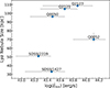 |
Fig. 8. Relation between outflow kinetic power and Lyα nebulae size. |
Figures 8 and 9 suggest that both the size and luminosity of the Lyα nebulae may increase with the kinetic power of the AGN-driven outflows traced on ISM scales. To quantify the strength of these possible relations, we computed the Pearson correlation coefficients. For the relation between outflow power and Lyα nebula size (![Mathematical equation: $ \dot{E}_{\mathrm{kin}}^{\mathrm{[OIII]}} $](/articles/aa/full_html/2026/03/aa57861-25/aa57861-25-eq19.gif) –DLyα), we find r = 0.39 with a null-hypothesis probability of ∼43%. For the relation between outflow power and Lyα nebula luminosity (
–DLyα), we find r = 0.39 with a null-hypothesis probability of ∼43%. For the relation between outflow power and Lyα nebula luminosity (![Mathematical equation: $ \dot{E}_{\mathrm{kin}}^{\mathrm{[OIII]}} $](/articles/aa/full_html/2026/03/aa57861-25/aa57861-25-eq20.gif) –LLyα), we obtain r = −0.01 with a null-hypothesis probability of ∼98%. These results indicate very weak and statistically nonsignificant linear correlations between the outflow power and the Lyα nebulae properties. However, considering that these relations may not be strictly linear, a Spearman rank correlation test would provide a more appropriate measure of any monotonic trend. The use of this nonparametric test is further motivated by the presence and effect of potential outliers. As shown in Figs. 8 and 9, Q0052+0140 deviates from the overall trends: despite exhibiting relatively high [O III] outflow kinetic power and luminosity, it is not associated with a comparably extended or luminous Lyα nebula. We propose two plausible explanations for this discrepancy. The first is related to orientation and scattering effects. In particular, the Lyα nebula in Q0052+0140 appears one-sided. As discussed by Costa et al. (2022), the escape of Lyα photons from the nuclear regions is highly anisotropic due to the combined effects of dust absorption and resonant scattering. Lyα photons preferentially escape along the galaxy’s rotation axis, such that lines of sight intersecting the disk plane are expected to produce fainter and more asymmetric nebulae than face-on orientations. The second explanation involves the impact of an over-efficient AGN-driven outflow. The outflow detected in Q0052+0140 exhibits the highest kinetic power of our sample of quasars. Costa et al. (2022) shows that when the wind kinetic power exceeds the level required to simply open a low-optical-depth channel, it removes most of the neutral hydrogen from the inner halo. In this regime, Lyα photons escape directly from the nucleus rather than being resonantly scattered through the CGM, resulting in a compact and faint Lyα nebula.
–LLyα), we obtain r = −0.01 with a null-hypothesis probability of ∼98%. These results indicate very weak and statistically nonsignificant linear correlations between the outflow power and the Lyα nebulae properties. However, considering that these relations may not be strictly linear, a Spearman rank correlation test would provide a more appropriate measure of any monotonic trend. The use of this nonparametric test is further motivated by the presence and effect of potential outliers. As shown in Figs. 8 and 9, Q0052+0140 deviates from the overall trends: despite exhibiting relatively high [O III] outflow kinetic power and luminosity, it is not associated with a comparably extended or luminous Lyα nebula. We propose two plausible explanations for this discrepancy. The first is related to orientation and scattering effects. In particular, the Lyα nebula in Q0052+0140 appears one-sided. As discussed by Costa et al. (2022), the escape of Lyα photons from the nuclear regions is highly anisotropic due to the combined effects of dust absorption and resonant scattering. Lyα photons preferentially escape along the galaxy’s rotation axis, such that lines of sight intersecting the disk plane are expected to produce fainter and more asymmetric nebulae than face-on orientations. The second explanation involves the impact of an over-efficient AGN-driven outflow. The outflow detected in Q0052+0140 exhibits the highest kinetic power of our sample of quasars. Costa et al. (2022) shows that when the wind kinetic power exceeds the level required to simply open a low-optical-depth channel, it removes most of the neutral hydrogen from the inner halo. In this regime, Lyα photons escape directly from the nucleus rather than being resonantly scattered through the CGM, resulting in a compact and faint Lyα nebula.
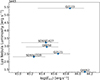 |
Fig. 9. Relation between outflow kinetic power and Lyα nebulae luminosity. |
To assess the impact of individual data points in the results of the test, we performed multiple iterations of the Spearman rank correlation test, each time excluding one source from the sample. The results are shown in Table 4.
The results of the correlation analysis presented in Table 4 indicate that excluding Q0052+0140, identified as an outlier, yields a stronger positive monotonic relation between the outflow and the Lyα nebula properties, compared to the results obtained when including all sources in the correlation test. In this case, the ![Mathematical equation: $ \dot{E}_{\mathrm{kin}}^{\mathrm{[OIII]}} $](/articles/aa/full_html/2026/03/aa57861-25/aa57861-25-eq23.gif) –DLyα relation shows a Spearman coefficient of ρ = 0.89 with a null-hypothesis probability of 3%, while the
–DLyα relation shows a Spearman coefficient of ρ = 0.89 with a null-hypothesis probability of 3%, while the ![Mathematical equation: $ \dot{E}_{\mathrm{kin}}^{\mathrm{[OIII]}} $](/articles/aa/full_html/2026/03/aa57861-25/aa57861-25-eq24.gif) –LLyα relation gives ρ = 0.6 with a null-hypothesis probability of 28%. Excluding any other source does not produce a significant change in the results.
–LLyα relation gives ρ = 0.6 with a null-hypothesis probability of 28%. Excluding any other source does not produce a significant change in the results.
These findings suggest a strong positive correlation between the outflow kinetic power and the Lyα nebula size, and a weaker correlation with the Lyα luminosity. However, given the small sample size and the limited range in Lbol and ![Mathematical equation: $ \dot{E}_{\mathrm{kin}}^{\mathrm{[OIII]}} $](/articles/aa/full_html/2026/03/aa57861-25/aa57861-25-eq25.gif) (less than one order of magnitude), a larger dataset would be required to confirm these trends more robustly.
(less than one order of magnitude), a larger dataset would be required to confirm these trends more robustly.
Both the outflow power (e.g., Fiore et al. 2017; Liu et al. 2009; Zakamska et al. 2016) and the Lyα nebula size and luminosity (e.g., Lobos et al. 2025; Mackenzie et al. 2021) are known to correlate positively with the quasar Lbol. This raises the possibility that the observed relation between outflow kinetic power and Lyα nebula properties may be indirectly driven by their mutual dependence on Lbol. To assess this, we performed a partial correlation analysis for the ![Mathematical equation: $ \dot{E}_{\mathrm{kin}}^{\mathrm{[OIII]}} $](/articles/aa/full_html/2026/03/aa57861-25/aa57861-25-eq26.gif) –DLyα and
–DLyα and ![Mathematical equation: $ \dot{E}_{\mathrm{kin}}^{\mathrm{[OIII]}} $](/articles/aa/full_html/2026/03/aa57861-25/aa57861-25-eq27.gif) –LLyα relations while controlling for Lbol. Using the simplified recursive expression for a single control variable2, we computed the corresponding partial Spearman correlation coefficients. We find ρ = 0.90 for
–LLyα relations while controlling for Lbol. Using the simplified recursive expression for a single control variable2, we computed the corresponding partial Spearman correlation coefficients. We find ρ = 0.90 for ![Mathematical equation: $ \dot{E}_{\mathrm{kin}}^{\mathrm{[OIII]}} $](/articles/aa/full_html/2026/03/aa57861-25/aa57861-25-eq28.gif) –DLyα and ρ = 0.61 for
–DLyα and ρ = 0.61 for ![Mathematical equation: $ \dot{E}_{\mathrm{kin}}^{\mathrm{[OIII]}} $](/articles/aa/full_html/2026/03/aa57861-25/aa57861-25-eq29.gif) –LLyα. These results confirm that the positive monotonic correlations between outflow kinetic power and Lyα nebula properties persist independently of Lbol and are therefore not driven by their shared dependence on AGN luminosity.
–LLyα. These results confirm that the positive monotonic correlations between outflow kinetic power and Lyα nebula properties persist independently of Lbol and are therefore not driven by their shared dependence on AGN luminosity.
6.2. Spatial relation between extended [O III] emission and Lyα nebulae
If the AGN-driven outflows on ISM scales are opening a path of least resistance for the quasar’s Lyα and UV photons to escape to the CGM, one would expect that, at such scales (inner CGM), the morphology of the Lyα nebulae is correlated with the orientation of the outflow. To investigate any possible spatial alignment between the ionization cone and the direction of the Lyα nebulae, we compare the location of the extended [O III] emission with that of the brightest regions of the nebula, represented by the highest S/N contours, S/N = 5, 10, 30.
We performed the alignment between the remnant [O III] emission and the Lyα nebulae contours by placing both datasets onto a common astrometric reference frame using the World Coordinate System information from the data cubes. We converted the pixel coordinates into projected angular offsets relative to the quasar position, and both maps were recentered such that the quasar lies at position (0,0). The Lyα SB contours were then overplotted on the [O III] extended emission maps using these common angular coordinates. This alignment is therefore based on the morphological correspondence between the two tracers, rather than on explicit position-angle measurements. The results are shown in Fig. 6.
For Q0050+0051, we detect extended [O III] emission toward the south and northwest, with the latter spatially coinciding with the peak of the Lyα SB map (Fig. 3). However, the w80 map (Fig. 7) shows that this region exhibits low velocities, inconsistent with ionized outflows. Additionally, the v50 map (Fig. 10) shows a pronounced velocity offset (Δv50 ∼ 1200 km s−1) between the central and the extended emission. Such velocity offset exceeds the typical range expected from disk rotation in star-forming galaxies at z ∼ 2 (tens to a few hundred km s−1) (e.g., Yue et al. 2021; Roman-Oliveira et al. 2023). These results suggest that the [O III] emission cloud detected toward the northwest of Q0050+0051 likely traces dynamically quiescent gas outside the main host. Nonetheless, this interpretation does not exclude the possibility of a spatial alignment between the outflow and the nebula in this source. Given that the outflow is detected only on small scales and its direction cannot be constrained with our data, we cannot rule out the scenario in which the cloud is being ionized by the AGN. In that case, the [O III] cloud might be indicating the direction of the ionization cone, likely corresponding to the direction of the inner outflow clearing the central regions.
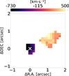 |
Fig. 10. Velocity map, v50, of Q0050+0051. |
For Q0052+0140, we detect extended [O III] emission toward the west and southeast, coincident with regions of increased w80 velocities (see Fig. 7). Notably, the Lyα nebula is also particularly bright in these directions, suggesting a possible connection between the two phenomena. In the cases of Q2123−0050 and SDSSJ2319−1040, the [O III] emission appears symmetrically extended around the quasar, which is comparable with the symmetric morphology of their Lyα nebulae (see Fig. 3).
Overall, the observed alignment between the extended O III emission and the regions of increased Lyα emission on small scales supports the scenario of a casual link between the two phenomena, with the caveat that this conclusion is based on our limited sample size.
6.3. Alternative powering mechanisms of the Lyα nebulae
The Lyα emission detected around high-redshift quasars is generally attributed to a combination of mechanisms, including recombination, gravitational cooling, and scattering of BLR photons. However, as demonstrated by Costa et al. (2022), these processes alone are insufficient to reproduce the observed bright and extended Lyα nebulae without the inclusion of AGN-driven outflows. In particular, considering BLR scattering as the only source of Lyα photons results in emission confined to the central ∼0.5 kpc, preventing the formation of an extended nebula. Conversely, considering only recombination and collisional excitation yields nebulae with larger spatial extents, but they are fainter, morphologically irregular, and not centered around the quasar.
Inspecting the Lyα SB maps of our sample (Fig. 3), we find that the nebulae associated with Q2121+0052 and SDSSJ2319−1040 closely resemble the recombination + collisional excitation scenario. These nebulae are fainter than those of the rest of the sample, and in the case of Q2121+0052, the emission is offset from the quasar location. Notably, Q2121+0052 also hosts the least extended and least luminous outflow in the sample, with the lowest outflowing mass, although its kinetic power lies within the typical range. In contrast, SDSSJ2319−1040 exhibits a widely extended but low-velocity outflow, corresponding to the lowest kinetic power among the sample. In light of the positive correlation between outflow kinetic power and Lyα nebula luminosity identified in Section 6.1, these results suggest that AGN-driven outflows play a reduced role in powering the extended Lyα emission in these two systems. Instead, consistent with the scenario proposed by Costa et al. (2022), their Lyα nebulae are likely produced by recombination with an increasing contribution from collisional excitation toward their outskirt.
To test this scenario quantitatively, we follow the approach by Hennawi & Prochaska (2013), used in the literature (e.g., Battaia et al. 2015; Farina et al. 2019; Lobos et al. 2025) to predict the SB of the Lyα emission originated from photoionization of cold gas by the AGN radiation, followed by recombination. For this purpose, we assume that quasars are surrounded by spherical gas clouds that are either optically thick ( ) or optically thin (
 ) to the Lyman continuum photons. We derive the H I column density of a single cloud as
 (5)
(5)
where LLyα represents the observed luminosity of the Lyα nebulae and LνLL is the luminosity of the quasar at the Lyman edge. The latter can be estimated assuming that the spectral energy distribution (SED) of the quasar follows a power law of the form Lν = LνLL(ν/νLL)αUV, where Lν represents the ionizing luminosity, and αUV = −0.61, following Lusso et al. (2015). For SDSSJ2319−1040,  (Allen et al. 2011), and therefore
  . In the same way for Q2121+0052,
  (Allen et al. 2011) and LνLL = 2.23 × 1031 erg s−1 Hz−1. Using the values for the quasar luminosity at the Lyman edge and those for the nebula luminosity reported in Table 2 in Equation (5), we estimate that
  and
and  for SDSSJ2319−1040 and Q2121+0052, respectively. These results are consistent with the optically thin scenario for which
 (6)
(6)
where we assume typical values of fC = 0.5 for the covering fraction of the optically thin clouds, nH = 1 cm−3 for the cloud’s hydrogen volume, and NH = 1020.5 cm−2 for its column density (e.g., Prochaska et al. 2013; Lau et al. 2016). In this regime, the expected SB does not depend on the luminosity of the quasar but only on the physical properties of the gas. Therefore, we estimate that the AGN photoionization alone will power a Lyα nebulae with SB ∼ 3.2 × 10¹⁸ erg s−1 cm−2 arcsec−2 and SB ∼ 7.4 × 10¹⁸ erg s−1 cm−2 arcsec−2, corresponding to nebula luminosities of LLyα ∼ 9 × 1042 erg s−1 and LLyα ∼ 4 × 1043 erg s−1 for SDSSJ2319−1040 and Q2121+0052, respectively. These results are consistent with the observed Lyα nebulae luminosities reported in Table 2. Hence, we can conclude that the AGN radiation provides sufficient energy to photoionize the surrounding gas and power extended but faint nebulae such as the ones observed around the quasars SDSSJ2319−1040 and Q2121+0052, with a minor contribution from AGN-driven outflows.
In addition to assessing the role of alternative mechanisms in powering the Lyα nebulae, we also examine the impact of outflow timescales. We characterize the AGN-driven outflows by estimating their dynamical ages using the velocities and extents reported in Table 3. The resulting outflow age estimates are presented in Table 5.
Outflow ages.
Assuming an AGN duty cycle of ∼1 Myr (e.g., Clavijo-Bohórquez et al. 2023; Harrison & Ramos Almeida 2024), defined as the timescale over which the supermassive BH alternates between active and inactive phases, the outflow timescales reported in Table 5 suggest that all sources in our sample, except Q2121+0052, were likely launched during previous AGN episodes. In contrast, Q2121+0052 hosts the youngest outflow, which allows us to consider a scenario in which the outflow was only recently triggered and has not yet had sufficient time to propagate through the host galaxy. As a result, its impact on increasing the escape fraction of Lyα photons from the nuclear regions may still be limited. Additionally, we find that all outflows are younger than 5 Myr, which, according to Costa et al. (2020), is sufficient time for them to propagate to scales below 10 kpc. This suggests that the observed Lyα nebulae may be the result of the cumulative effect of AGN events over the lifetime of the host galaxy, rather than due to a single episode. However, as the ionizing photons can travel faster than the outflow itself, the Lyα emission on large scales might be the result of photoionization followed by recombination processes.
7. Summary and conclusions
We have presented VLT/ERIS and GEMINI/GNIRS observations of six quasars previously known to host extended Lyα nebulae (Arrigoni Battaia et al. 2019; Cai et al. 2019) identified with VLT/MUSE and Keck/KCWI. Using near-infrared IFU data, we traced the kinematics of the ISM through the [O III] emission line (Sect. 5.2). The main results of our work are as follows:
-
We detect ionized outflows in all the targets of our sample with velocities of vout > 1500 km s−1. By comparing the [O III] and PSF-BLR COG (5) and by performing a PSF subtraction (6), we spatially resolved the outflows in four of the targets in our sample (7). These outflows have extensions between ∼3 − 6 kpc. For the remaining two spatially unresolved quasars, the emission is dominated by the PSF and beam smearing effects. Therefore, their outflow properties are constrained only through integrated spectra, resulting in upper limits on their sizes.
-
We find a positive monotonic correlation between the properties of the AGN-driven outflows and those of the Lyα nebulae. These correlations become statistically significant only when excluding Q0052+0140, whose nebula is comparatively compact and faint given its powerful outflow. This scenario might be a result of increased scattering in the line of sight or due to an overefficient outflow. The correlation between outflow kinetic power and nebula size (8) is strong, with a Spearman coefficient of ρ = 0.89 and a p-value = 0.03. We find a weaker correlation between outflow power and Lyα nebula luminosity (9), with ρ = 0.60 and a p-value = 0.28.
-
We find observational evidence of spatial alignment between the location of the extended [O III] emission and the inner and brightest regions of the Lyα nebulae. This might be an effect of the ionization cone created by the AGN-driven outflow, although constraining its direction is beyond the sensitivity of our data.
-
Our observational results show tentative evidence that supports the theoretical prediction by Costa et al. (2022). On the one hand, AGN-driven outflows might open a low-optical-depth path that allows Lyα photons from the nucleus to escape to CGM scales and scatter to form an extended nebula. On the other hand, such outflows might lead to the escape of ionizing flux, enhancing the effect of recombination. However, given our small sample size and the limited range in bolometric luminosity and outflow power, a larger dataset is required to test this scenario more robustly.
-
We find evidence of alternative powering mechanisms of the Lyα nebula. The least powerful and younger outflows are correlated with more compact and less luminous nebulae, possibly as a consequence of different driving mechanisms such as recombination or gravitational cooling, with a minor contribution from AGN-driven outflows.
Although our results provide a first observational test of the theoretical prediction linking AGN-driven outflows on ISM scales to extended Lyα nebulae on CGM scales, further observations and studies are required to shed light on three key aspects. First, establishing the kinematic coupling between these two phenomena is essential to determining whether the energy injected by the outflow is transferred to the cold CGM, which would increase the velocity dispersion of the gas in the nebula. Testing such a coupling would provide key evidence toward distinguishing a causal connection from a purely correlative relationship between AGN-driven outflows and Lyα nebulae. Ginolfi et al. (2018) suggested that the high-velocity dispersion observed in the central halo of a broad absorption line (BAL) QSO may be associated with outflowing material. Testing whether this scenario extends to kiloparsec-scale outflows would offer valuable insights into the physical mechanisms of AGN feedback. While our current data allow for partial exploration of this question, wide-field IFU observations with JWST are required to trace the [O III] outflows from ISM to CGM scales and to spatially match them with the Lyα nebulae observed with VLT/MUSE. The second aspect relates to the link between the extended Lyα nebulae and the subparsec scale nuclear winds that initiate the feedback process. Such winds are typically implemented as the seeds of AGN feedback in cosmological simulations. Therefore, observational evidence of their impact on the CGM would provide crucial constraints for these models. Finally, the third aspect concerns the physical mechanism that mediates the link between AGN-driven outflows and Lyα nebulae. Future observations of Hα emission on CGM scales will allow measurements of the Lyα/Hα ratio, thus helping disentangle the relative contributions of recombination, gravitational cooling, and BLR resonant scattering to the creation of the nebula.
Acknowledgments
G.T. is funded by the European Union (ERC Advanced Grant GALPHYS, 101055023). Views and opinions expressed are, however, those of the author only and do not necessarily reflect those of the European Union or the European Research Council. Neither the European Union nor the granting authority can be held responsible for them. CMH acknowledges funding from a United Kingdom Research and Innovation grant (code: MR/V022830/1). E.P.F. is supported by the international Gemini Observatory, a program of NSF NOIRLab, which is managed by the Association of Universities for Research in Astronomy (AURA) under a cooperative agreement with the U.S. National Science Foundation, on behalf of the Gemini partnership of Argentina, Brazil, Canada, Chile, the Republic of Korea, and the United States of America.
References
- Allen, J. T., Hewett, P. C., Maddox, N., Richards, G. T., & Belokurov, V. 2011, MNRAS, 410, 860 [NASA ADS] [CrossRef] [Google Scholar]
- Arribas, S., Colina, L., Bellocchi, E., Maiolino, R., & Villar-Martin, M. 2014, A&A, 568, A14 [NASA ADS] [CrossRef] [EDP Sciences] [Google Scholar]
- Arrigoni Battaia, F., Prochaska, J. X., Hennawi, J. F., et al. 2018, MNRAS, 473, 3907 [NASA ADS] [CrossRef] [Google Scholar]
- Arrigoni Battaia, F., Hennawi, J. F., Prochaska, J. X., et al. 2019, MNRAS, 482, 3162 [NASA ADS] [CrossRef] [Google Scholar]
- Bacon, R., Accardo, M., Adjali, L., et al. 2010, Ground-based and Airborne Instrumentation for Astronomy III (SPIE), 7735, 131 [Google Scholar]
- Baron, D., & Netzer, H. 2019, MNRAS, 486, 4290 [Google Scholar]
- Battaia, F. A., Hennawi, J. F., Prochaska, J. X., & Cantalupo, S. 2015, ApJ, 809, 163 [NASA ADS] [CrossRef] [Google Scholar]
- Borisova, E., Cantalupo, S., Lilly, S. J., et al. 2016, ApJ, 831, 39 [Google Scholar]
- Bouché, N., Murphy, M., Kacprzak, G., et al. 2013, Science, 341, 50 [CrossRef] [Google Scholar]
- Cai, Z., Cantalupo, S., Prochaska, J. X., et al. 2019, ApJS, 245, 23 [Google Scholar]
- Cano-Díaz, M., Maiolino, R., Marconi, A., et al. 2012, A&A, 537, L8 [NASA ADS] [CrossRef] [EDP Sciences] [Google Scholar]
- Cantalupo, S., Arrigoni-Battaia, F., Prochaska, J. X., Hennawi, J. F., & Madau, P. 2014, Nature, 506, 63 [Google Scholar]
- Carniani, S., Marconi, A., Maiolino, R., et al. 2015, A&A, 580, A102 [NASA ADS] [CrossRef] [EDP Sciences] [Google Scholar]
- Carniani, S., Marconi, A., Maiolino, R., et al. 2016, A&A, 591, A28 [NASA ADS] [CrossRef] [EDP Sciences] [Google Scholar]
- Cazzoli, S., Arribas, S., Maiolino, R., & Colina, L. 2016, A&A, 590, A125 [NASA ADS] [CrossRef] [EDP Sciences] [Google Scholar]
- Chartas, G., Cappi, M., Vignali, C., et al. 2021, ApJ, 920, 24 [NASA ADS] [CrossRef] [Google Scholar]
- Cicone, C., Maiolino, R., Sturm, E., et al. 2014, A&A, 562, A21 [NASA ADS] [CrossRef] [EDP Sciences] [Google Scholar]
- Clavijo-Bohórquez, W. E., Pino, E. M., & Melioli, C. 2023, ArXiv e-prints [arXiv:2306.11494] [Google Scholar]
- Costa, T., Sijacki, D., & Haehnelt, M. G. 2014, MNRAS, 444, 2355 [Google Scholar]
- Costa, T., Rosdahl, J., Sijacki, D., & Haehnelt, M. G. 2018, MNRAS, 479, 2079 [Google Scholar]
- Costa, T., Pakmor, R., & Springel, V. 2020, MNRAS, 497, 5229 [Google Scholar]
- Costa, T., Arrigoni Battaia, F., Farina, E. P., et al. 2022, MNRAS, 517, 1767 [NASA ADS] [CrossRef] [Google Scholar]
- Cresci, G., Mainieri, V., Brusa, M., et al. 2015, ApJ, 799, 82 [Google Scholar]
- Cresci, G., Tozzi, G., Perna, M., et al. 2023, A&A, 672, A128 [NASA ADS] [CrossRef] [EDP Sciences] [Google Scholar]
- Davies, R. I. 2007, MNRAS, 375, 1099 [Google Scholar]
- Davies, R., Absil, O., Agapito, G., et al. 2023, A&A, 674, A207 [NASA ADS] [CrossRef] [EDP Sciences] [Google Scholar]
- Di Matteo, T., Springel, V., & Hernquist, L. 2005, Nature, 433, 604 [NASA ADS] [CrossRef] [Google Scholar]
- Dijkstra, M., & Loeb, A. 2008, MNRAS, 386, 492 [NASA ADS] [CrossRef] [Google Scholar]
- Dimitrijević, M., Popović, L., Kovačević, J., Dačić, M., & Ilić, D. 2007, MNRAS, 374, 1181 [CrossRef] [Google Scholar]
- Farina, E. P., Arrigoni-Battaia, F., Costa, T., et al. 2019, ApJ, 887, 196 [Google Scholar]
- Faucher-Giguère, C.-A., & Quataert, E. 2012, MNRAS, 425, 605 [Google Scholar]
- Ferrarese, L., & Merritt, D. 2000, ApJ, 539, L9 [Google Scholar]
- Feruglio, C., Maiolino, R., Piconcelli, E., et al. 2010, A&A, 518, L155 [NASA ADS] [CrossRef] [EDP Sciences] [Google Scholar]
- Fiore, F., Feruglio, C., Shankar, F., et al. 2017, A&A, 601, A143 [NASA ADS] [CrossRef] [EDP Sciences] [Google Scholar]
- Fluetsch, A., Maiolino, R., Carniani, S., et al. 2021, MNRAS, 505, 5753 [NASA ADS] [CrossRef] [Google Scholar]
- Fossati, M., Fumagalli, M., Lofthouse, E. K., et al. 2021, MNRAS, 503, 3044 [NASA ADS] [CrossRef] [Google Scholar]
- Gallagher, R., Maiolino, R., Belfiore, F., et al. 2019, MNRAS, 485, 3409 [NASA ADS] [CrossRef] [Google Scholar]
- Geach, J., Alexander, D., Lehmer, B., et al. 2009, ApJ, 700, 1 [Google Scholar]
- Gebhardt, K., Bender, R., Bower, G., et al. 2000, ApJ, 539, L13 [Google Scholar]
- Gemini Observatory& AURA. 2016, Astrophysics Source Code Library [record ascl:1608.006] [Google Scholar]
- Gibson, R. R., Jiang, L., Brandt, W., et al. 2009, ApJ, 692, 758 [Google Scholar]
- Ginolfi, M., Maiolino, R., Carniani, S., et al. 2018, MNRAS, 476, 2421 [NASA ADS] [CrossRef] [Google Scholar]
- Haiman, Z., Spaans, M., & Quataert, E. 2000, ApJ, 537, L5 [Google Scholar]
- Häring, N., & Rix, H.-W. 2004, ApJ, 604, L89 [Google Scholar]
- Harrison, C. M., & Ramos Almeida, C. 2024, Galaxies, 12, 17 [NASA ADS] [CrossRef] [Google Scholar]
- Harrison, C., Alexander, D., Swinbank, A., et al. 2012, MNRAS, 426, 1073 [NASA ADS] [CrossRef] [Google Scholar]
- Harrison, C., Alexander, D., Mullaney, J., & Swinbank, A. 2014, MNRAS, 441, 3306 [CrossRef] [Google Scholar]
- Harrison, C., Alexander, D., Mullaney, J., et al. 2016, MNRAS, 456, 1195 [CrossRef] [Google Scholar]
- Hennawi, J. F., & Prochaska, J. X. 2013, ApJ, 766, 58 [NASA ADS] [CrossRef] [Google Scholar]
- Hidalgo, P. R., Khatri, A. M., Hall, P. B., et al. 2020, ApJ, 896, 151 [CrossRef] [Google Scholar]
- Husemann, B., Scharwächter, J., Bennert, V. N., et al. 2016, A&A, 594, A44 [NASA ADS] [CrossRef] [EDP Sciences] [Google Scholar]
- Husemann, B., Scharwächter, J., Davis, T., et al. 2019, A&A, 627, A53 [NASA ADS] [CrossRef] [EDP Sciences] [Google Scholar]
- Kakkad, D., Mainieri, V., Padovani, P., et al. 2016, A&A, 592, A148 [NASA ADS] [CrossRef] [EDP Sciences] [Google Scholar]
- Kakkad, D., Mainieri, V., Vietri, G., et al. 2020, A&A, 642, A147 [NASA ADS] [CrossRef] [EDP Sciences] [Google Scholar]
- Kakkad, D., Stalevski, M., Kishimoto, M., et al. 2023, MNRAS, 519, 5324 [Google Scholar]
- King, A. 2003, ApJ, 596, L27 [Google Scholar]
- Kollmeier, J. A., Zheng, Z., Davé, R., et al. 2009, ApJ, 708, 1048 [Google Scholar]
- Kormendy, J., & Ho, L. C. 2013, ARA&A, 51, 511 [Google Scholar]
- Kovačević, J., Popović, L. Č., & Dimitrijević, M. S. 2010, ApJS, 189, 15 [Google Scholar]
- Lau, M. W., Prochaska, J. X., & Hennawi, J. F. 2016, ApJS, 226, 25 [NASA ADS] [CrossRef] [Google Scholar]
- Liu, X., Zakamska, N. L., Greene, J. E., et al. 2009, ApJ, 702, 1098 [Google Scholar]
- Liu, G., Zakamska, N. L., Greene, J. E., Nesvadba, N. P., & Liu, X. 2013, MNRAS, 436, 2576 [NASA ADS] [CrossRef] [Google Scholar]
- Liu, X.-L., Xu, J.-L., Jiang, P., et al. 2025, Sci. Adv., 11, eads4057 [Google Scholar]
- Lobos, J. G., Battaia, F. A., Obreja, A., et al. 2025, https://doi.org/10.1051/0004-6361/202554054 [Google Scholar]
- Longinotti, A., Krongold, Y., Kriss, G., et al. 2013, ApJ, 766, 104 [NASA ADS] [CrossRef] [Google Scholar]
- Lusso, E., Worseck, G., Hennawi, J., et al. 2015, MNRAS, 449, 4204 [Google Scholar]
- Mackenzie, R., Pezzulli, G., Cantalupo, S., et al. 2021, MNRAS, 502, 494 [NASA ADS] [CrossRef] [Google Scholar]
- Maiolino, R., Gallerani, S., Neri, R., et al. 2012, MNRAS, 425, L66 [Google Scholar]
- Maiolino, R., Russell, H., Fabian, A. C., et al. 2017, Nature, 544, 202 [Google Scholar]
- Marconcini, C., Marconi, A., Cresci, G., et al. 2025, ArXiv e-prints [arXiv:2503.24359] [Google Scholar]
- McLean, I. S., Ramsay, S. K., & Takami, H. 2012, Proc. SPIE, 8446, 844601 [Google Scholar]
- Morganti, R., Veilleux, S., Oosterloo, T., Teng, S. H., & Rupke, D. 2016, A&A, 593, A30 [NASA ADS] [CrossRef] [EDP Sciences] [Google Scholar]
- Morrissey, P., Matuszewski, M., Martin, D. C., et al. 2018, ApJ, 864, 93 [Google Scholar]
- Perna, M., Lanzuisi, G., Brusa, M., Cresci, G., & Mignoli, M. 2017, A&A, 606, A96 [NASA ADS] [CrossRef] [EDP Sciences] [Google Scholar]
- Prochaska, J. X., Hennawi, J. F., Lee, K.-G., et al. 2013, ApJ, 776, 136 [NASA ADS] [CrossRef] [Google Scholar]
- Reeves, J., O’Brien, P. T., & Ward, M. 2003, ApJ, 593, L65 [NASA ADS] [CrossRef] [Google Scholar]
- Richards, G. T., Lacy, M., Storrie-Lombardi, L. J., et al. 2006, ApJS, 470 [Google Scholar]
- Richings, A. J., Faucher-Giguère, C.-A., & Stern, J. 2021, MNRAS, 503, 1568 [Google Scholar]
- Roman-Oliveira, F., Fraternali, F., & Rizzo, F. 2023, MNRAS, 521, 1045 [NASA ADS] [CrossRef] [Google Scholar]
- Rosdahl, J., & Blaizot, J. 2012, MNRAS, 423, 344 [Google Scholar]
- Rupke, D. S., & Veilleux, S. 2013, ApJ, 775, L15 [NASA ADS] [CrossRef] [Google Scholar]
- Scholtz, J., Harrison, C., Rosario, D., et al. 2020, MNRAS, 492, 3194 [NASA ADS] [CrossRef] [Google Scholar]
- Schreiber, N. F., Übler, H., Davies, R. L., et al. 2019, ApJ, 875, 21 [NASA ADS] [CrossRef] [Google Scholar]
- Shen, Y., Richards, G. T., Strauss, M. A., et al. 2011, ApJS, 194, 45 [Google Scholar]
- Speranza, G., Almeida, C. R., Acosta-Pulido, J., et al. 2024, A&A, 681, A63 [NASA ADS] [CrossRef] [EDP Sciences] [Google Scholar]
- Springel, V., Di Matteo, T., & Hernquist, L. 2005, ApJ, 620, L79 [Google Scholar]
- Storey, P., & Zeippen, C. 2000, MNRAS, 312, 813 [NASA ADS] [CrossRef] [Google Scholar]
- Sturm, E., González-Alfonso, E., Veilleux, S., et al. 2011, ApJ, 733, L16 [NASA ADS] [CrossRef] [Google Scholar]
- Temple, M. J., Banerji, M., Hewett, P. C., et al. 2019, MNRAS, 487, 2594 [Google Scholar]
- Tornotti, D., Fumagalli, M., Fossati, M., et al. 2025, Nature, 9, 577 [Google Scholar]
- Torrey, P., Hopkins, P. F., Faucher-Giguère, C.-A., et al. 2020, MNRAS, 497, 5292 [NASA ADS] [CrossRef] [Google Scholar]
- Tozzi, G., Cresci, G., Marasco, A., et al. 2021, A&A, 648, A99 [NASA ADS] [CrossRef] [EDP Sciences] [Google Scholar]
- Tozzi, G., Cresci, G., Perna, M., et al. 2024, A&A, 690, A141 [NASA ADS] [CrossRef] [EDP Sciences] [Google Scholar]
- Vayner, A., Zakamska, N. L., Sabhlok, S., et al. 2023, MNRAS, 519, 961 [Google Scholar]
- Vietri, G., Hidalgo, P. R., Rankine, A., et al. 2025, A&A, 704, A166 [NASA ADS] [CrossRef] [EDP Sciences] [Google Scholar]
- Ward, S. R., Costa, T., Harrison, C. M., & Mainieri, V. 2024, MNRAS, 533, 1733 [Google Scholar]
- Woo, J.-H., Bae, H.-J., Son, D., & Karouzos, M. 2016, ApJ, 817, 108 [Google Scholar]
- Yue, M., Yang, J., Fan, X., et al. 2021, ApJ, 917, 99 [NASA ADS] [CrossRef] [Google Scholar]
- Zakamska, N. L., Hamann, F., Pâris, I., et al. 2016, MNRAS, 459, 3144 [NASA ADS] [CrossRef] [Google Scholar]
- Zubovas, K., & King, A. 2012, ApJ, 745, L34 [Google Scholar]
- Zubovas, K., Nayakshin, S., King, A., & Wilkinson, M. 2013, MNRAS, 433, 3079 [Google Scholar]
 where X corresponds to
 ![Mathematical equation: $ \dot{E}_{\mathrm{kin}}^{\mathrm{[OIII]}} $](/articles/aa/full_html/2026/03/aa57861-25/aa57861-25-eq40.gif) , Y to DLyα or LLyα, and Z to Lbol.
, Y to DLyα or LLyα, and Z to Lbol.
Appendix A: Integrated spectra for unresolved targets
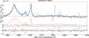 |
Fig. A.2. SDSSJ1427-0029. Same as in Fig. 2 but for an integrated spectrum with an aperture of 2 pixels. |
All Tables
All Figures
|
Fig. 1. Distribution of the Lyα nebulae around the targets in our sample in the velocity dispersion–size plane. The gray dots represent the parent sample from which our sources were selected, namely Arrigoni Battaia et al. (2019) (FAB+19) and Cai et al. (2019). Triangular and diamond markers indicate the targets selected for our study at z ∼ 2 and z ∼ 3, respectively. The points are color coded by bolometric luminosity, Lbol. |
| In the text | |
|
Fig. 2. Modeling of the integrated spectrum with an aperture of one pixel around the quasar center. Top: Total spectral profile (solid blue line) and its individual components. The orange line represents the [O III] λ4959, 5007 NLR component. The green line represents the outflowing component in the [O III] λ4959, 5007 line. The Hβ line is modeled with a broad component for the BLR shown in purple, a narrow component for the NLR shown in brown, and an additional broad component for the outflowing gas in pink. The FeII emission is shown in gray, and the linear continuum is shown in red. Bottom: Residuals of the total fit. The gray-shaded bands in both panels correspond to remnant sky emission after applying the sigma-clipping algorithm mentioned in Sect. 4.1.1. |
| In the text | |
|
Fig. 3. Optimally extracted SB maps of the Lyα nebulae surrounding the quasars (see Sect. 4.2). The white, gray, and black contours represent 2σ, 5σ, and 10σ, respectively. The values of σ are reported in Table 2. The green cross in the center represents the position of the quasar, determined by estimating the photocentroid of a channel map in a wavelength where the Lyα line is not present. North is up; east is left. |
| In the text | |
|
Fig. 4. Lyman-α SB radial profiles. The red points show the average SB per radial annulus, while the gray line denotes the 2σ detection limit estimated for each annulus. |
| In the text | |
|
Fig. 5. Curve of growth of the [O III] (blue) and BLR normalized flux (red) in log scale. Targets Q0050+0051, Q0052+0140, and SDSSJ2319-1040 show evidence of spatially resolved [O III] emission. |
| In the text | |
|
Fig. 6. Median maps of the residual [O III] emission after PSF subtraction. Targets Q0050+0051, Q0052+0140, Q2123-0050, and SDSSJ2319-1040 show evidence of extended [O III] emission. The magenta, red, and cyan contours represent 5σ, 10σ, and 30σ contours of the Lyα SB maps, respectively. The white cross represents the AGN center. North is up; east is left. |
| In the text | |
|
Fig. 7. Flux and kinematics maps of the [O III] emission for the targets showing spatially resolved and/or extended emission. The first column shows the flux map of the [O III] emission. The second, third, and fourth columns show the v10, v90, and w80 velocity maps, respectively. The black cross marks the AGN center. North is up; east is left. |
| In the text | |
|
Fig. 8. Relation between outflow kinetic power and Lyα nebulae size. |
| In the text | |
|
Fig. 9. Relation between outflow kinetic power and Lyα nebulae luminosity. |
| In the text | |
|
Fig. 10. Velocity map, v50, of Q0050+0051. |
| In the text | |
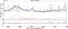 |
Fig. A.1. Q2121+0052. Same as in Fig. 2 but for an integrated spectrum with an aperture of 2 pixels. |
| In the text | |
|
Fig. A.2. SDSSJ1427-0029. Same as in Fig. 2 but for an integrated spectrum with an aperture of 2 pixels. |
| In the text | |
Current usage metrics show cumulative count of Article Views (full-text article views including HTML views, PDF and ePub downloads, according to the available data) and Abstracts Views on Vision4Press platform.
Data correspond to usage on the plateform after 2015. The current usage metrics is available 48-96 hours after online publication and is updated daily on week days.
Initial download of the metrics may take a while.