| Issue |
A&A
Volume 707, March 2026
|
|
|---|---|---|
| Article Number | A255 | |
| Number of page(s) | 13 | |
| Section | Interstellar and circumstellar matter | |
| DOI | https://doi.org/10.1051/0004-6361/202557944 | |
| Published online | 17 March 2026 | |
ALMA Band 1 observations of the ρ Oph W filament
I. Enhanced power from excess microwave emission at high spatial frequencies
1
Departamento de Astronomía, Universidad de Chile,
Casilla 36-D,
Santiago,
Chile
2
Data Observatory Foundation,
Eliodoro Yáñez 2990,
Providencia,
Santiago,
Chile
3
Núcleo de Astroquímica, Facultad de Ingeniería, Universidad Autónoma de Chile,
Av. Pedro de Valdivia 425,
Providencia,
Santiago,
Chile
4
University of Santiago of Chile (USACH), Faculty of Engineering, Computer Engineering Department,
Chile
5
Institut d’Astrophysique Spatiale (IAS), Université Paris-Saclay, CNRS,
Bâtiment 121,
91405
Orsay Cedex,
France
6
Institut de Recherche en Astrophysique et Planétologie (IRAP),
Toulouse,
France
★ Corresponding author: This email address is being protected from spambots. You need JavaScript enabled to view it.
Received:
2
November
2025
Accepted:
2
February
2026
Abstract
Context. The ρ Oph W photo-dissociation region (PDR) is an example source of bright excess microwave emission (EME), over synchrotron, free-free, and the Rayleigh-Jeans tail of the sub-millimetre (sub-mm) dust continuum. Its filamentary morphology follows roughly that of the IR poly-cyclic aromatic hydrocarbon (PAHs) bands. The EME signal in ρ Oph W drops abruptly above ~30GHz and its spectrum can be interpreted in terms of electric-dipole radiation from spinning dust grains (or ‘spinning dust’).
Aims. Deep and high-fidelity imaging and spectroscopy of ρ Oph W may reveal the detailed morphology of the EME signal, free from imaging priors, while also enabling a search for fine structure in its spectrum. The same observations may constrain the spectral index of the high-frequency drop.
Methods. An ALMA Band 1 mosaic yields a deep deconvolved image of the filament at 36-44 GHz, which we used as template for the extraction of a spectrum via cross-correlation in the uv plane. Simulations and cross-correlations on near-infrared ancillary data yield estimates of flux loss and biases.
Results. The spectrum is a power law, with no detectable fine structure. It follows a spectral index α = −0.78 ± 0.05, in frequency, with some variations along the filament. Interestingly, the Band 1 power at high spatial frequencies increases relative to that of the IR signal, with a factor of two more power in Band 1 at ~20" than at ~100 " (relative to IRAC 3.6 μm). An extreme example of such radio-only structures is a compact EME source, without an IR counterpart. It is embedded in strong and filamentary Band 1 signal, while the IRAC maps are smooth in the same region. We provide multi-frequency intensity estimates for spectral modelling.
Key words: radiation mechanisms: general / protoplanetary disks / stars: individual: rho Oph W / photon-dominated region (PDR) / radio continuum: ISM / ISM: individual objects
© The Authors 2026
 Open Access article, published by EDP Sciences, under the terms of the Creative Commons Attribution License (https://creativecommons.org/licenses/by/4.0), which permits unrestricted use, distribution, and reproduction in any medium, provided the original work is properly cited.
This article is published in open access under the Subscribe to Open model. This email address is being protected from spambots. You need JavaScript enabled to view it. to support open access publication.
1 Introduction
Cosmic microwave background (CMB) anisotropy experiments identified an anomalous diffuse Galactic foreground in the range 10-90 GHz (Kogut et al. 1996; Leitch et al. 1997), which was confirmed, in particular, by the WMAP (Gold et al. 2011) and Planck missions (Planck Collaboration XX 2011; Planck Collaboration I 2016a). As reviewed in Dickinson et al. (2018), this diffuse emission is correlated with the infrared (IR) thermal emission from dust grains on large angular scales and at high Galactic latitudes. The spectral index in specific intensity (Iν ∝ να) of the anomalous Galactic foreground is α ~ 0 in the range 15-30 GHz (Kogut et al. 1996), but any semblance to optically thin free-free is dissipated by a drop between 20-40 GHz, with α~ −0.85 for high-latitude cirrus (Davies et al. 2006).
Bright centimetre (cm) wavelength radiation has been reported from a dozen well-studied molecular clouds, with intensities that are well in excess of the expected levels for free-free, synchrotron, or the Rayleigh-Jeans tail of the sub-mm dust emission (e.g. Finkbeiner et al. 2002; Watson et al. 2005; Casassus et al. 2006; Scaife et al. 2009, 2010; Castellanos et al. 2011; Vidal et al. 2011; Tibbs et al. 2012; Vidal et al. 2020; Cepeda-Arroita et al. 2021). A common feature of all cm-bright clouds is that they host conspicuous photo-dissociation regions (PDRs). The Planck mission picked up spectral variations in this excess microwave emission (EME) from source to source along the Gould Belt, where the peak frequency is νpeak ~ 26 - 30 GHz, while νpeak ~ 25 GHz in the diffuse ISM (Planck Collaboration XII 2013; Planck Collaboration X 2016b).
The prevailing interpretation for EME, also called anomalous microwave emission (AME), is electric-dipole radiation from spinning very small grains, or ‘spinning dust’ (Draine & Lazarian 1998). A comprehensive review of all-sky surveys and targeted observations supports this spinning dust interpretation (Dickinson et al. 2018). The carriers of spinning dust remain to be identified, however, and could be poly-cyclic aromatic hydrocarbons (PAHs) (Ali-Haïmoud 2014), nano-silicates (Hoang et al. 2016; Hensley & Draine 2017), or spinning magnetic dipoles (Hoang & Lazarian 2016; Hensley & Draine 2017). Nano-silicates have, however, been excluded as the sole source of the EME in the diffuse ISM (i.e. in Planck all-sky maps, Ysard et al. 2022). A contribution to EME from the (vibrational) thermal emission of magnetic dust (Draine & Lazarian 1999) may be important in some regions (Draine & Hensley 2012).
Independent modelling efforts of spinning dust emission reach similar predictions, for given dust parameters and local physical conditions (Ali-Haïmoud et al. 2009; Hoang et al. 2010; Ysard & Verstraete 2010; Silsbee et al. 2011; Zhang & Chluba 2025). In addition, thermochemical PDR models estimate the local physical conditions that result from the transport of ultraviolet (UV) radiation (Le Petit et al. 2006). Therefore, observations of the cm-wavelength continuum in PDRs, and especially its variations, can potentially calibrate the spinning dust models and help identify the dust carriers. Eventually, the radio continua from PDRs may provide constraints on physical conditions under the spinning-dust hypothesis.
Cosmic Background Imager (CBI) observations have shown that the surprisingly bright cm-wavelength continuum from the nearby ρ Oph molecular complex peaks in the ρ Oph W PDR (Casassus et al. 2008; Arce-Tord et al. 2020). The WMAP and Planck spectral energy distributions (SEDs) are fit by spinning dust models (Casassus et al. 2008; Planck Collaboration XX 2011), which also account for the low frequency tail (at 10 GHz, González-González et al. 2025). However, the CBI maps revealed that the radio-IR correlation breaks down when resolving the molecular complex. Under the spinning dust hypothesis, this points at environmental factors that strongly increase the spinning dust emissivity per nucleon (j1cm/nH) in ρ Oph W, by a factor of at least 26 relative to the mid-IR (MIR) peak in the whole complex (Arce-Tord et al. 2020).
Australia Telescope Compact Array (ATCA) observations of ρ Oph W resolved the width of the filament (Casassus et al. 2021b). The multi-frequency 17-39 GHz mosaics showed morphological variations in the cm-wavelength continuum. The corresponding spectral variations can be interpreted in terms of the spinning dust emission mechanism as a minimum grain size cutoff at 6 ± 1 Å, that increases deeper into the PDR. This interpretation is strengthened by the qualitative agreement with a PAH size proxy. It is also consistent with the conclusions of studies of the Orion Bar, based on near- to far-IR (NIR-FIR) JWST data, which take into account radiative transfer through PDRs (Elyajouri et al. 2024).
The ATCA observations of ρ Oph W point at EME spectral variations within a single source. Such spectral variations may be key to calibrate spinning dust models and to identify the carriers and their spin-up mechanism. However, with only five antennas, the ATCA 39 GHz data are noisy and strongly affected by flux loss due to missing spatial frequencies (i.e. source angular size much larger than the maximum recoverable scale). In addition the PDR peak at 39 GHz is contaminated by the SR 4 point source, which is difficult to remove at the angular resolution of the ATCA data (the width of the filament is only a couple of beams).
The commissioning of the Band 1 receivers on the Atacama Large Millimetre Array (ALMA), covering 35-50 GHz, offers the opportunity to map the filament with much better fidelity than with ATCA, and at finer angular resolutions. ALMA can also map the cm-wavelength spectral index across the PDR, which, combined with the ATCA 17 and 20 GHz data, could allow for an exploration into the spinning dust parameter space.
The same ALMA observations can be used to search for fine structure in the EME spectrum, and identify its carriers (potentially through the detection of PAH combs, Ali-Haïmoud 2014; Ali-Haïmoud et al. 2015). The Band 1 data also allow to place limits on carbon recombination lines (CRRLs). One of the spin-up mechanism is plasma drag (i.e. encounters with H+ and C+ ions), which requires the EME to be coincident with the C II region in the PDR.
Here, we report on mosaic observations of ρ Oph W in ALMA Band 1 at ~7 arcsec resolution (or twice as fine as the 39 GHz ATCA data). Section 2 summarises our observations as well as our strategies for imaging and point-source subtraction. Section 3 presents the extraction of the Band 1 spectra, a compilation of the multi-frequency SEDs, and a discussion of the limits on any fine structure in the spectrum, both on PAH combs and CRRLs. Section 4 gives our conclusions. An interpretation of the measured SEDs in terms of the spinning dust hypothesis will be presented in a companion article.
2 Observations
2.1 The ρ Oph W filament and the breakdown of the radio-IR correlation
The region of the ρ Ophiuchi molecular cloud exposed to UV radiation from HD 147889 (i.e. ρ Oph W) is among the closest examples of PDRs, located at a distance of 138.9 pc. It is seen edge-on and extends over ~10×3 arcmin. It has been extensively studied in the FIR atomic lines observed by ISO (Liseau et al. 1999; Habart et al. 2003).
The ρ Oph complex is a region of intermediate-mass star formation (White et al. 2015; Pattle et al. 2015). It does not host a conspicuous HII region, in contrast to the Orion Bar, another well-studied PDR, where the UV fields are ~100 times stronger. While the HD 147889 binary has the earliest spectral types in the complex (B2IV and B3IV, Casassus et al. 2008), the region also hosts two other early-type stars: S 1 (also a binary including a B4V primary, Lada & Wilking 1984) and SR 3 (with spectral type B6V, Elias 1978). Both S 1 and SR 3 are embedded in the molecular cloud. Figure 2 of Arce-Tord et al. (2020) provides an overview of the region, including the relative positions of these three early-type stars.
Interestingly, the peak at all IR wavelengths, i.e. the circumstellar nebula around S 1, is undetectable in the CBI data. Upper limits on the S 1 flux density and correlation tests with Spitzer -IRAC 8 μm rule out a linear radio/IR relationship within the CBI 45 arcmin primary beam (which encompasses the bulk of the molecular cloud mass). This breakdown of the radio-IR correlation in the ρ Ophiuchi complex is further pronounced at finer angular resolutions, with observations from the CBI 2 upgrade to CBI (Arce-Tord et al. 2020).
Thus, while the cm-wavelength and NIR-MIR signals in the ρ Oph W filament display a tight correlation (as expected for EME), this correlation breaks down in the ρ Oph complex as a whole, when including the circumstellar nebula around S 1. The brightest IR PAH emission bands are observed near S 1, but this region is undetectable at 31 GHz.
The breakdown of the radio-IR correlation suggests that cross-correlation techniques are of limited use in the interpretation of the EME signal in ρ Oph. Such cross-correlations have successfully been applied to all-sky surveys, since the diffuse EME signal can be described in terms of average physical conditions and dust properties. However, in a PDR interface, the conditions are not homogeneous.
2.2 Data acquisition
The ALMA Band 1 observations of ρOphW were acquired in ALMA program 2023.1.00265.S using the 12m array. An observation log is provided in Table 1. The correlator was tuned to four spectral windows (spws), centred on 37.209 GHz, 39.146GHz, 41.167GHz, and 43.104GHz, with 1920 channels each. The channel width was set to 976.562 kHz, providing a bandwidth of 1.875 GHz per spw. The data from the last execution block, on 14-Mar-2024, were corrupted in several ways and were not included in the analysis.
The data were calibrated by staff from the North America ALMA Regional Center, using CASA version 6.5.4.9 and ALMA pipeline version 2023.1.0.124. Full details on the calibration can be obtained through the ALMA science archive, in the quality assurance reports. In brief, some flagging was applied, in particular to a channel at 43.91 GHz and to antenna DV05 for spw 39.146 GHz. The phase and pointing calibrator was J1625-2527, while the band pass and flux calibrator was J1617-5848.
Observation log.
 |
Fig. 1 ALMA Band 1 continuum imaging of the ρ Oph W filament. Each image is shown in linear stretch, and x- and y- axis are offset along RA and Dec from J2000 16:25:57.0 −24:20:48.0. (a) Restored image, in natural weighting, after point-source subtraction, with a beam of 8".696×6".436/-86deg (see text), and a noise of 5.55 μJy beam−1. (b) Same as panel a, but before point-source subtraction. The three bright point sources are the young stellar objects SR 4 near the centre, ISO-Oph-17 to the east, and DoAr 21 to the south. The cyan circles are centred on the phase directions of each field and their radii correspond to half the radius of the first Airy null (corresponding to a primary beam attenuation of ~0.34). (c) Deconvolved model image, Im, after point-source subtraction and with 1"2 pixels. |
2.3 Imaging
The central region of the ρ Oph W filament was covered in a mosaic of K = 16 fields, as shown in Fig. 1b. Imaging was performed as an instance of the maximum-entropy method, by fitting a model image, covering N = 10242 pixels, 1″2 each, directly to the visibility data. We used the gpu-uvmem package (Casassus et al. 2006; Cárcamo et al. 2018) to minimise the objective function,
 (1)
(1)
where  is the weight associated to each visibility datum Vk,l, and Lk is the total number of visibilities for field k. The model visibilities
  are computed on the model image Im (xi). The free parameters are the intensities in each image pixel in units of a fiducial noise value,
  , where σI = 100 μJy beam−1 was chosen to be large as a preconditioning factor for the optimisation. The theoretical noise of the natural-weights dirty map is 1.53 μJy beam−1, with a beam of 8″.70×6″.44/-85.6 (in the format major axis × minor axis / position angle).
The model visibilities, Vm, are computed from the model image Im using the Airy-disk approximation to the ALMA primary beam (Remijan et al. 2019), and by propagating the model image to each frequency using a flat spectral index in flux density (α = 0). No visibility gridding was used. Image restoration was carried out by producing a linear mosaic of the residual dirty maps, in natural weights, and by adding the model image smoothed by the Gaussian beam. The linear mosaic introduces an attenuation map A(x) (e.g. Eqs. (A8) and (A9) in Casassus et al. 2021b).
The regularisation parameter λ in Eq. (1) allows for smoother model images than pure χ2 reconstructions, which tend to fit the noise. Trials resulted in satisfactory results for λ = 0.1, with thermal residuals. The corresponding images are shown in Fig. 8. However, with entropy regularisation, the spectral extraction technique turned out to be significantly biased (see Appendix A).
We therefore opted to set λ = 0 and truncated the optimisation at ten iterations to avoid excessive clumping.
The resulting model image, Im, that fits the visibility data in a pure least-squares sense, is shown in Fig. 1 (but after pointsource subtraction; see Sect. 2.4 below). We note that this image has not been convolved or smoothed in any way. Its effective angular resolution is about one-third the natural-weight clean beam (e.g. Casassus et al. 2021a, and references therein).
Systematics in synthesis imaging are particularly strong when the longest dimension of the source are resolved-out. In the case of the ATCA observations, with five antennas and, hence, a very sparse uv-coverage, we relied on the IRAC 8 μm image as a prior to recover the missing interferometer spacings. This choice was justified by the very tight 8 μm-radio correlation at 17 and 20 GHz. However, at higher frequencies the radio filament is shifted parallel to its signal at IRAC 8 μm. Still, with ~39 antennas and high-fidelity imaging, ALMA recovers the ρ Oph W filament without the need of a prior, but with significant flux loss. As described in Appendix A, the flux recovered over the whole mosaic is ~30%.
Point source flux densities and spectral indices at 40.15 GHz.
2.4 Point-source subtraction
There are three bright point sources in the mosaic of ρ Oph W, corresponding to the young stellar objects SR4, ISO-Oph-17, and DoAr21. These were subtracted in the uv plane, handling the raw (non-gridded) visibility data with the pyralysis package (Casassus & Cárcamo 2022). We first fit for the point source positions, their flux densities, Fνo, at the reference frequency, νo = 40.15 GHz (corresponding to the centre frequency of the four spectral windows), and spectral indices, α. In order to reduce the volume of the data, we averaged the visibilities into 60 channel bins (using CASA task mstransform). The pointsource fits were carried out for each execution block separately, and selecting the fields closest to each point source. We used the iminuit package (James & Roos 1975; Dembinski et al. 2020), using the Hessian approximation to estimate uncertainties. Provided with models for each point source, we proceeded with their subtraction from the non-channel-averaged visibilities.
The imaging of the point-source-subtracted dataset shown in Fig. 1a offers satisfactory results. The point-source fits to DoAr 21 required the incorporation of the four nearest fields to reach thermal residuals. We attribute the imperfect point-source subtraction for DoAr 21 in single-field point-source fits (with ≲5% residuals) to the accuracy of the Airy disk approximation to the ALMA primary beam.
As summarised in Table 2, the flux densities for ISO-Oph 17 and SR 4 were consistent in each execution block, with no indication of variability. The spectral indices for these two sources are consistent with the Rayleigh-Jeans tail of the sub-mm dust continuum. However, the very bright non-thermal emission from DoAr 21 turned out to be highly variable. This star is known to be a compact binary. VLBA astrometric monitoring is consistent with two sub-stellar companions in external orbits (Curiel et al. 2019). DoAr 21 has no detectable disk in the sub-mm continuum (Cieza et al. 2019). Our measurements for DoAr 21 are summarised in Fig. 2.
As a sanity check on the point-source fits (and provided with their best-fit positions, x0), we also extracted point-source flux densities in each channel. We selected the closest field to each source, and obtained the point-source flux densities with
![Mathematical equation: F_\nu = \frac{\sum_{l=1}^{L_k} \omega_{k,l}~ \Re\left[ V_{k,l} e^{-2\pi i \vec{u}_{k,l}\cdot\vec{x_\circ}}\right] }{ \mathcal{A}_k(\vec{x_\circ}) \sum_{l=1}^{L_k} \omega_{k,l} } ,](/articles/aa/full_html/2026/03/aa57944-25/aa57944-25-eq5.png) (2)
(2)
where K represents the real part, Ak is the primary-beam attenuation pattern for field k, and uk,l is the uv plane coordinate for datum Vk,l. The associated errors are
 (3)
(3)
Example spectra, extracted over all epochs, are shown in Figs. 3 and 4, for DoAr 21 and SR4. The spectral index fits from Table 2 are consistent with the channel flux densities.
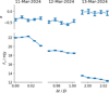 |
Fig. 2 Point source fits to DoAr 21, over individual interferometer scans, each ~ 10 min long. The top and bottom rows respectively record spectral index, α, and flux density, Fν, at the reference frequency of 40.15 GHz. The x-axis gives the Julian date, expressed in days from the start of the observations. |
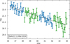 |
Fig. 3 Flux densities for DoAr 21, on 11-Mar-2024, extracted over 120-channel averages. The black line is the best fit point-source model from Table 2. Spectral windows are plotted in alternating colours. |
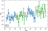 |
Fig. 4 Flux densities for SR4, extracted over 120-channel averages. The black line is the best fit point-source model from Table 2. Spectral windows are plotted in alternating colours. |
2.5 Self-calibration trials
As explained in Appendix B, after point-source subtraction gpu-uvmem generates images with much higher dynamic range than achievable with CASA-tclean. However, gpu-uvmem does not perform as well for extended signal in the vicinity of bright point sources. We therefore attempted self-calibration of the 60-channel average data, using the gpu-uvmem model visibilities for the extended signal, but with the addition of the point-source best fits. Given the variability of DoAr 21, this trial was attempted in individual execution blocks. We performed a single iteration of tasks gaincal and applycal, using phase-only gain calibration, and without additional flagging. Imaging with gpu-uvmem for the 11-Mar-2024 execution block, after point-source subtraction, yielded a peak signal of 733 μJy beam−1 and a noise level of 7.2 μJy beam−1 (or a signal-to-noise ratio of S/N=101.81 (for a beam of 8″.912 × 6″.050). For comparison, before self-calibration the same restoration yields essentially the same value, with a somewhat larger S/N=101.96. We concluded that self-calibration was not necessary for this dataset.
3 Analysis and discussion
3.1 Limits on carbon recombination lines
There are four carbon radio-recombination lines (CRRLs) within our correlator setup, from C56α to C53α. The turbulent linewidths in the filament are likely of the order of ~2km s−1 (Pankonin & Walmsley 1978); thus, they are narrower than the channel width of ~7km s−1. We stacked all four lines in a joint imaging and obtained a limit of 0.15 mJy beam−1, with a 8″.81 × 6″.53 beam. The physical conditions in ρ Oph W inferred from PDR models (Habart et al. 2003) should yield LTE line intensities of ~2mJy beam−1 (at ~300K, Casassus et al. 2021b). Depopulation factors are negligible above 100 K (Salgado et al. 2017). The non-detection of CRRLs is surprising and might be due to collisional de-excitation of the denser regions in the filament, resulting in an unstructured map, which might have beeen filtered out in the interferometer observations.
3.2 Extraction of the intra-band diffuse emission spectrum
The diffuse emission from ρ Oph W is too faint for the extraction of its spectrum in individual channels through aperture photometry. Instead, we opt for cross-correlation with a template image, for which we use the deconvolved model image, Im, of Fig. 1c, assuming a flat spectral index. We search for a linear-regression slope, aν, such that
 (4)
(4)
by simulating visibilities on the template image,  (using the pyralysis package, Casassus & Cárcamo 2022), and minimising
 (5)
(5)
where the sum is restricted to the Mk < Lk visibilities at frequency ν and for field k. The result is
![Mathematical equation: a_\nu & = & \frac{ \sum_{k=1}^{K} \sum_{l=1}^{M_k} \omega_{k,l} \Re{\left[ V_{k,l}^{\ast} V^m_{k,l} \right] } }{\sum_{k=1}^{K} \sum_{l=1}^{M_k} \omega_{k,l} \left| V^m_{k,l} \right|^2 }, \\](/articles/aa/full_html/2026/03/aa57944-25/aa57944-25-eq10.png) (6)
(6)
 (7)
(7)
The cross-correlation technique used here mitigates against the effect of flux loss or missing spatial frequencies in images reconstructed from interferometric data. A residual bias is still expected in the determination of spectral slopes, since uv-coverage varies with frequency. This bias is studied in Appendix A. In pure-χ2 imaging (i.e. without the introduction of entropy regularisation as per Eq. (1)), this residual bias in spectral slope is negligible. It does, however, become detectable with the introduction of entropy, which is the reason we avoided regularisation.
Example spectra are shown in Fig. 5 for the 120-channel average and extracted over regions along the filament. Power-law fits for
 (8)
(8)
yield varying spectral indices, αd, over different regions. The spectral index variations are very significant along the filament, from αd = −0.16 ± 0.14 in fields 5 and 6 (south-east of the filament), to αd = −1.06 ± 0.08 in fields 7-10 (north-west of the filament). The slopes aνo are slightly biased downwards, with aνo = 0.96 ± 0.005 for νo = 36.63 GHz averaged over all fields, which results from the use of the pure-χ2 model image as template. In pure χ2 imaging, the model image fits the noise to some extent, which leads to positive-definite noise that then acts as extra signal in the simulated channel visibilities. The same exercise using entropy regularisation, with λ = 0.1, results in aν value that is consistent with 1, but at the expense of a bias in αd (see Appendix A).
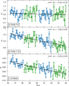 |
Fig. 5 Spectrum of the diffuse emission from ρ Oph W, as estimated with the cross-correlation slope, aν. The black line is the best-fit powerlaw spectrum, with spectral index indicated in the legends. Plots a-c correspond to spectra extracted over different parts of the mosaic, as indicated in each plot. Field IDs follow from Fig. 1. Spectral windows are plotted in alternating colours. |
3.3 Cross-correlations with the Spitzer-IRAC maps
As previously noted, the cm-wavelength continuum in ρ Oph W is closely correlated with the NIR emission, in particular as traced in the four bands of the Infrared Array Camera (IRAC) aboard Spitzer (as provided by the c2d Spitzer Legacy Survey Evans et al. 2009). The IRAC images were obtained from the Set of Enhanced Imaging Products (SEIP)1, which is part of the Spitzer Heritage Archive. Point sources were removed prior to using the IRAC maps as cross-correlation templates for radio interferometric simulations. Details on IR point-source subtraction are given in Appendix C.
We quantified the degree of correlation between the ALMA Band 1 data and the IRAC bands using linear regression and the Pearson r cross-correlation coefficient. IRAC angular resolutions are 1″.66, 1″.72, 1″.78, and 1″.98 at 3.6, 4.5, 5.6, and 8.0 μm, respectively (Fazio et al. 2004). Since most of the 40.2 GHz signal is in the shortest spacings, and the angular resolution of the ALMA map is ~7 arcsec, biases in the correlations due to the coarser resolution at 8.0 μm are negligible.
As in Sect. 3.2, the radio-IR slope, aIR, in specific intensities, IBand 1 = aIRIIRAC, is given by
![Mathematical equation: a_{\rm IR} = \frac{\sum_{k=1}^{K} \sum_{l=1}^{L_k} \omega_{k,l} \Re\left[V^*_{k,l} V^{\rm IRAC}_{k,l}\right]}{\sum_{k=1}^{K} \sum_{l=1}^{L_k} \omega_{k,l} \left|V^{\rm IRAC}_{k,l}\right|^2},](/articles/aa/full_html/2026/03/aa57944-25/aa57944-25-eq13.png) (9)
(9)
where  are the visibilities extracted on a simulation of the Band 1 uv-coverage on the (point-source-subtracted) IRAC maps, obtained with the pyralysis package. The associated 1σ uncertainty is given by error propagation,
 (10)
(10)
The radio-IR cross-correlation is
 (11)
(11)
where the mean observed visibility is
 (12)
(12)
and likewise for the simulated visibilities  . The standard deviation of the Band 1 data is
 (13)
(13)
and likewise for σVIRAC. Finally, an expression for the Pearson coefficient adapted to the case of complex visibility data is
 (14)
(14)
The uncertainty on r vanishes when computed over large samples, which limits its use in discriminating between templates. However, when taking the r values in uv-radius bins the uncertainties can become important for the larger uv-radii, because of the relative scarcity of long baselines in this Band 1 dataset. We estimated the uncertainties in r by bootstrapping.
Table 3 lists the radio-IR slopes averaged over all spectral windows and fields, and calculated after binning the data into 16 channels (with a 120 channel average). The r coefficients turned out to be dominated by noise and essentially zero when using all baselines. However, a cross-correlation signal is clear for short baselines, containing the bulk of the signal, as illustrated in Fig. 6.
The trends in aIR with uv-radius are summarised in Fig. 7a. Notably, the radio-IR slope increases with baseline length. For the best template (i.e. 3.6 μm), aIR increases from 3.3 × 10⁻² ± 1.8 × 10⁻⁴ to 5.83 × 10⁻² ± 2.8 × 10⁻³ for the bin starting at 7818λ. This corresponds to a factor of 1.77 ± 0.01. Relative to the IRAC power-spectrum, there is thus almost a factor of two more power in Band 1 at ~20″ than at ~100″. This confirms that the Band 1 and IRAC morphologies are appreciably different, and limits the use of the IRAC bands as templates to estimate the spectral index of the Band 1 signal, since varying frequencies correspond to varying uv-radii.
As shown in Fig. 7b, the r coefficients decrease strongly with baseline, which we attribute to the radio-IR correlation breakdown when resolving the EME sources, even within the ρ Oph W filament (see also Sect. 3.4 below). In addition, visibility measurements at longer baselines are less frequent, and hence such uv-radii bins are noisier. In this case, the r values between each IRAC band are indistinguishable beyond ~ 10 000λ. The template with highest r values is IRAC 3.6 μm, and the ratio in r between IRAC bands is greatest for uv-radii between 5000 and 7000 λ, corresponding to spatial scales of ~40″ to ~30″.
Radio-IR slopes for each IRAC band.
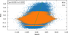 |
Fig. 6 Radio-IR linear regression in real and imaginary parts, with Band 1 visibilities on the x-axis, and simulated IRAC 3.6 μm visibilities on the y-axis. Axis units are given in Jy. Only data corresponding to uv-radii shorter than 2606λ have been selected. The green line corresponds to the best fit linear regression. |
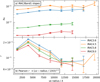 |
Fig. 7 Radio-IR slopes (in a) and Pearson r coefficient (in b) as a function of baseline length. The domain in uv-radius has been truncated at the maximum value for which the uncertainties become larger than a third of the reported values. |
3.4 A compact EME source with no IR counterpart
As mentioned in Sect. 3.3, the Band 1 power at high spatial frequencies increases relative to that of the IR signal. An example in the image plane may be the strong peak found at J2000 right ascension (RA) of 16:25:54.154 and delination (Dec) of −24:19:52.5, or about ~45″ north-west from the centre of images in Fig. 1a (at an offset of ∆α = −38″ along the RA and ∆δ = 55″ along the Dec). As shown in Fig. 8a, this local peak appears to be point-like in the Band 1 model image, and reaches 0.576 ± 0.005 mJy beam−1 in the restored image Fig. 8f, which rivals the global peak along the filament, at 0.631 ± 0.005 mJy beam−1 .
The compact EME source is smaller than the ~7″ beam, and bears no counterpart in the IRAC bands. It is embedded along strong and filamentary Band 1 signal, which bends by ~60 deg from the PDR plane. Interestingly, this thin filament is absent from the IR maps, which instead appear smooth and fainter relative to the peak. The Band 1 point source is not an artefact of the imaging strategy, as verified through simulations of the Band 1 uv-coverage on the IRAC images (Figs. 8g-j; see also Appendix A). The point source has no FIR counterpart either (Figs. 8k-o), as shown by comparison with images from the Herschel Gould Belt Survey (Ladjelate et al. 2020).
3.5 Comparison with the ATCA mosaics
In the ATCA observations (Casassus et al. 2021b), at 30 arcsec resolutions, the 17-20 GHz intensities tightly follow the MIR, i.e. Icm ∝ I(8 μm), despite the breakdown of this correlation on larger scales. However, while the 33-39 GHz filament is parallel to IRAC 8 μm, it is offset by 15-20 arcsec towards the UV source. This effect is also picked-up in the Band 1 40.2 GHz observations, as shown in Fig. 9.
The blue-ward shift of the EME spectrum on the edge of the PDR closer to HD 147889 can be related to a gradient in physical conditions or grain properties. In particular, the trends in the ATCA data were reproduced in the spinning dust hypothesis, in terms of a gradient in minimum grain size, increasing deeper in the cloud (Casassus et al. 2021b).
The present ALMA data cannot, however, be used to constrain resolved gradients in physical conditions across the PDR. As explained below, the Band 1 observations must be corrected for flux loss to build a multi-frequency SED, which can only be achieved, to a reasonable accuracy, on scales corresponding to the primary beam. The Band 1 spectral index measurements are also extracted over such large scales. The combination of 7 m (ALMA Compact Array) observations with the present 12 m observations could allow for such a resolved multi-frequency analysis.
3.6 Spectral energy distribution
Given the interferometer filtering, it is difficult to extract SEDs on small scales; namely, of a single synthesised clean beam or ~7″. Instead, we opt to build SEDs on scales of a primary beam, which also allows estimates of the Band 1 spectral index. The total Band 1 flux densities are estimated via aperture photometry, and by correcting for the flux loss due to missing interferometer spacings, for which we use the simulations on the IRAC 3.6 μm template (see Appendix A). This correction depends on the chosen photometric aperture. The thermal errors are negligible compared to absolute flux calibration errors, and we opt to consider a fixed 10% error on the flux densities extracted for the radio data.
The IR and FIR SEDs were built from the IRAC and Herschel images. The flux densities from the IR ancillary data were extracted by aperture photometry; namely, by integrating the product of the IR images with the linear mosaic attenuation map (see Appendix A).
The ATCA images reported in Casassus et al. (2021b) already fill in the missing spatial frequencies by incorporation of prior images in the synthesis imaging strategy. We therefore proceeded similarly as for the IR ancillary data, with the choice of smaller apertures to accommodate the ATCA mosaics (see Fig. 9). The resulting SEDs are tabulated in Table 4. Plots for these SEDs and model comparisons will be presented in a companion article.
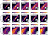 |
Fig. 8 Comparison of the ALMA Band 1 with IR templates. Insets highlight the compact EME source at J2000 RA 16:25:54.154, Dec −24:19:52.5. The blue contour traces the Band 1 image from Fig. 1a at 80% peak. (a) Band 1 deconvolved image (same as Fig. 1c, but with λ = 0.1 for comparison). (b-e) IRAC images, with 1″ pixels, and before point-source subtraction. (f) Restored Band 1 image (same as Fig. 1a, but with λ = 0.1). (g-j) Restorations of the IRAC simulations, after point-source subtraction, scaling by aIR, and addition of thermal noise, as in the Band 1 data. (k-o) Herschel images. |
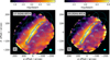 |
Fig. 9 Comparison of the 17.5 GHz (in a) and 20.2 GHz (in b) ATCA mosaics (from Casassus et al. 2021b) with the ALMA Band 1 pointings. The Band 1 restored image from Fig. 1a is overlaid in a single contour at 60% peak intensity. |
3.7 Limits on PAH combs
The new ALMA observations can also be used to search for fine structure in the spinning dust spectrum. If due to quasi-symmetric PAHs, the EME may be structured with evenly spaced combs of rotational lines, separated by ∆ν ~ 1 MHz (Ali-Haïmoud 2014; Ali-Haïmoud et al. 2015). The exact spacing, ∆ν, can be derived from the PAH rotational constant and inversely proportional to the grain moment of inertia, which is itself a measure of the number of carbon atoms in the PAHs. Such comb-like fine structures in the EME spectrum would confirm the spinning dust hypothesis and would identify the carriers (as performed in TMC-1 for small PAHs, McGuire et al. 2018, 2021).
As shown by Ali-Haïmoud (2014), the rotational spectrum of imperfect planar PAHs, with either D6h or D3h quasi-symmetry and a permanent dipole arising from defects2, should appear as a regularly spaced frequency comb,
 (15)
(15)
with
 (16)
(16)
to first order in defects and where I3 is the largest moment of inertia. This principal moment of inertia can be related to the number of carbon atoms, NC, in the PAH (Ali-Haïmoud 2014), via
 (17)
(17)
We use the cross-correlation spectrum, aν, to place limits on such PAH combs in an adaptation of the matched-filter technique proposed in Ali-Haïmoud (2014) and Ali-Haïmoud et al. (2015). A function f (ν' is decomposed into a basis of comb-like functions, ci, and its projection onto a particular comb is
 (18)
(18)
where the dot product of two functions is
 (19)
(19)
and  .
.
In this application, the domain of the comb basis is split into S = 4 spectral windows, each composed of C = 1920 regularly-spaced channels and with channel widths. δνs. The comb, cνs, for a spacing, ∆νline, in spectral window, s, is generated with the following algorithm,
 (20)
(20)
where ⌉ is the nearest integer,
 (21)
(21)
define  if
if
 (22)
(22)
and  otherwise. The comb is given by
 (23)
(23)
We first rectify the signal aν by division with the power-law fit of Eq. (8),
 (24)
(24)
and correct for zero mean,
 (25)
(25)
The dot product with the comb basis is
 (26)
(26)
In summary, the projection of the rectified signal, δb(νs,c, on comb cj with line spacing ∆νline, is
 (27)
(27)
with an uncertainty of
 (28)
(28)
The significance, S(δb)/σ(S(δb)), is a measure of the power on a comb basis, defined by the line interval ∆νline. We scan ∆νline over the interval from twice the frequency resolution of aν (i.e. the channel width, or its binned versions), and up to 200 MHz, sampling every tenth of a resolution element. Figure 10 illustrates the resulting values for the case of five-channel bins and no channel binning.
There is no significant power in comb functions, with a spectral resolution as fine as twice the channel width: S(δb)/σ(S(δb)) < 3.5 in ~2000 values for ∆νline. Since the signal has been rectified and normalised, the uncertainty σ(S(∆νline)) directly gives the limit of fraction of signal in combs with spacing ∆νline, as summarised in Fig. 11. For example, in native spectral resolution, less than ~3 × 0.06 of the observed flux density from ρ Oph W is due to combs with spacing of ~200 MHz.
The absence of detectable fine-structure in the observed Band 1 spectrum may reflect a large number of possible configurations for a given number of carbon atoms (Tielens 2008). In addition, the most stable sub-nanometric particles are, a priori, neither flat nor symmetrical (Parneix et al. 2017; Bonnin et al. 2019). Furthermore, if the dipole moment is boosted by atom substitution or gain (or loss) of H atoms, each possible site of implantation would modify the moment of inertia and, thus, the comb. All these effects lead to the conclusion that there are so many weak lines superimposed that spectral structure cannot be detected, at least within the present limits (Fig. 11).
Broad-band SEDs for selected regions, defined by the Band 1 fields they comprise.
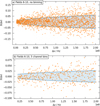 |
Fig. 10 Power S(δb) across a continuous range of combs with line intervals ∆ν. The top panel is for the raw spectral resolution, and the lower panel uses a five-channel average. Uncertainties are shown as vertical ±1σ error bars in blue (with total length of 2σ), and are offset to zero for clarity. |
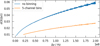 |
Fig. 11 Uncertainty on the projected power in a continuous range of combs with line intervals ∆ν. |
4 Conclusions
The ALMA observations of ρ Oph W, along with non-parametric imaging and visibility-plane correlations, allow estimates of the Band 1 flux density and spectral index of the EME in ρ Oph W. We place limits on the contribution from regularly spaced spectral combs and CRRLs. These spectral measurements will be analysed in terms of the spinning dust hypothesis in a companion article.
The Band 1 image of ρ Oph W reveals bends and clumps along the otherwise smooth IR filament. We compare the EME visibility power spectrum against that of IR templates. Interestingly, for the best template, i.e. IRAC 3.6 μm, there is almost a factor of two more power in Band 1 at ~20″ than at ~100″. An extreme of such radio-only structures is a compact source of pure EME, without any IR counterpart. It is embedded along strong and filamentary Band 1 signal, while the IRAC maps are featureless in the same region.
Acknowledgements
We thank the referee for constructive comments. S.C. and M.C. acknowledge support from Agencia Nacional de Investigación y Desarrollo de Chile (ANID) given by FONDECYT Regular grant 1251456, and ANID project Data Observatory Foundation DO210001. This paper makes use of the following ALMA data: ADS/JAO.ALMA2023.1.00265.S. ALMA is a partnership of ESO (representing its member states), NSF (USA) and NINS (Japan), together with NRC (Canada), NSTC and ASIAA (Taiwan), and KASI (Republic of Korea), in cooperation with the Republic of Chile. The Joint ALMA Observatory is operated by ESO, AUI/NRAO and NAOJ. This research has made use of data from the Herschel Gould Belt survey (HGBS) project (http://gouldbelt-herschel.cea.fr). The HGBS is a Herschel Key Programme jointly carried out by SPIRE Specialist Astronomy Group 3 (SAG 3), scientists of several institutes in the PACS Consortium (CEA Saclay, INAF-IFSI Rome and INAF-Arcetri, KU Leuven, MPIA Heidelberg), and scientists of the Herschel Science Center (HSC).
References
- Ali-Haïmoud, Y. 2014, MNRAS, 437, 2728 [Google Scholar]
- Ali-Haïmoud, Y., Hirata, C. M., & Dickinson, C. 2009, MNRAS, 395, 1055 [CrossRef] [Google Scholar]
- Ali-Haïmoud, Y., Pérez, L. M., Maddalena, R. J., & Roshi, D. A. 2015, MNRAS, 447, 315 [Google Scholar]
- Arce-Tord, C., Vidal, M., Casassus, S., et al. 2020, MNRAS, 495, 3482 [NASA ADS] [CrossRef] [Google Scholar]
- Bonnin, M. A., Falvo, C., Calvo, F., Pino, T., & Parneix, P. 2019, Phys. Rev. A, 99, 042504 [NASA ADS] [CrossRef] [Google Scholar]
- Cárcamo, M., Román, P. E., Casassus, S., Moral, V., & Rannou, F. R. 2018, Astron. Comput., 22, 16 [CrossRef] [Google Scholar]
- CASA Team, Bean, B., Bhatnagar, S., et al. 2022, PASP, 134, 114501 [NASA ADS] [CrossRef] [Google Scholar]
- Casassus, S., & Cárcamo, M. 2022, MNRAS, 513, 5790 [NASA ADS] [CrossRef] [Google Scholar]
- Casassus, S., Cabrera, G. F., Förster, F., et al. 2006, ApJ, 639, 951 [NASA ADS] [CrossRef] [Google Scholar]
- Casassus, S., Dickinson, C., Cleary, K., et al. 2008, MNRAS, 391, 1075 [NASA ADS] [CrossRef] [Google Scholar]
- Casassus, S., Christiaens, V., Cárcamo, M., et al. 2021a, MNRAS, 507, 3789 [CrossRef] [Google Scholar]
- Casassus, S., Vidal, M., Arce-Tord, C., et al. 2021b, MNRAS, 502, 589 [NASA ADS] [CrossRef] [Google Scholar]
- Castellanos, P., Casassus, S., Dickinson, C., et al. 2011, MNRAS, 411, 1137 [Google Scholar]
- Cepeda-Arroita, R., Harper, S. E., Dickinson, C., et al. 2021, MNRAS, 503, 2927 [NASA ADS] [CrossRef] [Google Scholar]
- Cieza, L. A., Ruíz-Rodríguez, D., Hales, A., et al. 2019, MNRAS, 482, 698 [Google Scholar]
- Curiel, S., Ortiz-León, G. N., Mioduszewski, A. J., & Torres, R. M. 2019, ApJ, 884, 13 [Google Scholar]
- Davies, R. D., Dickinson, C., Banday, A. J., et al. 2006, MNRAS, 370, 1125 [NASA ADS] [CrossRef] [Google Scholar]
- Dembinski, H., Pitiot, A., Schulz, C., et al. (2020). iminuit - A Python interface to MINUIT2. Zenodo. https://doi.org/10.5281/zenodo.3949207 [Google Scholar]
- Dickinson, C., Ali-Haïmoud, Y., Barr, A., et al. 2018, NewAR, 80, 1 [Google Scholar]
- Draine, B. T., & Hensley, B. 2012, ApJ, 757, 103 [CrossRef] [Google Scholar]
- Draine, B. T., & Lazarian, A. 1998, ApJ, 494, L19+ [Google Scholar]
- Draine, B. T., & Lazarian, A. 1999, ApJ, 512, 740 [Google Scholar]
- Elias, J. H. 1978, ApJ, 224, 453 [Google Scholar]
- Elyajouri, M., Ysard, N., Abergel, A., et al. 2024, A&A, 685, A76 [NASA ADS] [CrossRef] [EDP Sciences] [Google Scholar]
- Evans, II, N. J., Dunham, M. M., JΦrgensen, J. K., et al. 2009, ApJS, 181, 321 [Google Scholar]
- Fazio, G. G., Hora, J. L., Allen, L. E., et al. 2004, ApJS, 154, 10 [Google Scholar]
- Finkbeiner, D. P., Schlegel, D. J., Frank, C., & Heiles, C. 2002, ApJ, 566, 898 [Google Scholar]
- Gold, B., Odegard, N., Weiland, J. L., et al. 2011, ApJS, 192, 15 [Google Scholar]
- González-González, R., Génova-Santos, R. T., Rubiño-Martín, J. A., et al. 2025, A&A, 695, A245 [NASA ADS] [CrossRef] [EDP Sciences] [Google Scholar]
- Habart, E., Boulanger, F., Verstraete, L., et al. 2003, A&A, 397, 623 [NASA ADS] [CrossRef] [EDP Sciences] [Google Scholar]
- Hensley, B. S., & Draine, B. T. 2017, ApJ, 836, 179 [NASA ADS] [CrossRef] [Google Scholar]
- Hoang, T., & Lazarian, A. 2016, ApJ, 821, 91 [Google Scholar]
- Hoang, T., Draine, B. T., & Lazarian, A. 2010, ApJ, 715, 1462 [NASA ADS] [CrossRef] [Google Scholar]
- Hoang, T., Vinh, N.-A., & Quynh Lan, N. 2016, ApJ, 824, 18 [NASA ADS] [CrossRef] [Google Scholar]
- James, F., & Roos, M. 1975, Comput. Phys. Commun., 10, 343 [Google Scholar]
- Kogut, A., Banday, A. J., Bennett, C. L., et al. 1996, ApJ, 460, 1 [NASA ADS] [CrossRef] [Google Scholar]
- Lada, C. J., & Wilking, B. A. 1984, ApJ, 287, 610 [NASA ADS] [CrossRef] [Google Scholar]
- Ladjelate, B., André, P., Könyves, V., et al. 2020, A&A, 638, A74 [NASA ADS] [CrossRef] [EDP Sciences] [Google Scholar]
- Le Petit, F., Nehmé, C., Le Bourlot, J., & Roueff, E. 2006, ApJS, 164, 506 [NASA ADS] [CrossRef] [Google Scholar]
- Leitch, E. M., Readhead, A. C. S., Pearson, T. J., & Myers, S. T. 1997, ApJ, 486, L23+ [Google Scholar]
- Liseau, R., White, G. J., Larsson, B., et al. 1999, A&A, 344, 342 [NASA ADS] [Google Scholar]
- McGuire, B. A., Burkhardt, A. M., Kalenskii, S., et al. 2018, Science, 359, 202 [Google Scholar]
- McGuire, B. A., Loomis, R. A., Burkhardt, A. M., et al. 2021, Science, 371, 1265 [Google Scholar]
- Pankonin, V., & Walmsley, C. M. 1978, A&A, 64, 333 [NASA ADS] [Google Scholar]
- Parneix, P., Gamboa, A., Falvo, C., et al. 2017, Mol. Astrophys., 7, 9 [Google Scholar]
- Pattle, K., Ward-Thompson, D., Kirk, J. M., et al. 2015, MNRAS, 450, 1094 [NASA ADS] [CrossRef] [Google Scholar]
- Planck Collaboration I. 2016a, A&A, 594, A1 [NASA ADS] [CrossRef] [EDP Sciences] [Google Scholar]
- Planck Collaboration X. 2016b, A&A, 594, A10 [NASA ADS] [CrossRef] [EDP Sciences] [Google Scholar]
- Planck Collaboration XX. 2011, A&A, 536, A20 [NASA ADS] [CrossRef] [EDP Sciences] [Google Scholar]
- Planck Collaboration XII. 2013, A&A, 557, A53 [NASA ADS] [CrossRef] [EDP Sciences] [Google Scholar]
- Remijan, A., Biggs, A., Cortes, P. A., et al. 2019, ALMA Technical Hand-book, ALMA Doc. 7.3, ver. 1.1, 2019 [Google Scholar]
- Salgado, F., Morabito, L. K., Oonk, J. B. R., et al. 2017, ApJ, 837, 141 [Google Scholar]
- Scaife, A. M. M., Hurley-Walker, N., Green, D. A., et al. 2009, MNRAS, 394, L46 [Google Scholar]
- Scaife, A. M. M., Green, D. A., Pooley, G. G., et al. 2010, MNRAS, 403, L46 [NASA ADS] [CrossRef] [Google Scholar]
- Silsbee, K., Ali-Haïmoud, Y., & Hirata, C. M. 2011, MNRAS, 411, 2750 [NASA ADS] [CrossRef] [Google Scholar]
- Tibbs, C. T., Paladini, R., Compiègne, M., et al. 2012, ApJ, 754, 94 [Google Scholar]
- Tielens, A. G. G. M. 2008, ARA&A, 46, 289 [Google Scholar]
- Vidal, M., Casassus, S., Dickinson, C., et al. 2011, MNRAS, 414, 2424 [NASA ADS] [CrossRef] [Google Scholar]
- Vidal, M., Dickinson, C., Harper, S. E., Casassus, S., & Witt, A. N. 2020, MNRAS, 495, 1122 [NASA ADS] [CrossRef] [Google Scholar]
- Watson, R. A., Rebolo, R., Rubiño-Martín, J. A., et al. 2005, ApJ, 624, L89 [NASA ADS] [CrossRef] [Google Scholar]
- White, G. J., Drabek-Maunder, E., Rosolowsky, E., et al. 2015, MNRAS, 447, 1996 [NASA ADS] [CrossRef] [Google Scholar]
- Ysard, N., & Verstraete, L. 2010, A&A, 509, A12 [CrossRef] [EDP Sciences] [Google Scholar]
- Ysard, N., Miville-Deschênes, M. A., Verstraete, L., & Jones, A. P. 2022, A&A, 663, A65 [NASA ADS] [CrossRef] [EDP Sciences] [Google Scholar]
- Zhang, Z., & Chluba, J. 2025, Astrophysics Source Code Library [record ascl:2510.015] [Google Scholar]
Such as super- or de-hydrogenation, or deuterium, 13C, or N substitutions.
Appendix A Band 1 flux loss and IRAC simulations
Provided with the radio-IR slopes from Table 3, we scale the IRAC visibilities simulated on the Band 1 uv plane, and add thermal noise as given by the observed visibility weights. We proceed to image the simulated IRAC data as for the Band 1 observations. The resulting images are shown in Fig. 8. It is interesting that the peak signal in the 3.6 μm image, found to yield the best Pearson r coefficient with Band 1, is indeed aligned with the Band 1 peak, while the other bands shift farther from HD 147889 (i.e. are shifted to the north-east) with increasing wavelength.
The spectra shown in Fig. A.1 follow from Fig. 5, but are extracted from the IRAC 3.6 μm simulation. We recover the input spectral index (α = 0) within 1σ in all cases. In contrast, the entropy-regularised images (with λ = 0.1) yield biased spectral indices, for example α = −0.26 ± 0.09 for fields 7-10.
The IRAC 3.6 μm simulations allow estimates of the missing flux due to the absence of short spacings in the central region of the Band 1 uv-coverage. The integrated flux density in the scaled 3.6 μm template is 0.66 Jy over the whole mosaic, as estimated by integration of the product with the mosaic attenuation map (e.g. see the formulae given in the appendix of Casassus et al. 2021b). The same exercise on the restored map yields 0.19 Jy, so ALMA Band 1 recovers about 29% of the total flux density.
The underlying assumption in our strategy for flux loss estimates is that the Band 1 signal follows the same power spectrum as the template, which appears to hold on large scales, but deviates in small scales (see Sect. 3.3). However, the power spectra drop sharply with increasing spatial frequency, so the effect of such small scale deviations should be negligible on flux loss estimates on large scales, such as in the Band 1 primary beam.
Appendix B Clean versus gpu-uvmem comparison
In order to compare the image restoration obtained with gpu-uvmem against a standard CLEAN-based approach, we imaged the point-source subtracted and channel-averaged visibilities using the CASA-tclean package (CASA Team et al. 2022). We used the mtmfs deconvolver, assuming a flat spectrum for the emission (nterms=1), and adopted the Briggs weighting scheme with robust=2 (natural weighting) to maximise sensitivity to diffuse emission.
Multi-scale CLEAN better accounts for extended structure. We employed a set of angular scales ranging from pointlike emission to several times the synthesised beam (via the parameter scales=[0,15,38,70], specified in units of image pixels, with a pixel size of 1″). In addition, a low loop gain (gain=0.05) was adopted to ensure stable convergence and to mitigate CLEAN bias when deconvolving low-surface-brightness emission.
Fig. B.1 compares the gpu-uvmem reconstruction with the corresponding CASA-tclean image. In the main region of emission, the two reconstructions are very similar. However, on the largest angular scales the CLEAN image exhibits negative bowls, reflecting the limited ability of CLEAN to recover smoothly distributed emission in the presence of incomplete short-spacing coverage. In contrast, gpu-uvmem naturally suppresses large-scale negative artefacts, leading to a more physically plausible reconstruction in low-signal regions.
The synthesised beam size of the CASA-tclean image is 8.75″ × 6.47/ - 85.49″ (in the format major axis × minor axis / position angle). The root-mean-square (rms) noise is 11 μJy beam−1, and the signal-to-noise ratio of the peak of the map is 42.
Appendix C Point-source subtraction in the IRAC images
The point sources in the IRAC images are predominantly normal stars, whose MIR emission arises mainly from the RayleighJeans tail of their stellar spectra. Such stars are expected to contribute negligibly at radio wavelengths. Retaining stellar point sources would introduce structures with no radio counterpart, biasing simulated visibilities and artificially enhancing small-scale power. Their removal ensures that the template represents only the diffuse emission relevant for comparison with radio observations and for estimating the interferometric flux recovery.
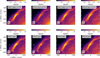 |
Fig. C.1 Comparison between the original IRAC images with the result of point-source subtraction. |
Star subtraction was performed using StarXTerminator3, an AI-based tool that employs neural networks to remove stellar sources from astronomical images. This tool was used as a plug-in within the PixInsight4 image-processing platform. To assess whether the subtraction introduced any bias, we masked the locations of the stars and correlated the star-subtracted template with the original image, finding a correlation slope of unity, which indicates that the subtraction is robust. An example comparison of the result of point-source subtraction is shown in Fig. C.1.
All Tables
Broad-band SEDs for selected regions, defined by the Band 1 fields they comprise.
All Figures
|
Fig. 1 ALMA Band 1 continuum imaging of the ρ Oph W filament. Each image is shown in linear stretch, and x- and y- axis are offset along RA and Dec from J2000 16:25:57.0 −24:20:48.0. (a) Restored image, in natural weighting, after point-source subtraction, with a beam of 8".696×6".436/-86deg (see text), and a noise of 5.55 μJy beam−1. (b) Same as panel a, but before point-source subtraction. The three bright point sources are the young stellar objects SR 4 near the centre, ISO-Oph-17 to the east, and DoAr 21 to the south. The cyan circles are centred on the phase directions of each field and their radii correspond to half the radius of the first Airy null (corresponding to a primary beam attenuation of ~0.34). (c) Deconvolved model image, Im, after point-source subtraction and with 1"2 pixels. |
| In the text | |
|
Fig. 2 Point source fits to DoAr 21, over individual interferometer scans, each ~ 10 min long. The top and bottom rows respectively record spectral index, α, and flux density, Fν, at the reference frequency of 40.15 GHz. The x-axis gives the Julian date, expressed in days from the start of the observations. |
| In the text | |
|
Fig. 3 Flux densities for DoAr 21, on 11-Mar-2024, extracted over 120-channel averages. The black line is the best fit point-source model from Table 2. Spectral windows are plotted in alternating colours. |
| In the text | |
|
Fig. 4 Flux densities for SR4, extracted over 120-channel averages. The black line is the best fit point-source model from Table 2. Spectral windows are plotted in alternating colours. |
| In the text | |
|
Fig. 5 Spectrum of the diffuse emission from ρ Oph W, as estimated with the cross-correlation slope, aν. The black line is the best-fit powerlaw spectrum, with spectral index indicated in the legends. Plots a-c correspond to spectra extracted over different parts of the mosaic, as indicated in each plot. Field IDs follow from Fig. 1. Spectral windows are plotted in alternating colours. |
| In the text | |
|
Fig. 6 Radio-IR linear regression in real and imaginary parts, with Band 1 visibilities on the x-axis, and simulated IRAC 3.6 μm visibilities on the y-axis. Axis units are given in Jy. Only data corresponding to uv-radii shorter than 2606λ have been selected. The green line corresponds to the best fit linear regression. |
| In the text | |
|
Fig. 7 Radio-IR slopes (in a) and Pearson r coefficient (in b) as a function of baseline length. The domain in uv-radius has been truncated at the maximum value for which the uncertainties become larger than a third of the reported values. |
| In the text | |
|
Fig. 8 Comparison of the ALMA Band 1 with IR templates. Insets highlight the compact EME source at J2000 RA 16:25:54.154, Dec −24:19:52.5. The blue contour traces the Band 1 image from Fig. 1a at 80% peak. (a) Band 1 deconvolved image (same as Fig. 1c, but with λ = 0.1 for comparison). (b-e) IRAC images, with 1″ pixels, and before point-source subtraction. (f) Restored Band 1 image (same as Fig. 1a, but with λ = 0.1). (g-j) Restorations of the IRAC simulations, after point-source subtraction, scaling by aIR, and addition of thermal noise, as in the Band 1 data. (k-o) Herschel images. |
| In the text | |
|
Fig. 9 Comparison of the 17.5 GHz (in a) and 20.2 GHz (in b) ATCA mosaics (from Casassus et al. 2021b) with the ALMA Band 1 pointings. The Band 1 restored image from Fig. 1a is overlaid in a single contour at 60% peak intensity. |
| In the text | |
|
Fig. 10 Power S(δb) across a continuous range of combs with line intervals ∆ν. The top panel is for the raw spectral resolution, and the lower panel uses a five-channel average. Uncertainties are shown as vertical ±1σ error bars in blue (with total length of 2σ), and are offset to zero for clarity. |
| In the text | |
|
Fig. 11 Uncertainty on the projected power in a continuous range of combs with line intervals ∆ν. |
| In the text | |
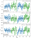 |
Fig. A.1 Same as Fig. 5, but for the IRAC 3.6 μm simulation. |
| In the text | |
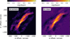 |
Fig. B.1 Comparison between gpu-uvmem (in a), same as Fig. 1a) and tclean reconstructions (in b). |
| In the text | |
|
Fig. C.1 Comparison between the original IRAC images with the result of point-source subtraction. |
| In the text | |
Current usage metrics show cumulative count of Article Views (full-text article views including HTML views, PDF and ePub downloads, according to the available data) and Abstracts Views on Vision4Press platform.
Data correspond to usage on the plateform after 2015. The current usage metrics is available 48-96 hours after online publication and is updated daily on week days.
Initial download of the metrics may take a while.