| Issue |
A&A
Volume 707, March 2026
|
|
|---|---|---|
| Article Number | A112 | |
| Number of page(s) | 16 | |
| Section | Extragalactic astronomy | |
| DOI | https://doi.org/10.1051/0004-6361/202558029 | |
| Published online | 02 March 2026 | |
EDGE-INFERNO: How chemical enrichment assumptions impact the individual stars of a simulated ultra-faint dwarf galaxy
1
Department of Astrophysics, American Museum of Natural History 200 Central Park West New York NY 10024, USA
2
Department of Physics, University of Bath Claverton Down Bath BA2 7AY, UK
3
Centre for Astrophysics Research, University of Hertfordshire Hatfield AL10 9AB, UK
4
University of Surrey, Physics Department, Guildford GU2 7XH, UK
5
Lund Observatory, Division of Astrophysics, Department of Physics, Lund University Box 43 SE-221 00 Lund, Sweden
6
Department of Astronomy & Astrophysics, University of Chicago, 5640 S Ellis Ave Chicago IL 60637, USA
7
Kavli Institute for Cosmological Physics, University of Chicago Chicago IL 60637, USA
8
NSF-Simons AI Institute for the Sky (SkAI), 172 E. Chestnut St. Chicago IL 60611, USA
9
Department of Astronomy, Columbia University, New York NY 10027, USA
10
Center for Astrophysics | Harvard & Smithsonian Cambridge MA 02138, USA
★ Corresponding author: This email address is being protected from spambots. You need JavaScript enabled to view it.
Received:
7
November
2025
Accepted:
26
January
2026
Abstract
The chemical abundances of stars in galaxies are a fossil record of the star formation and stellar evolution processes that regulate galaxy formation, including the stellar initial mass function, the fraction and timing of type Ia supernovae (SNeIa), and nucleosynthesis inside massive stars. In this paper, we systematically explore uncertainties associated with modeling chemical enrichment in dwarf galaxies. We repeatedly simulate a single EDGE-INFERNO dwarf (M★ ≈ 105 M⊙), varying the chemical yields of massive stars, the timing and yields of SNeIa, and the intrinsic stochasticity that arises from sampling individual stars and galaxy formation chaoticity. All simulations are high-resolution (3.6 pc), cosmological zoom-in hydrodynamical simulations that track the stellar evolution of all individual stars with masses of > 0.5 M⊙. We find that SNeIa make significant contributions to the iron content of low-mass, reionization-limited galaxies, with possible variations in mean abundance ratios and [Fe/H] related to minor changes in their evolutionary timescales. In contrast, different massive star yields, accounting (or not) for stellar rotation, result in mean abundance variations comparable to those arising from stochasticity, with the possible exception of extremely rapidly rotating stars. Nonetheless, massive stars significantly affect the shape of abundance trends with [Fe/H], for example, through the existence (or not) of a bimodality in the [X/Fe]–[Fe/H] planes, particularly in [Al/Fe]. Finally, we find that the variance arising from random sampling severely limits the interpretation of single galaxies. Our analysis showcases the power of star-by-star cosmological models to unpick how both systematic uncertainties (e.g., assumptions in low-metallicity chemical enrichment) and statistical uncertainties (e.g., averaging over enough galaxies and stars within a galaxy) affect the interpretation of chemical observables in ultra-faint dwarf galaxies.
Key words: galaxies: abundances / galaxies: dwarf / galaxies: formation
© The Authors 2026
 Open Access article, published by EDP Sciences, under the terms of the Creative Commons Attribution License (https://creativecommons.org/licenses/by/4.0), which permits unrestricted use, distribution, and reproduction in any medium, provided the original work is properly cited.
This article is published in open access under the Subscribe to Open model. This email address is being protected from spambots. You need JavaScript enabled to view it. to support open access publication.
1. Introduction
The faintest dwarf galaxies live in such shallow gravitational potential wells that they are expected to see their star formation histories abruptly suppressed at high redshift by reionization (Efstathiou 1992; Shapiro et al. 1994; Gnedin 2000; Bullock et al. 2000; Benson et al. 2002b,a; Somerville 2002). The population of ultra-faint dwarfs (UFDs; MV ≳ −7.75; L ≤ 105 L⊙; see Simon 2019 for a review), with most of their stars formed at z ≥ 4 (Brown et al. 2014; Weisz et al. 2014; Savino et al. 2023, 2025; Durbin et al. 2025), is a natural place to study such low-mass, reionization-limited galaxies.
In particular, the chemical elements locked in the photosphere of low-mass, long-lived stars in these dwarfs encode a fossil record of star formation events at z ≥ 4. Such chemical abundances can often be linked to specific sites of nucleosynthesis (Tinsley 1980; Timmes et al. 1995; Matteucci 2001; see also Maiolino & Mannucci 2019; Kobayashi et al. 2020a for recent reviews), in turn providing us with a unique window into star formation, stellar evolution, and nucleosynthesis processes that are hard to probe directly. Furthermore, measurements of chemical abundances in stars within faint dwarfs have been steadily increasing (see Pace 2025, for recently compiled data), in both [Fe/H] measurements (e.g., Muñoz et al. 2006; Martin et al. 2007; Simon & Geha 2007; Fu et al. 2023; Luna et al. 2025; Sandford et al. 2025) and other abundance ratios (e.g., Kirby et al. 2009; Frebel et al. 2010; Norris et al. 2010; Vargas et al. 2013; Ji et al. 2020; Skúladóttir et al. 2017, 2024).
These measurements have strongly established that the positive correlation between galaxy luminosity and stellar [Fe/H] (closely related to the stellar mass–metallicity relation) extends well into the regime of faint galaxies (Simon & Geha 2007; Kirby et al. 2013; Read et al. 2017), albeit with a possible flattening and/or increased scatter at V-band magnitude MV ≳ −5.5 (see, e.g., Simon 2019; Fu et al. 2023). Both the slope, the normalization, the scatter, and the potential plateau in this relation are sensitive to the details of how stellar feedback drives outflows in shallow potential wells (Agertz et al. 2020; Rey et al. 2025b), to the stellar initial mass function (IMF, Prgomet et al. 2022), to the formation of the first metal-free Population (Pop.) III stars (Jeon et al. 2017; Gutcke et al. 2022; Sanati et al. 2023; Rey et al. 2025a), and to the specific galaxy growth history (Rey et al. 2019). As such, this relation is often used to compare and discriminate between different dwarf galaxy formation models (e.g., Go et al. 2025; Rey et al. 2025a,b; Wheeler et al. 2025).
Beyond the average iron content and its relation with stellar mass, one can also leverage the distribution of individual metals (hereafter metal distribution functions, MDFs), their relationship to one another in fractional abundances, and to [Fe/H] as a tracer of total metallicity. For example, a downturn in the [α/Fe]–[Fe/H] plane (where α represents one or the sum of, e.g., O, Mg, Si, Ca, and Ti) is usually interpreted as revealing the time at which SNeIa start contributing significantly to iron production compared to massive stars. Such a “knee” is detected in many, but not all, faint dwarfs (Frebel & Bromm 2012; Frebel et al. 2014; Hill et al. 2019; Chiti et al. 2023), which could be leveraged into constraints on star formation and feedback timescales (e.g., Kirby et al. 2019; Alexander & Vincenzo 2025; Ting & Ji 2025. Similarly, the shape of the [Fe/H] MDF can be modeled through semi-analytical models to determine the length of the star formation histories and the strength of outflows (e.g., Alexander et al. 2023; Sandford et al. 2024; Luna et al. 2025), while specific abundances in UFDs have been linked to properties of metal-free stars (e.g., Jeon et al. 2017; Rossi et al. 2021).
However, the interpretation of chemical abundance data in dwarf galaxies relies on our understanding of how enrichment from stars formed at z ≥ 4 is imprinted into present-day observables. Predictions of elemental abundances in simulations necessitate chemical yields associated with different nucleosynthesis sites. Deriving these yields is computationally expensive, and instead, models of galactic chemical evolution rely on pre-tabulated estimates (see, e.g., Côté et al. 2013, 2016; Kobayashi et al. 2020a; Buck et al. 2021, 2025), even for semi-analytical modeling (Kobayashi et al. 2020a; Yates et al. 2021; Spitoni et al. 2023). As such, pre-tabulated yields have been available for a long time and are frequently being updated. These are typically divided into different sources; for example, asymptotic giant branch (AGB) stars (e.g., Marigo 2001; Karakas 2010; Karakas & Lugaro 2016; Pignatari et al. 2016; Ritter et al. 2018), super-AGB and electron capture SNe (Siess 2010; Doherty et al. 2014a,b; Gil-Pons et al. 2022; Limongi et al. 2024, 2025), core-collapse SNe (CCSNe) and winds from massive stars (e.g., Raiteri et al. 1996; Portinari et al. 1998; François et al. 2004; Chieffi & Limongi 2004; Nomoto et al. 2013; Frischknecht et al. 2016; Pignatari et al. 2016; Limongi & Chieffi 2018; Ritter et al. 2018), SNeIa (e.g., Iwamoto et al. 1999; Thielemann et al. 2003; Seitenzahl et al. 2013), hypernovae (Umeda & Nomoto 2002; Umeda et al. 2002; Nomoto et al. 2013), and pair-instability SNe (Heger & Woosley 2002; Umeda & Nomoto 2002; Cooke & Madau 2014).
However, even when focusing on the same stellar types, yields carry significant systematic uncertainties (e.g., stellar rotation, magnetic field strength, nuclear reaction rates, and modeling of explosions, Romano et al. 2010; Seitenzahl et al. 2013; Côté et al. 2016; Philcox et al. 2018; Kobayashi et al. 2020b, often resulting in significant differences in the chemical content of galaxies (Buck et al. 2021). These uncertainties are amplified at the low metallicities of UFDs, for which few massive stars can be observed around the Milky Way to anchor stellar evolution tracks. Because of these uncertainties, there is a pressing need to explore their impact on predictions of the chemical content of dwarf galaxies and, as a result, the ability of the chemistry of UFDs to shed light on metal-free and metal-poor stellar evolutionary processes.
In this work, we conduct such a systematic and controlled exploration to quantify how the abundance ratio of a UFD responds to changes in chemical yields and chemical enrichment assumptions. We use high-resolution cosmological simulations to self-consistently follow the dark matter assembly, star formation, and chemical enrichment history of a single UFD.
All simulations use a detailed stellar feedback and enrichment model, INFERNO, which incorporates chemical ejecta star by star rather than relying on integrated stellar populations (Andersson et al. 2023, 2025). The model ties the release of selected elements to individual stars going through different stages of evolution, including winds from massive O and B-type stars on the main sequence, winds from stars on the giant branch, and SNe, both as a result of CCSNe and from binary evolution (SNeIa). For each source, nucleosynthesis yields in the ejecta were calculated using bilinear interpolation of pre-tabulated values obtained in the literature. The model is flexible, and any yields provided for the sources tracked in our model can be incorporated with only minor adjustments to the code base. With this tool at hand, we explore sets of commonly applied tables found in the literature (Pignatari et al. 2016; Ritter et al. 2018; Limongi & Chieffi 2018; Seitenzahl et al. 2013), aiming to test the robustness of abundance signatures, MDFs, and average [Fe/H] across assumptions.
We describe the numerical methods in Sect. 2, including our star-by-star enrichment model in 2.1 and the cosmological simulation setup in Sect. 2.2. We present the average iron content, MDFs, and abundances in 13 re-simulations of the same object in Sect. 3, varying the yields of massive stars, the parametrization and yields of SNeIa, and the compounded stochastic variance from sampling star formation and feedback using random number generators. We discuss our results and the limitations of our model in Sect. 4 and conclude in Sect. 5.
2. Methods
Our model works on a star-by-star basis. In this section we describe our treatment of stellar evolution and how stars interact with their surroundings through feedback in Sect. 2.1. We describe the numerical treatment of star formation, IMF sampling, stellar dynamics, and feedback injection in Sect. 2.2. The total mass loss for any source is based on look-up tables, described in Sect. 2.1.1.
2.1. Star-by-star chemical enrichment
The model approximates stellar evolution with a few important stellar phases. We omit proto-stellar evolution, starting stars on the main sequence for a duration calculated based on the mass and metallicity dependent fitting function by Raiteri et al. (1996). After the main sequence, we assume that stars between 8 and 25 M⊙ undergo CCSNe, while more massive stars directly collapse into a black hole (Janka 2012; Zapartas et al. 2021). Less massive stars instead spend a relatively short period as giants. This phase lasts until their envelope has been ejected, and only the core remains as a white dwarf.
Massive (≥8 M⊙) stars eject fast (∼1000 km s−1) winds while on the main sequence (Vink 2015). During this time, the mass loss rate is in the range of 10−8−10−6 M⊙ yr−1. In our model, the exact rate is determined by the total mass ejected during this phase, divided by the main-sequence lifetime. This is an approximation as winds from O and B-type stars ramp up significantly during the final stages of the main sequence. Therefore, winds from individual stars are overestimated at early times with our constant mass-loss rate, but underestimated at the end.
Low-mass stars inject slow (10 km s−1) winds in pulses with mass loss rates of 10−8−10−4 M⊙ yr−1 (Höfner & Olofsson 2018). In our model, we approximate these pulses by a constant rate, 10−5 M⊙ yr−1; this rate determines the duration of the wind from the total mass ejected. As with massive stars, the amount of ejecta is determined by yields (Sect. 2.1.1). With the yields applied in this work, stars match the initial-final mass relation for these types of stars (Cummings et al. 2016).
To model the rate of SNeIa, we stochastically sampled a discrete number of events from a delay-time distribution at each timestep, Δt. The delay-time distribution is given by
![Mathematical equation: $$ \begin{aligned} n_{\rm Ia}=I_{\rm Ia}\, M_{\rm sf}\,\left[\frac{t}{\mathrm{Gyr}}\right]^{-1.12}\Delta t,\quad t>t_{\rm Ia}, \end{aligned} $$](/articles/aa/full_html/2026/03/aa58029-25/aa58029-25-eq1.gif) (1)
(1)
where IIa = 2.6 × 10⁻¹³ yr−1 M⊙−1 is a normalization to the observed field SNIa rate (Maoz & Graur 2017), and Msf ≲ 500 M⊙ is the total mass used to sample stars at each star formation event. The delay-time, tIa, parametrizes the time after star formation before which any SNeIa can occur. Our fiducial choice is tIa = 38 Myr, motivated by the main-sequence lifetime of an ONe white dwarf progenitor. We vary this parameter later, since the exact progenitors of SNeIa are uncertain and this timescale can vary across the range ≈38 − 400 Myr (Maoz & Graur 2017).
2.1.1. Element-by-element yields
The total and element-by-element mass loss from stars at different stages of stellar evolution is determined through bilinear interpolation of tabulated yields. While the method allows for the tracking of any element in the provided yield table, we limit this work to exploring C, N, O, Mg, Al, Si, and Fe. Briefly summarized: C and N are ejected from stars of different masses on the AGB (resulting in different timescales for enrichment); O, Mg, and Si are primarily produced in CCSN and trace chemical enrichment on 0.1 − 1 Gyr timescales when measured relative to Fe; Al production is sensitive to the amount of C in the core after He burning, and therefore depends on stellar evolution modeling. As in previous EDGE models, we define total metallicity from MZ = 2.09 MO + 1.06 MFe (Agertz et al. 2020)1. For stars with properties outside the tabulated ranges, we allowed the method to extrapolate, while ensuring that mass loss did not exceed 90% of the star’s initial mass. Tables are divided into different types of sources: mass loss from 0.5 to 8.0 M⊙ stars after the main sequence (henceforth referred to as AGB ejecta); mass loss from 8.0 to 100 M⊙ mass stars during the main sequence (henceforth referred to as winds); explosive ejections when 8.0 − 25 M⊙ undergo CCSNe; explosive ejections for SNeIa.
In this work, all simulations use the same model for AGB ejecta from NUGRID (Pignatari et al. 2016; Ritter et al. 2018), tabulated in eight bins in stellar mass between 1.0 and 7.0 M⊙ and five bins in metallicities 0.005 − 1.0 Z⊙, where Z⊙ = 0.02. For winds and CCSN, we tested two sets of yield tables from NUGRID (Pignatari et al. 2016; Ritter et al. 2018) and three sets of yield tables from Limongi & Chieffi (2018, LC18 hereafter). For NUGRID, the yield sets are distinguished by rapid and delayed explosion mechanisms for CCSN. The rapid explosion mechanism limits the time (250 ms) allowed for kinetic energy to be generated from neutrino pressure to overcome the kinetic energy of in-falling material (Fryer et al. 2012). The delay allows for an explosion if this criterion is reached later. Each NUGRID model is tabulated in four bins in stellar mass between 12 and 25 M⊙ and with the same metallicity bins as for AGB ejecta. The yields from LC18 provide tables for rotation velocities 0, 150, and 300 km s−1, tabulated in four metallicity bins between 0.0016 and 0.675 Z⊙ and in nine bins between stellar masses 13 − 120 M⊙. In addition to testing each rotation model separately, we included a simulation in which each star was assigned rotation at birth based on randomly sampling the rotation distributions from Prantzos et al. (2018). This rotation was then used to determine which of the yield tables from LC18 to use on a star-by-star basis.
For SNeIa, we used yields from detonation models of Chandrasekhar-mass white dwarfs with equal initial mass in carbon and oxygen (Seitenzahl et al. 2013). We used their model N100, which is provided in four different metallicities covering the range 0.0065 − 0.65 Z⊙. The metallicity dependence is weak, and in most of our models we used only the highest-metallicity bin for simplicity. We included one simulation where the yields are interpolated in metallicity.
2.1.2. Enrichment from a single stellar population
We show the cumulative mass ejected of tracked elements and total metallicity (Z) from the studied yields models in Fig. 1. In this example, each model is evolved for 500 M⊙ of stars that are formed instantaneously (i.e., the behavior of each star formation event, later described in Sect. 2.2). Except for Fe and, in some models, N, the majority of mass in each element, as well as total metallicity, originates from CCSNe when summed over 13.8 Gyr, regardless of model. Fe production is dominated by SNIa, albeit only after ∼1 Gyr of evolution.
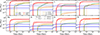 |
Fig. 1. Average cumulative mass of different elements (and total metallicity Z) injected by a mono-age population with mass 500 M⊙. Colors indicate different sources as labeled in the legend of the upper left panel. Except for SNIa, filled lines show the yields from NUGRID, while dashed lines show those from Limongi & Chieffi (2018) with different models (0, 150, 300 km s−1) shown with thicker lines for increasing rotation velocity. For SNIa, the filled (dashed) line shows the result with a delay time of 38 Myr (100 Myr). |
Yields from winds are relatively low compared to CCSN; however, the enrichment starts right after star formation. This makes self-enrichment in star-forming regions and stellar clusters possible (local star formation is typically self-quenched on timescales ≲10 Myr, Andersson et al. 2024). Comparing NUGRID and LC18, the latter has significantly stronger winds at high stellar rotation (at no rotation, C, N, and O yields are lower in LC18 and comparable to NUGRID for heavier elements).
Similarly, CCSN models with rotation significantly enhance the production of N, O, Al, and Si (and result in a small enhancement in C). Except for N (which is decreased) and Al (which is increased), 0 km/s rotation yields for CCSN in LC18 were comparable to those in NUGRID. The total CCSN Fe production is similar between LC18 and NUGRID; however, the evolution differs in the period when CCSNe are exploding (8 − 40 Myr). Very massive stars produce more Fe in all models from LC18 (early rapid increase in Fe); however, NUGRID quickly catches up when stars around 8 − 12 M⊙ start exploding. This is partly due to extrapolation of the yield table (see Sect. 2.1.1 for further details about the extrapolation method), which only extends to 12 M⊙; therefore, the Fe yields in our implementation of the NUGRID yields are likely overestimated (see also discussion in Rey et al. 2025b).
Compared with other sources (except winds), AGB stars produce large amounts of C and N (note that compared to SNIa, Z production is comparable, and O production is higher). Importantly, AGB stars behave similarly to SNeIa, producing enriched material over several gigayears, particularly C and O.
The SNeIa are important sources of Si, Fe, and Z, although we note that O production is similar to that of AGB stars. While SNeIa typically occur on longer timescales, each event produces a large amount of material. Therefore, on average, SNIa enrichment is reasonably high in terms of mass in the first few hundred million years. Because of this, the assumption of tIa is important and plays a significant role in the early enrichment of elements originating from SNIa. We exemplify the effect of sampling discrete SNeIa in Fig. 2, showing the tracks representing the median and 68th percentiles of a 500 M⊙ stellar population, assuming tIa = 38 Myr. On average, one such population produces 0.85 SNeIa in a 13.8 Gyr, while the same number for our model assuming tIa = 100 Myr is 0.64. For our simulations, the dwarf galaxies experience approximately 190 and 130 SNeIa for a tIa of 38 Myr and 100 Myr, respectively. Furthermore, Fig. 2 shows that only 50% of 500 M⊙ populations produce a SNIa within the first 4 Gyr; however, 16% produce one within the first ≈100 Myr. For comparison, in models with tIa = 100 Myr, 16% of 500 M⊙ populations produce one within the first ≈300 Myr.
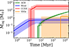 |
Fig. 2. Median total mass loss as a function of time, with colored regions showing the 68 percentiles for 1000 samples of 500 M⊙ drawn from the IMF. This example uses the yields from NUGRID, and type Ia delay time of 38 Myr, but the scatter in injected mass at a given time is similar regardless of the model. Note that the large scatter in SNIa arises because of forcing discrete events for a small amount of stellar mass. |
All feedback (including the ejection of chemical elements) is determined on a star-by-star basis; therefore, feedback is inherently stochastic from sampling of the IMF and timing of events. This implies that each quanta of 500 M⊙ produces different amounts of ejecta, as was discussed for SNeIa in the previous paragraph. Figure 2 quantifies this scatter for other sources as well, showing the median and 68th percentiles of the cumulative mass loss as a function of time for one of our models. Noise sampling of the IMF generates factor-of-a-few changes in injected mass, comparable in scale to some of the differences between yield models. This, combined with other sources of stochasticity in galaxy formation modeling, motivates the quantification of stochastic effects in Sect. 3.
2.2. Numerical method and initial conditions
Our numerical framework built on a modified version of the adaptive mesh refinement (AMR) and N-body code RAMSES2 code (Teyssier 2002). The fluid equations were solved using a second-order unsplit Godunov method (HLLC) for the Riemann solver (Toro et al. 1994) with a MinMod slope limiter. Gravitational dynamics were treated via the Poisson equation using the multi-grid method (Guillet & Teyssier 2011), treating all stellar and dark matter as collisionless particles with mapping to the AMR grid by the cloud-in-cell particle-mesh method. We tracked the mass fraction of elements by advecting passive scalars, fi, in time, t, with the fluid flow following
 (2)
(2)
where ρ and v are the fluid density and velocity, respectively.
Gas cooling and heating are described in detail in Rey et al. (2020). In summary, we assume an ideal monoatomic gas with adiabatic index γ = 5/3, and limit temperatures to the range 1 − 109 K. Our routine accounts for hydrogen and helium thermochemistry assuming equilibrium conditions (Courty & Alimi 2004; Rosdahl et al. 2013) and metal line cooling based on CLOUDY (Ferland et al. 1998). In addition, we added photoionization and photo-heating rates from a UV background modified from Haardt & Madau (1996), including a suppression of these rates in dense, self-shielded gas (Aubert & Teyssier 2010; Rosdahl & Blaizot 2012). To account for the unresolved formation of Population III stars in our simulations, we seeded the zoom region with an oxygen fraction of 2 × 10⁻⁵. Early star formation is insensitive to the exact choice of this floor (Agertz et al. 2020), but the lack of metal-free star modeling will lead to spurious abundances at very low [X/Fe]. Out of caution, we removed stars with [Fe/H] < −4 in our analysis, as these might have abundances affected by enrichment from Pop. III stars (Jeon et al. 2017).
All simulations in this work start from the same initial conditions and employ a zoom-in refinement strategy to target the formation of a single galaxy in Λ cold dark matter cosmology. Our initial conditions were generated using GENETIC (Roth et al. 2016; Rey & Pontzen 2018; Stopyra et al. 2021). They assumed cosmological parameters from Planck Collaboration XVI (2014) and include targeted changes to the growth history using the “genetic modification” method (for more details, see Rey et al. 2019; Agertz et al. 2020; Andersson et al. 2025). The zoom-in region was defined to include all particles within two times the virial radius at z = 0, obtained beforehand from a 5123 dark matter only simulation (Rey et al. 2019, 2020). For simulations presented in this work, dark matter particles were given a mass of 940 M⊙ within the zoom-in region, and step-wise increased by factors of eight up to a mass of 2.5 × 10⁸ M⊙, using a buffer region of at least eight grids in width between each step3. Furthermore, the AMR grid was adapted from 7 to 25 levels of refinement (maximum resolution of 3.6 pc at z = 0) to keep the cell baryon (stars+gas) mass around 167 M⊙. Furthermore, refinement was set to maintain approximately eight dark matter particles per cell, which reduces discreteness effects (Romeo et al. 2008).
2.3. Star formation and feedback
Star formation, stellar evolution, and feedback were treated by the INFERNO model described in detail in Andersson et al. (2023). A star formation check was triggered when gas cells within the refinement region exceeded a density of ρ = 300 cm−3 if the gas was colder than 1000 K. In cells satisfying this criterion, we computed a star formation rate density of
 (3)
(3)
where tff is the free-fall time of the gas cell, and ϵff = 0.1 is an assumed star formation efficiency per free-fall time. The parametrization of our star formation recipe has been shown to successfully match key observables, both in EDGE (see, e.g., Rey et al. 2019; Agertz et al. 2020; Rey et al. 2025b) and INFERNO (Andersson et al. 2020, 2023, 2025) simulations. Based on the  , star formation is actualized in discrete quanta of Msf = 500 M⊙ using Poisson sampling.
At star formation, individual stars were sampled from the IMF by Kroupa (2001), given by
 (4)
(4)
with two intervals denoted with i between 0.08 and 100 M⊙ split at m0 = 0.5 M⊙. In Eq. (4), A is a normalizing constant, C0 = 1.0 and C1 = C0m0a1 − a0 are constants ensuring continuity, a0 = 1.3 below m0 and a1 = 2.3 above. To sample the IMF, the method from Sormani et al. (2017) was used, with the same implementation as in Andersson et al. (2020). Stars with mass below 0.5 M⊙ are agglomerated into a single particle, while more massive stars are spawned as individual particles.
Simulation labels and assumption variations.
All stars inherit the velocity of the gas cell from which they formed. In addition, individual stars are given small velocity perturbations from a normal distribution with standard deviation of 0.01 km s−1. These small perturbations are not to be confused with natal kicks resulting in walk- and runaway stars previously used with INFERNO (Andersson et al. 2020, 2021, 2023). To limit the uncertainty related to assumptions about fast-moving stars, we leave a study of these types of objects for future work.
As is detailed in Sect. 2.1, stellar evolution sets the time when stars inject mass, momentum, energy, and the chemical elements traced by scalar fields. All these quantities are injected into the nearest eight cells following the implementation of Agertz et al. (2013). When active, winds are injected continuously at constant velocity; the wind velocity during AGB is 10 km s−1, and 1000 km s−1 for massive (> 8 M⊙) main-sequence stars. The CCSNe locations were determined by individual stars; however, because we did not track binary evolution, SNIa explosions had positions traced by the unresolved stellar populations. For these explosions, stars inject 1051 erg of thermal energy and the corresponding momentum given the total mass ejected. For each explosion, we checked if the cooling radius was resolved by at least six cells. If this is not the case, the scheme injects the terminal momentum based on the Sedov-Taylor solution calibrated by Kim & Ostriker (2015). Our implementation has been shown to reproduce the total momentum and energy injection even at low resolution (Ohlin et al. 2019), and we note that < 10% of explosions are in the unresolved regime (see further discussion in Rey et al. 2025b).
A further description of the INFERNO model is provided in Andersson et al. (2023), including a presentation of the total mass, momentum, and energy budget. Furthermore, Andersson et al. (2023) found convergence for star formation and feedback at the resolution in this work, given our choices of parameters.
2.4. Suite of simulations
Our simulations are executed from the same initial conditions, applying different choices relevant to chemical evolution (see Fig. 1). The final halo mass (redshift z = 0) of this galaxy is M200 = 1.4 × 10⁹ M⊙, with M200 defined as the mass enclosed within the spherical radius r200 = 24 kpc, where the density is 200 times the cosmic critical density.
We then re-simulated this same object, changing the chemical enrichment parameters as summarized in Table 1. To summarize, we divided our experiments into different families: (1) two massive star yield sets from NUGRID; (2) four massive star yield sets from LC18 with different stellar rotation; (3) variations in SNIa delay times and yields; and (4) results from repeated simulations with the same chemical assumptions but for which the random seed for galaxy and star formation has been varied4.
Comparing (1) and (2) allows us to compare two state-of-the-art yields for massive stars available in the literature. (3) allows us to test the importance of SNIa and control the amount of iron without drastically affecting the abundances of light elements. Finally, galaxy formation and stellar abundances have several sources of intrinsic noise associated with them, from sampling the IMF in low-mass systems (e.g., Fig. 2) to the general chaoticity of galaxy formation (see, e.g., Genel et al. 2019; Keller et al. 2019; Pakmor et al. 2025). (4) allows us to quantify the intrinsic scatter in our predictions within a given model and provide a metric by which to establish the significance of observed shifts between models.
We show the cumulative stellar mass of all simulations in Fig. 3. As was expected, different models lead to slightly different star formation histories and stellar mass assemblies. However, differences between chemical enrichment variations are consistent with differences induced by pure stochasticity within a single model (e.g., top panel, blue lines). As a result, we conclude that the stellar mass assembly is consistent across all chemical enrichment models.
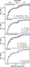 |
Fig. 3. Cumulative stellar mass as a function of stellar age (bottom axis) and redshift (top axis). Simulations are divided into the same groups as in Table 1, emphasizing the assumption that is varied in each panel (each panel is labeled in the top left corner). The top panel shows three simulations using different lines but the same color for the two different models. |
3. Results
3.1. The luminosity–[Fe/H] relation
Figure 4 shows the mean value of [Fe/H] as a function of the total V-band magnitude for all simulations presented in this work. They are contrasted with estimates from observed dwarf galaxies in the Local Volume marked by gray error bars. Data points for observed systems show MV and the associated upper and lower errors, while the [Fe/H] shows the spectroscopically determined values with errors indicating its dispersion. Note that vertical errors on the simulation data points also indicate [Fe/H] dispersion, not a measurement error. The data was obtained from the database by Pace (2025) and includes data from Carlin et al. (2009), Kirby et al. (2013), Martin et al. (2014), Kirby et al. (2015), Slater et al. (2015), Li et al. (2017), Simon (2019), Pace et al. (2020), Wojno et al. (2020), Kirby et al. (2020), Collins et al. (2021), Jenkins et al. (2021), Ji et al. (2021), Charles et al. (2023), Heiger et al. (2024), Kvasova et al. (2024), and Müller et al. (2025).
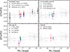 |
Fig. 4. Mean iron abundance, ⟨[Fe/H]⟩, as a function of total V-band magnitude, MV, for all simulations presented in this work, divided into four groups (see Table 1) for easier comparison. Top left: exploring the role of stochasticity by fixing the subgrid model to be NUGRID (delay) with tIa = 38 Myr (red) or LC18 with tIa = 100 Myr (blue) varying only the random number seed. This panel also includes the simulations from Andersson et al. (2025) in black. Top right: exploring the rotation models from LC18 (teal, green, and blue for 0, 150, and 300 km s−1, respectively), including one example with the rotation distribution from Prantzos et al. (2018, purple). All these models use tIa = 38 Myr. Lower left: testing different SNIa models, including 38 (green) and 100 Myr (blue) for tIa, one example without SNIa (purple), and one with metallicity-dependent SNIa yields (teal). All models use yields from LC18 for massive stars. Bottom right: comparing the NUGRID models with the delay (red) and rapid (blue) explosion triggers for CCSN, both with tIa = 38 Myr. These simulations use a model identical to NUGRID (delay), tIa = 38 Myr, but from different initial conditions. The error bars on the vertical axis indicate the dispersion in [Fe/H], calculated by taking the standard deviation of all stars in each galaxy. Gray error bars show values from dwarf galaxies in the Local Group Volume, taken from the database by Pace (2025). For these points, MV has error bars indicating upper and lower errors, while error bars on [Fe/H] indicate the dispersion. The dashed gray line shows the dwarf galaxy luminosity-[Fe/H] fit from Kirby et al. (2013). |
Starting from the top left panel, simulations with the same model but different random seeds evolve along the observed trend (Kirby et al. 2013), but retain a clear ordering in which the NUGRID (delay) model with tIa = 38 Myr always has higher ![Mathematical equation: $ \langle[\rm Fe/H]\rangle $](/articles/aa/full_html/2026/03/aa58029-25/aa58029-25-eq6.gif) . We can disentangle the origin of this difference by comparing variations in massive star yields (right column) and in SNIa assumptions (bottom left). Considering only the position in MV and mean [Fe/H], we find that different massive star yield tables cannot be distinguished from stochastic variations. The only potential exception is the extreme LC18 model, for which all stars are assumed to rotate at 300 km/s, which shows a mean [Fe/H] 0.3 dex below the relation (blue, upper right panel). But accounting for the full rotation distribution increases the average [Fe/H] closer to the average relation (dashed line). By contrast, SNeIa have a more systematic impact, whereby delaying and eventually removing SNIa results in a [Fe/H] that is 0.6 dex below the Kirby et al. (2013) relation. The systematic offset between stochastic re-simulations in our two models is thus readily attributed to their difference in SNeIa delay time distribution.
. We can disentangle the origin of this difference by comparing variations in massive star yields (right column) and in SNIa assumptions (bottom left). Considering only the position in MV and mean [Fe/H], we find that different massive star yield tables cannot be distinguished from stochastic variations. The only potential exception is the extreme LC18 model, for which all stars are assumed to rotate at 300 km/s, which shows a mean [Fe/H] 0.3 dex below the relation (blue, upper right panel). But accounting for the full rotation distribution increases the average [Fe/H] closer to the average relation (dashed line). By contrast, SNeIa have a more systematic impact, whereby delaying and eventually removing SNIa results in a [Fe/H] that is 0.6 dex below the Kirby et al. (2013) relation. The systematic offset between stochastic re-simulations in our two models is thus readily attributed to their difference in SNeIa delay time distribution.
Overall, we conclude that the position in MV and mean [Fe/H] is robust to the chemical enrichment assumptions tested, with our only simulation that can be ruled out being the model with no SNeIa at all. Our results also show that stochastic effects within a single or a couple of faint dwarf galaxies will make it extremely challenging to differentiate between chemical models based on the position in MV and mean [Fe/H] alone. To emphasize this point, we show the three different growth histories from Andersson et al. (2025) all with the NUGRID (delay) model with tIa = 38 Myr (black markers in the top left panel). Differences in mass assembly, star formation, and chemical enrichment histories at a fixed halo mass lead to larger shifts in average [Fe/H] (≈0.4 dex) than intrinsic stochasticity (≈0.2 dex), but comparable to SNeIa variations.
Nonetheless, chemical assumptions are likely to introduce systematic effects across the whole dwarf galaxy population and could be teased out through statistical modeling of populations (see e.g., Rey et al. 2025b for a visualization of this effect). Alternatively, a careful comparison between points in Fig. 4 reveals that the spread in [Fe/H] (vertical errors) is somewhat sensitive to the choice of yields, highlighting that more detailed chemical observables (e.g., MDFs) might provide additional sensitivity to chemical modeling. We focus on this in the next section.
3.2. Metal distribution functions
Figures 5 and 6 show MDFs quantified by [Fe/H] for our simulations. The bin width of 0.2 dex is comparable to the typical observational error. In addition, we show the combined MDF of all three simulations in both panels with black lines. The only robust difference is the systematic shift toward lower [Fe/H] when increasing tIa, as was already discussed in the previous section.
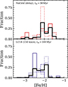 |
Fig. 5. MDF of [Fe/H] of six simulations used to estimate the stochastic variance, each displayed showing the fraction of stars in bins with size 0.2 dex, comparable to the typical errors on observed estimates of these quantities. The colored lines show individual simulations, each distinguished by different lines, while the black lines show the combined MDF of all simulations using the same model. The top row shows results from the NUGRID (delay) model with SNIa delay time of 38 Myr, and the bottom row shows results from the LC18 model with 150 km s−1 rotation and a delay time of 100 Myr for SNIa. Each row includes three simulations (different line styles) executed with a different seed for random number sampling. |
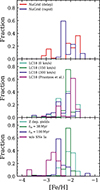 |
Fig. 6. MDF of [Fe/H] (as in Fig. 5) for the two models from NUGRID (top row), the four models including rotation (middle row), and the four different SNIa models (bottom row). See main text for details about each model. |
For completeness, we show MDFs of the different models in Fig. 6, dividing the groups outlined in Table 1 between the different panels. Overall, the MDFs are similar across the different model assumptions. Changing the massive-star yields or the stellar rotation rate produces only minor differences in the distributions. In some cases, the number and overall shape of peaks vary slightly, but these effects remain well within the stochastic variance. The only systematic change that is apparent, given typical measurement uncertainties, is the aforementioned shift toward lower [Fe/H] when delaying or removing SNeIa.
Note that we checked MDFs of other elements, including combinations of light elements ([α/Fe]), reaching similar conclusions. Instead, we turn to trends between relative abundances in the next section.
3.3. Relative abundances of individual elements
We turn to the abundances of individual elements, all presented relative to Fe in this work (i.e., [X/Fe] for element X) and shown as a function of [Fe/H]. Figure 7 shows the abundances of our simulations exploring random stochasticity within two models; NUGRID (delay), tIa = 38 Myr in red and LC18 (150 km/s), tIa = 100 Myr in blue. The different simulations can be distinguished by the difference in color shade. For all panels, we indicate the mean abundance of each simulation using a dashed line in the corresponding color.
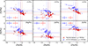 |
Fig. 7. Abundances relative to Fe as a function of [Fe/H] for different elements as indicated by the label in the upper right corner of each panel. The figure includes data from two different models in different shades of red and blue, as is indicated by the legend in the bottom right panel. For each model, different color shades present different simulations, varying only the random seed for IMF and SNIa sampling. The dashed vertical lines mark the mean value on the corresponding axis for each simulation. Included in the bottom (top) left of the top (bottom) row are colored error bars that show the total dispersion accounting for all stars in the three simulations of the corresponding color. |
In all cases, we observe the expected anticorrelation between [X/Fe] and [Fe/H]. As was already noted when studying Fig. 4, the mean [Fe/H] is higher for the NUGRID, tIa = 38 Myr runs due to the faster onset of SNeIa. As was expected, this also correlates with a systematically higher average [X/Fe] for all elements.
Furthermore, the star-by-star scatter obtained when combining all simulations with the same model is shown by errors in the bottom left of each panel. Note that the scatter averaged over a wide range of [Fe/H] does not necessarily quantify the variance at a given [Fe/H] (Mead et al. 2024), rather measuring the width of each element MDF (note the limitation that the total distribution is typically multi-peak). Comparing the two models, we note that [C/Fe] evolves more (larger scatter) in NUGRID (delay), tIa = 38 Myr, while [Al/Fe] and [Si/Fe] evolve less (lower scatter). The other elements show similar scatter in the two models. Except for [Al/Fe] in NUGRID (delay) and [Si/Fe] in both models, the star-by-star scatter is typically around 0.6 dex.
In addition to these broad trends in average abundances and scatter, element-by-element features appear that are related to the choice of yields. We discuss these in the next sections, but we note that outliers exist in almost all simulations, either with very high or very low [X/Fe] compared to their simulation average. We have tied these individual outlier stars to specific enrichment events that we shall report on in future work.
3.4. Abundance trends from different assumptions
Figures 8, 9, and 10 show the chemical abundances of individual stars in our three families of chemical assumptions. Focusing first on Fig. 8, we find that the two sets of NUGRID yields give highly consistent results for most elements that cannot be distinguished from differences introduced by stochasticity. As an example, the largest difference occurs in the mean [N/Fe] (≈ − 0.35 dex), which is comparable to stochastic shifts for [N/Fe] within the NUGRID model (Fig. 7, top center).
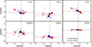 |
Fig. 8. Abundances (relative to iron) for the elements in our simulations (indicated in the top right of each panel), all as a function of iron abundance (relative hydrogen). The figure shows results from simulations that apply yields from NUGRID, including the delayed and rapid timing models for core-collapse explosion trigger (see main text for details). The mean value of all stars along each axis is shown by dashed lines in the color assigned to the model (see legend). |
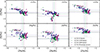 |
Fig. 9. Same as Fig. 8 but showing models with yields for massive stars from LC18 with different stellar rotation (see legend). In addition to single rotation models, we include a model that samples the rotation of each star at birth using the distribution from Prantzos et al. (2018) and applies the corresponding yield table. |
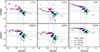 |
Fig. 10. Same as Fig. 8 but for models with different assumptions for SNIa, including two different time delays (tIa = 38 Myr and tIa = 100 Myr). In addition, we include one model without SNIa and one model in which yields (taken from Seitenzahl et al. 2013) are interpolated in metallicity (denoted Z dep. yields), but otherwise the same as the model with tIa = 38 Myr. All models take yields from LC18 with 150 km s−1 stellar rotation for massive stars. |
Similarly, Fig. 9 shows that the tables from LC18 are mostly consistent with each other and compared to intrinsic stochasticity. The largest shifts are observed for the extreme assumption that all massive stars rotate with velocities of 300 km s−1, driving an overproduction of N, O, Mg, Al, and Si. This overproduction is a direct result of the stellar evolution at increasing velocity (Fig. 1). For example, Mg and Al production is increased due to the decreased amount of C left after the He burning phase in the core as rotation velocities increase (Limongi & Chieffi 2018). Similarly, increasing stellar rotational velocity significantly augments the N output through early massive star winds (Fig. 1; see also Meynet & Maeder 2002; Chieffi & Limongi 2013).
Again, we find much more significant differences in the mean abundance ratios when varying assumptions related to SNeIa (Fig. 10). Delaying SNeIa from 38 to 100 Myr drives all element ratios up by up to ≥0.4 dex. Removing SNeIa entirely is even more dramatic, generating shifts up to ≈1 dex, much larger than stochastic effects. These increases are entirely driven by reducing the iron content across the board, rather than increasing the production of specific elements. These results emphasize the key role played by SNeIa in setting the chemistry of UFDs, despite their short star formation histories (≤2 Gyr).
Now focusing on broader trends beyond the mean and comparing families of simulations, we see markedly different behavior in [X/Fe]–[Fe/H] between NUGRID and LC18, most clearly visible in [C/Fe], [O/Fe], and [Si/Fe]. Comparing Figs. 8 and 9, we find that NUGRID models show a single relation between these elements and [Fe/H], while LC18 models appear bi-modal with a knee around [Fe/H] = −2.5, particularly in [Mg/Fe] and [Al/Fe]. This difference appears despite the same value for tIa and is robust compared to stochastic variance (see Fig. 7).
This knee is a well-established property of larger galaxies such as the Milky Way (Bensby et al. 2014; Bland-Hawthorn et al. 2019; Feuillet et al. 2019) and is usually interpreted as the point in the star formation history where SNeIa start contributing significantly to iron production. Our results corroborate these ideas, with the position for this knee around [Fe/H] = −2.5 not varying significantly with our assumptions for tIa, but the feature (and any stars with [Fe/H] > −2.5) disappearing entirely when SNeIa are removed (Fig. 10). Note that the relative insensitivity of the knee position to the Ia onset timing is to be expected, as the variations implemented in this work are small compared to the overall length of the star formation histories (≈1–2 Gyr).
A notable feature in the simulations without SNeIa (purple in Fig. 10) is the presence of two distinct trends at low [Fe/H] in both [C/Fe] and, to a lesser extent, [N/Fe]. At lower [C/Fe], the abundance ratios are set by the yields of massive stars, whereas the rising trend originates from the accumulation of AGB material in small halos prior to accretion onto the main progenitor. These halos also remain quiescent for extended periods between star formation. An AGB-driven formation for carbon-enhanced metal-poor stars has recently been suggested by Gil-Pons et al. (2025) and would require careful unpicking, since this population is often linked with pollution from the first stars (Klessen & Glover 2023). We shall provide a more detailed analysis of this feature in a forthcoming study (Andersson et al., in prep.).
4. Other sources of uncertainties yet to be tested
In this work, we test 13 different models of chemical enrichment with a high-resolution, star-by-star cosmological zoom simulation. Despite this extensive suite, the computational cost and limited complexity of INFERNO restricted the breadth of the parameter space exploration. In this section we highlight key areas that were not explored and that warrant further attention from future studies.
4.1. Additional sources of enrichment and the limitations of tabulated yields
We included variations of two sets of stellar feedback yields for massive stars, NUGRID (Pignatari et al. 2016; Ritter et al. 2018) and rotation-dependent yields from LC18. For low mass stars, we tested only yields from NUGRID, and for SNIa we applied yields from Seitenzahl et al. (2013). As is discussed in Sect. 1, this set of models is limited compared to the number of tabulated yields available in the literature.
Nonetheless, Buck et al. (2021) systematically tested a broader range of yields in higher-mass systems up to Milky-Way mass, concluding that the total metallicity and iron content are broadly insensitive to choice of massive star yields, but that individual elements and trends in [X/Fe]–[Fe/H] are. Our conclusions extend these findings to very low-mass systems, giving confidence that our conclusions remain robust even if a wider exploration of massive star yield models were to be considered.
Furthermore, the sources of chemical enrichment remain incomplete in our models. The most pressing limitation is the missing chemical yields for intermediate stellar masses. For low-mass stars (< 8 M⊙), we applied the tables from (Pignatari et al. 2016; Ritter et al. 2018), with data points between 1 and 7 M⊙. For higher-mass stars, these tables cover the mass range from 12 to 25 M⊙, while the tables from LC18 are in the range from 13 to 120 M⊙. This leaves a large range for extrapolation, a known issue for our simulations (Rey et al. 2025b). In fact, for the IMF applied here, this results in extrapolated yields for up to ≈50% (in terms of number) of all massive stars.
Yields for stars in the intermediate mass range (7 − 12 M⊙) are particularly challenging to derive due to their complex evolution (Doherty et al. 2015, 2017; Gil-Pons et al. 2018; Limongi et al. 2024). At the upper end of this mass range, these stars can result in electron-capture SNe, while stars at the lower end might result in exotic SNe (Foley et al. 2013). However, the exact mass range for electron-capture SNe is sensitive to metallicity and remains uncertain, although it is likely narrow (Doherty et al. 2015; Gil-Pons et al. 2018). Nonetheless, chemical yields in this mass range are available (e.g., Siess 2010; Doherty et al. 2014a,b; Gil-Pons et al. 2022; Limongi et al. 2025) and we are currently working on adding these to our model. In doing so, we shall address the effects of altering the boundary where the final stage of a star is a white dwarf.
Many other intriguing questions remain, in particular for the chemical signature in UFD galaxies. For example, because their low mass places them at the limit where metal retention is possible, dwarf galaxies can place constraints on the production of r-process elements, believed to originate from rare events such as exotic forms of SNe (collapsar and magnetorotational) and neutron-star mergers Ji et al. (2016), Côté et al. (2019), van de Voort et al. (2020), Tarumi et al. (2020). Furthermore, significant contributions from exotic forms of SNIa (e.g., Iax from sub-Chandrasekhar mass primogenitors) might be necessary to fully explain dwarf galaxy abundances Kobayashi et al. (2020b). Furthermore, a complete picture of chemical abundances most likely demands treatment of binary stars (Nguyen & Sills 2024), including common envelope overflow and novae, even in dwarf galaxies (Yates et al. 2024). These are some of the many sources that are yet to be fully explored with hydrodynamical models, providing promising venues for future work. We refer to Kobayashi et al. (2020a) for further discussion about additional sites of nucleosynthesis.
4.2. Zero-metallicity stars
In this paper, we do not consider the formation of stars from primordial gas; instead, we impose a homogeneous oxygen floor to represent this unresolved phase of chemical enrichment. In Appendix A we show that this floor has a minimal contribution to all oxygen abundances presented in this work.
Here, we also justify that the simplicity of this assumption is justified at the mass scale and environment we consider. Pop. III stars have been shown to make significant contributions to the mean iron content of UFDs when simulated in a proto-Milky-Way environment (e.g., Rey et al. 2025a), but much less in isolated field UFDs like we study here Jeon et al. (2017), Sanati et al. (2023). Furthermore, the chemical contribution from Pop. III stars is increasingly washed out as stellar masses increase toward the “massive” end of UFDs (105 M⊙), which we focus on in this work. As a result, it is unlikely that Pop. III physics would directly challenge the conclusions of this paper on the mean iron content.
However, a more detailed Pop. III model is likely necessary for a detailed analysis of the low-metallicity tail of the iron MDF ([Fe/H] ≤ −4.0; Jeon et al. 2017) and all abundance ratios at such metallicities. A first step could be to account for the fact that Pop. III enrichment affects multiple elements, rather than just oxygen, and implement an element-by-element floor calibrated on studies (such as Jaacks et al. 2018; Brauer et al. 2025). But a complete account of inhomogeneous pollution would require a dedicated implementation of the feedback and the chemical enrichment by individual Pop. III stars. This is a natural extension of INFERNO, which we plan to undertake in future work to enable studies similar to the one performed here, but varying key assumptions for Pop. III chemical enrichment in a lower-mass system.
Interestingly, while not modeled in our simulations, we note that signatures often attributed to Pop. III chemistry appear in our simulations. This includes metal-poor stars that are rich in carbon and nitrogen. We find several examples of this in Figs. 8, 9, and 7. Furthermore, the model without SNIa displays two separate trends in [C/Fe] and [N/Fe]: one at an almost constant ratio and one evolving toward a lower abundance with increasing [Fe/H]. We find that many of these signatures arise due to enrichment from AGB stars in low-mass proto-galaxies that are accreted later. Recent work has attributed such a signature to AGB enrichment (Gil-Pons et al. 2025). Fully explaining their origin is beyond the scope of this work, but it is planned for a future publication (Andersson et al., in prep.).
5. Conclusions
We present a suite of zoomed cosmological hydrodynamical simulations of a single UFD using an extension of the star-by-star INFERNO model. This extension generalizes the previous implementation to include detailed chemical ejecta as part of feedback from individual stars using any pre-tabulated yield table and combination of elements.
Leveraging this, we re-simulate the same dwarf galaxy 13 times, varying the input yield tables for massive stars, the yields and timescales for SNeIa, and quantifying the intrinsic stochasticity induced by IMF sampling and galaxy formation chaoticity within two chemical models. Our conclusions are:
-
SNIa are important contributors to the iron content of UFD stars. Delaying their onset from tIa = 38 Myr to tIa = 100 Myr consistently decreases [Fe/H] by ∼0.4 dex, and neglecting these explosions places galaxies well outside the luminosity–[Fe/H] relation.
-
Stochastic sampling of the IMF and feedback timescales introduces significant galaxy-to-galaxy scatter in stellar abundances. All elements in our simulations (C, N, O, Mg, Al, Si, and Fe) are susceptible to this effect.
-
Changing assumptions for massive star yields (e.g., including stellar rotation) result in quantitative but not qualitative differences in mean stellar abundances. These differences between models are of the same magnitude as those induced by pure stochasticity.
-
However, the choice of massive star yields affects the distribution of abundance trends when viewed as a function of [Fe/H]. In particular, we find that yields from LC18 produce bimodalities in the anticorrelation between light element abundances and [Fe/H], while others do not.
Our findings that mean dwarf galaxy abundances and the luminosity–[Fe/H] relation are converged with respect to different choices of yields extend the earlier findings from Buck et al. (2021) to much lower galaxy masses. This is particularly important for studies that aim to leverage the low-mass end of the luminosity–[Fe/H] relation to constrain the implementation of feedback and its ability to drive galactic winds (Wheeler et al. 2019; Agertz et al. 2020; Prgomet et al. 2022; Collins & Read 2022; Ibrahim & Kobayashi 2024; Rey et al. 2025b).
Our results also emphasize the importance of SNIa enrichment in UFDs. In fact, the largest shifts observed in mean abundances in our results are related to variations in SNeIa parameters. Despite the importance of SNeIa modeling in UFDs (see, e.g., Kirby et al. 2019; Alexander & Vincenzo 2025), these are not always considered in the context of galactic chemical enrichment of faint dwarfs due to the short star formation histories of these objects and the relative rarity of SNeIa per stellar mass (Go et al. 2025). However, even in reionization-limited UFDs, star formation histories extend over ≤2 Gyr, a timescale over which SNeIa easily play a role in enrichment. Furthermore, with a stellar mass of 105 M⊙, one expects ≈150 SNeIa explosions, a significant fraction of which are sampled within the first few hundred million years (see Fig. 2 and discussion in Sect. 2.2). These results strongly stress the importance of considering SNeIa when modeling the chemical enrichment of even UFDs.
Related to this, our simulations showcase a [α/Fe] downturn related to the time when SNeIa start contributing to Fe production. This occurs at [Fe/H] = −2.5 in our simulations, which is comparable to that often found in UFDs (Frebel et al. 2014; Chiti et al. 2023), although counterexamples exist Frebel & Bromm (2012). Perhaps unsurprisingly, our simulation with a galaxy of lower stellar mass (GM3: Latest, presented in Andersson et al. 2025, and included in our Fig. 4) does not show a clear downturn, further highlighting a dependence on stellar mass. We explore this in detail in Andersson et al. (in prep.). Simulations from Go et al. (2025) report that SNIa are unable to produce the downturn in [α/Fe] that we find at [Fe/H] ≈ −2.5. This could be a result of the lower stellar masses that they reported. However, we stress that the presence of a knee depends on the massive star yields applied in our models, warranting more exploration of whether the lack of a knee could be caused by their choice of CCSN yield set (Portinari et al. 1998).
Our results also emphasize the important role of stochasticity when interpreting the chemical content of a small number of dwarf galaxies. Different realizations of the same initial conditions and model can introduce differences comparable to those introduced by changing element yields. This challenge has been previously mentioned in the literature. Using simulations of dwarf galaxies from the FIRE model (Hopkins et al. 2014; see also Wheeler et al. 2019) with yields from NUGRID, Muley et al. (2021) found a significant increase in abundance scatter (particularly [α/Fe]) when including mass- and metallicity-dependent yields. The IMF sampling method also plays a role (Revaz et al. 2016), especially for extremely low-mass systems (Jeon & Ko 2024). Each of these stochastic events then compounds over time in a chaotic galaxy formation system, ultimately leading to different star formation and chemical enrichment histories (see also, Keller et al. 2019; Genel et al. 2019).
This is an important consideration for studies aiming to constrain low-metallicity chemical enrichment models with UFD data. For single systems, random sampling of stellar masses, feedback timing, and enrichment histories can produce outliers in abundances that differ by orders of magnitude, masking underlying physical correlations. These fluctuations will likely average out when considering large enough ensembles of galaxies, however, particularly since assumptions in chemical enrichment are likely to lead to systematic effects (e.g., delaying the onset of SNeIa would reduce the iron content of all dwarfs). Robust inference will require averaging over populations of dwarfs to overcome this intrinsic stochasticity. Furthermore, in addition to the galaxy-to-galaxy stochasticity, additional measurement noise is introduced by the limited number of individual stars per galaxy for which abundance measurements are made. This sampling noise can be as significant as some of the effects reported here, particularly in low-mass objects with few observable stars (Andersson et al. 2025).
Combined, these two factors underscore the need for a large sample of galaxies and large samples of stars per galaxy, a task that forthcoming spectroscopic surveys are currently undertaking (Simon 2019; Skúladóttir et al. 2023; Luna et al. 2025). Star-by-star models, which enable a direct connection to resolved star observations, combined with parameter explorations similar to the one performed in this study, are the perfect tools to estimate the necessary numbers of galaxies and stars per galaxy to obtain robust constraints on low-metallicity chemical enrichment assumptions.
Acknowledgments
We thank the anonymous reviewer for thoughtful comments, which improved the quality of this work. The authors thank Marco Limongi, Kira Lund, Stacy Kim, Pilar Gil Pons and Brian Schmidt for insightful discussions during the buildup of this work and comments on an earlier version of the manuscript. EPA and M-MML acknowledge support from NASA ATP grant 80NSSC24K0935 and NSF grant AST23-0795. JIR would like to acknowledge support from STFC grants ST/Y002865/1 and ST/Y002857/1. OA acknowledges support from the Knut and Alice Wallenberg Foundation, the Swedish National Space Agency (SNSA Dnr 2023-00164), and the LMK foundation. A.P.J. acknowledges support from the National Science Foundation under grant AST-2307599 and the Alfred P. Sloan Foundation. J.M. acknowledges support from the NSF Graduate Research Fellowship Program through grant DGE-2036197. K.B. is supported by an NSF Astronomy and Astrophysics Postdoctoral Fellowship under award AST-2303858. This work made extensive use of the dp191 and dp324 projects on the STFC-DiRAC ecosystem. This work was performed using the DiRAC Data Intensive service at Leicester, operated by the University of Leicester IT Services, which forms part of the STFC DiRAC HPC Facility (www.dirac.ac.uk). The equipment was funded by BEIS capital funding via STFC capital grants ST/K000373/1, ST/R002363/1, and STFC DiRAC Operations grant ST/R001014/1.
References
- Agertz, O., Kravtsov, A. V., Leitner, S. N., & Gnedin, N. Y. 2013, ApJ, 770, 25 [NASA ADS] [CrossRef] [Google Scholar]
- Agertz, O., Pontzen, A., Read, J. I., et al. 2020, MNRAS, 491, 1656 [Google Scholar]
- Alexander, R. K., & Vincenzo, F. 2025, MNRAS, 538, 1127 [Google Scholar]
- Alexander, R. K., Vincenzo, F., Ji, A. P., et al. 2023, MNRAS, 522, 5415 [Google Scholar]
- Andersson, E. P., Agertz, O., & Renaud, F. 2020, MNRAS, 494, 3328 [NASA ADS] [CrossRef] [Google Scholar]
- Andersson, E. P., Renaud, F., & Agertz, O. 2021, MNRAS, 502, L29 [NASA ADS] [CrossRef] [Google Scholar]
- Andersson, E. P., Agertz, O., Renaud, F., & Teyssier, R. 2023, MNRAS, 521, 2196 [NASA ADS] [CrossRef] [Google Scholar]
- Andersson, E. P., Mac Low, M.-M., Agertz, O., Renaud, F., & Li, H. 2024, A&A, 681, A28 [NASA ADS] [CrossRef] [EDP Sciences] [Google Scholar]
- Andersson, E. P., Rey, M. P., Pontzen, A., et al. 2025, ApJ, 978, 129 [Google Scholar]
- Aubert, D., & Teyssier, R. 2010, ApJ, 724, 244 [NASA ADS] [CrossRef] [Google Scholar]
- Bensby, T., Feltzing, S., & Oey, M. S. 2014, A&A, 562, A71 [NASA ADS] [CrossRef] [EDP Sciences] [Google Scholar]
- Benson, A. J., Frenk, C. S., Lacey, C. G., Baugh, C. M., & Cole, S. 2002a, MNRAS, 333, 177 [NASA ADS] [CrossRef] [Google Scholar]
- Benson, A. J., Lacey, C. G., Baugh, C. M., Cole, S., & Frenk, C. S. 2002b, MNRAS, 333, 156 [NASA ADS] [CrossRef] [Google Scholar]
- Bland-Hawthorn, J., Sharma, S., Tepper-Garcia, T., et al. 2019, MNRAS, 486, 1167 [NASA ADS] [CrossRef] [Google Scholar]
- Brauer, K., Emerick, A., Mead, J., et al. 2025, ApJ, 980, 41 [Google Scholar]
- Brown, T. M., Tumlinson, J., Geha, M., et al. 2014, ApJ, 796, 91 [NASA ADS] [CrossRef] [Google Scholar]
- Buck, T., Günes, B., Viterbo, G., Oliver, W. H., & Buder, S. 2025, A&A, 702, A184 [NASA ADS] [CrossRef] [EDP Sciences] [Google Scholar]
- Buck, T., Rybizki, J., Buder, S., et al. 2021, MNRAS, 508, 3365 [NASA ADS] [CrossRef] [Google Scholar]
- Bullock, J. S., Kravtsov, A. V., & Weinberg, D. H. 2000, ApJ, 539, 517 [CrossRef] [Google Scholar]
- Carlin, J. L., Grillmair, C. J., Muñoz, R. R., Nidever, D. L., & Majewski, S. R. 2009, ApJ, 702, L9 [NASA ADS] [CrossRef] [Google Scholar]
- Charles, E. J. E., Collins, M. L. M., Rich, R. M., et al. 2023, MNRAS, 521, 3527 [Google Scholar]
- Chieffi, A., & Limongi, M. 2004, ApJ, 608, 405 [NASA ADS] [CrossRef] [Google Scholar]
- Chieffi, A., & Limongi, M. 2013, ApJ, 764, 21 [Google Scholar]
- Chiti, A., Frebel, A., Ji, A. P., et al. 2023, AJ, 165, 55 [NASA ADS] [CrossRef] [Google Scholar]
- Collins, M. L. M., & Read, J. I. 2022, Nat. Astron., 6, 647 [NASA ADS] [CrossRef] [Google Scholar]
- Collins, M. L. M., Read, J. I., Ibata, R. A., et al. 2021, MNRAS, 505, 5686 [NASA ADS] [CrossRef] [Google Scholar]
- Cooke, R. J., & Madau, P. 2014, ApJ, 791, 116 [Google Scholar]
- Côté, B., Eichler, M., Arcones, A., et al. 2019, ApJ, 875, 106 [Google Scholar]
- Côté, B., Martel, H., & Drissen, L. 2013, ApJ, 777, 107 [Google Scholar]
- Côté, B., Ritter, C., O’Shea, B. W., et al. 2016, ApJ, 824, 82 [CrossRef] [Google Scholar]
- Courty, S., & Alimi, J. M. 2004, A&A, 416, 875 [NASA ADS] [CrossRef] [EDP Sciences] [Google Scholar]
- Cummings, J. D., Kalirai, J. S., Tremblay, P. E., & Ramirez-Ruiz, E. 2016, ApJ, 818, 84 [NASA ADS] [CrossRef] [Google Scholar]
- Doherty, C. L., Gil-Pons, P., Lau, H. H. B., Lattanzio, J. C., & Siess, L. 2014a, MNRAS, 437, 195 [Google Scholar]
- Doherty, C. L., Gil-Pons, P., Lau, H. H. B., et al. 2014b, MNRAS, 441, 582 [NASA ADS] [CrossRef] [Google Scholar]
- Doherty, C. L., Gil-Pons, P., Siess, L., Lattanzio, J. C., & Lau, H. H. B. 2015, MNRAS, 446, 2599 [Google Scholar]
- Doherty, C. L., Gil-Pons, P., Siess, L., & Lattanzio, J. C. 2017, PASA, 34, e056 [NASA ADS] [CrossRef] [Google Scholar]
- Durbin, M. J., Choi, Y., Savino, A., et al. 2025, ApJ, 992, 106 [Google Scholar]
- Efstathiou, G. 1992, MNRAS, 256, 43P [Google Scholar]
- Ferland, G. J., Korista, K. T., Verner, D. A., et al. 1998, PASP, 110, 761 [Google Scholar]
- Feuillet, D. K., Frankel, N., Lind, K., et al. 2019, MNRAS, 489, 1742 [Google Scholar]
- Foley, R. J., Challis, P. J., Chornock, R., et al. 2013, ApJ, 767, 57 [Google Scholar]
- François, P., Matteucci, F., Cayrel, R., et al. 2004, A&A, 421, 613 [NASA ADS] [CrossRef] [EDP Sciences] [Google Scholar]
- Frebel, A., & Bromm, V. 2012, ApJ, 759, 115 [Google Scholar]
- Frebel, A., Simon, J. D., Geha, M., & Willman, B. 2010, ApJ, 708, 560 [NASA ADS] [CrossRef] [Google Scholar]
- Frebel, A., Simon, J. D., & Kirby, E. N. 2014, ApJ, 786, 74 [NASA ADS] [CrossRef] [Google Scholar]
- Frischknecht, U., Hirschi, R., Pignatari, M., et al. 2016, MNRAS, 456, 1803 [Google Scholar]
- Fryer, C. L., Belczynski, K., Wiktorowicz, G., et al. 2012, ApJ, 749, 91 [Google Scholar]
- Fu, S. W., Weisz, D. R., Starkenburg, E., et al. 2023, ApJ, 958, 167 [Google Scholar]
- Genel, S., Bryan, G. L., Springel, V., et al. 2019, ApJ, 871, 21 [NASA ADS] [CrossRef] [Google Scholar]
- Gil-Pons, P., Doherty, C. L., Gutiérrez, J. L., et al. 2018, PASA, 35, e038 [NASA ADS] [CrossRef] [Google Scholar]
- Gil-Pons, P., Doherty, C. L., Campbell, S. W., & Gutiérrez, J. 2022, A&A, 668, A100 [NASA ADS] [CrossRef] [EDP Sciences] [Google Scholar]
- Gil-Pons, P., Campbell, S. W., Doherty, C. L., & Lugaro, M. 2025, A&A, 703, A107 [NASA ADS] [CrossRef] [EDP Sciences] [Google Scholar]
- Gnedin, N. Y. 2000, ApJ, 542, 535 [Google Scholar]
- Go, M., Jeon, M., Choi, Y., et al. 2025, ApJ, 986, 214 [Google Scholar]
- Guillet, T., & Teyssier, R. 2011, J. Comput. Phys., 230, 4756 [Google Scholar]
- Gutcke, T. A., Pakmor, R., Naab, T., & Springel, V. 2022, MNRAS, 513, 1372 [NASA ADS] [CrossRef] [Google Scholar]
- Haardt, F., & Madau, P. 1996, ApJ, 461, 20 [Google Scholar]
- Heger, A., & Woosley, S. E. 2002, ApJ, 567, 532 [Google Scholar]
- Heiger, M. E., Li, T. S., Pace, A. B., et al. 2024, ApJ, 961, 234 [Google Scholar]
- Hill, V., Skúladóttir, Á., Tolstoy, E., et al. 2019, A&A, 626, A15 [NASA ADS] [CrossRef] [EDP Sciences] [Google Scholar]
- Höfner, S., & Olofsson, H. 2018, A&ARv, 26, 1 [Google Scholar]
- Hopkins, P. F., Kereš, D., Oñorbe, J., et al. 2014, MNRAS, 445, 581 [NASA ADS] [CrossRef] [Google Scholar]
- Ibrahim, D., & Kobayashi, C. 2024, MNRAS, 527, 3276 [Google Scholar]
- Iwamoto, K., Brachwitz, F., Nomoto, K., et al. 1999, ApJS, 125, 439 [NASA ADS] [CrossRef] [Google Scholar]
- Jaacks, J., Thompson, R., Finkelstein, S. L., & Bromm, V. 2018, MNRAS, 475, 4396 [NASA ADS] [CrossRef] [Google Scholar]
- Janka, H.-T. 2012, Ann. Rev. Nucl. Part. Sci., 62, 407 [Google Scholar]
- Jenkins, S. A., Li, T. S., Pace, A. B., et al. 2021, ApJ, 920, 92 [NASA ADS] [CrossRef] [Google Scholar]
- Jeon, M., & Ko, M. 2024, MNRAS, submitted [arXiv:2411.17862] [Google Scholar]
- Jeon, M., Besla, G., & Bromm, V. 2017, ApJ, 848, 85 [NASA ADS] [CrossRef] [Google Scholar]
- Ji, A. P., Frebel, A., Chiti, A., & Simon, J. D. 2016, Nature, 531, 610 [NASA ADS] [CrossRef] [Google Scholar]
- Ji, A. P., Li, T. S., Simon, J. D., et al. 2020, ApJ, 889, 27 [NASA ADS] [CrossRef] [Google Scholar]
- Ji, A. P., Koposov, S. E., Li, T. S., et al. 2021, ApJ, 921, 32 [CrossRef] [Google Scholar]
- Karakas, A. I. 2010, MNRAS, 403, 1413 [NASA ADS] [CrossRef] [Google Scholar]
- Karakas, A. I., & Lugaro, M. 2016, ApJ, 825, 26 [NASA ADS] [CrossRef] [Google Scholar]
- Keller, B. W., Wadsley, J. W., Wang, L., & Kruijssen, J. M. D. 2019, MNRAS, 482, 2244 [NASA ADS] [CrossRef] [Google Scholar]
- Kim, C.-G., & Ostriker, E. C. 2015, ApJ, 802, 99 [NASA ADS] [CrossRef] [Google Scholar]
- Kirby, E. N., Guhathakurta, P., Bolte, M., Sneden, C., & Geha, M. C. 2009, ApJ, 705, 328 [NASA ADS] [CrossRef] [Google Scholar]
- Kirby, E. N., Cohen, J. G., Guhathakurta, P., et al. 2013, ApJ, 779, 102 [Google Scholar]
- Kirby, E. N., Simon, J. D., & Cohen, J. G. 2015, ApJ, 810, 56 [NASA ADS] [CrossRef] [Google Scholar]
- Kirby, E. N., Xie, J. L., Guo, R., et al. 2019, ApJ, 881, 45 [NASA ADS] [CrossRef] [Google Scholar]
- Kirby, E. N., Gilbert, K. M., Escala, I., et al. 2020, AJ, 159, 46 [NASA ADS] [CrossRef] [Google Scholar]
- Klessen, R. S., & Glover, S. C. O. 2023, ARA&A, 61, 65 [NASA ADS] [CrossRef] [Google Scholar]
- Kobayashi, C., Karakas, A. I., & Lugaro, M. 2020a, ApJ, 900, 179 [Google Scholar]
- Kobayashi, C., Leung, S.-C., & Nomoto, K. 2020b, ApJ, 895, 138 [CrossRef] [Google Scholar]
- Kroupa, P. 2001, MNRAS, 322, 231 [NASA ADS] [CrossRef] [Google Scholar]
- Kvasova, K. A., Kirby, E. N., & Beaton, R. L. 2024, ApJ, 972, 180 [Google Scholar]
- Li, T. S., Simon, J. D., Drlica-Wagner, A., et al. 2017, ApJ, 838, 8 [NASA ADS] [CrossRef] [Google Scholar]
- Limongi, M., & Chieffi, A. 2018, ApJS, 237, 13 [NASA ADS] [CrossRef] [Google Scholar]
- Limongi, M., Roberti, L., Chieffi, A., & Nomoto, K. 2024, ApJS, 270, 29 [NASA ADS] [CrossRef] [Google Scholar]
- Limongi, M., Roberti, L., Falla, A., Chieffi, A., & Nomoto, K. 2025, ApJS, 279, 41 [Google Scholar]
- Luna, A. M., Ji, A. P., Chiti, A., et al. 2025, Open J. Astrophys., 8, 47696 [Google Scholar]
- Maiolino, R., & Mannucci, F. 2019, A&ARv, 27, 3 [Google Scholar]
- Maoz, D., & Graur, O. 2017, ApJ, 848, 25 [Google Scholar]
- Marigo, P. 2001, A&A, 370, 194 [NASA ADS] [CrossRef] [EDP Sciences] [Google Scholar]
- Martin, N. F., Ibata, R. A., Chapman, S. C., Irwin, M., & Lewis, G. F. 2007, MNRAS, 380, 281 [CrossRef] [Google Scholar]
- Martin, N. F., Chambers, K. C., Collins, M. L. M., et al. 2014, ApJ, 793, L14 [NASA ADS] [CrossRef] [Google Scholar]
- Matteucci, F. 2001, The Chemical Evolution of the Galaxy (Dordrecht: Kluwer Academic Publishers), 253 [Google Scholar]
- Mead, J., Ness, M., Andersson, E., Griffith, E. J., & Horta, D. 2024, ApJ, 974, 186 [Google Scholar]
- Meynet, G., & Maeder, A. 2002, A&A, 390, 561 [NASA ADS] [CrossRef] [EDP Sciences] [Google Scholar]
- Muñoz, R. R., Carlin, J. L., Frinchaboy, P. M., et al. 2006, ApJ, 650, L51 [CrossRef] [Google Scholar]
- Muley, D. A., Wheeler, C. R., Hopkins, P. F., et al. 2021, MNRAS, 508, 508 [Google Scholar]
- Müller, O., Rejkuba, M., Fahrion, K., et al. 2025, A&A, 699, A207 [NASA ADS] [CrossRef] [EDP Sciences] [Google Scholar]
- Nguyen, M., & Sills, A. 2024, ApJ, 969, 18 [NASA ADS] [CrossRef] [Google Scholar]
- Nomoto, K., Kobayashi, C., & Tominaga, N. 2013, ARA&A, 51, 457 [CrossRef] [Google Scholar]
- Norris, J. E., Wyse, R. F. G., Gilmore, G., et al. 2010, ApJ, 723, 1632 [NASA ADS] [CrossRef] [Google Scholar]
- Ohlin, L., Renaud, F., & Agertz, O. 2019, MNRAS, 485, 3887 [Google Scholar]
- Pace, A. B. 2025, Open J. Astrophys., 8, 142 [Google Scholar]
- Pace, A. B., Kaplinghat, M., Kirby, E., et al. 2020, MNRAS, 495, 3022 [NASA ADS] [CrossRef] [Google Scholar]
- Pakmor, R., Bieri, R., Fragkoudi, F., et al. 2025, MNRAS, 543, 1761 [Google Scholar]
- Philcox, O., Rybizki, J., & Gutcke, T. A. 2018, ApJ, 861, 40 [Google Scholar]
- Pignatari, M., Herwig, F., Hirschi, R., et al. 2016, ApJS, 225, 24 [NASA ADS] [CrossRef] [Google Scholar]
- Planck Collaboration XVI. 2014, A&A, 571, A16 [NASA ADS] [CrossRef] [EDP Sciences] [Google Scholar]
- Portinari, L., Chiosi, C., & Bressan, A. 1998, A&A, 334, 505 [NASA ADS] [Google Scholar]
- Prantzos, N., Abia, C., Limongi, M., Chieffi, A., & Cristallo, S. 2018, MNRAS, 476, 3432 [Google Scholar]
- Prgomet, M., Rey, M. P., Andersson, E. P., et al. 2022, MNRAS, 513, 2326 [CrossRef] [Google Scholar]
- Raiteri, C. M., Villata, M., & Navarro, J. F. 1996, A&A, 315, 105 [NASA ADS] [Google Scholar]
- Read, J. I., Iorio, G., Agertz, O., & Fraternali, F. 2017, MNRAS, 467, 2019 [NASA ADS] [Google Scholar]
- Revaz, Y., Arnaudon, A., Nichols, M., Bonvin, V., & Jablonka, P. 2016, A&A, 588, A21 [NASA ADS] [CrossRef] [EDP Sciences] [Google Scholar]
- Rey, M. P., & Pontzen, A. 2018, MNRAS, 474, 45 [Google Scholar]
- Rey, M. P., Pontzen, A., Agertz, O., et al. 2019, ApJ, 886, L3 [Google Scholar]
- Rey, M. P., Pontzen, A., Agertz, O., et al. 2020, MNRAS, 497, 1508 [NASA ADS] [CrossRef] [Google Scholar]
- Rey, M. P., Katz, H., Cadiou, C., et al. 2025a, Open J. Astrophys., submitted [arXiv:2510.05232] [Google Scholar]
- Rey, M. P., Taylor, E., Gray, E. I., et al. 2025b, MNRAS, 541, 1195 [Google Scholar]
- Ritter, C., Herwig, F., Jones, S., et al. 2018, MNRAS, 480, 538 [NASA ADS] [CrossRef] [Google Scholar]
- Romano, D., Karakas, A. I., Tosi, M., & Matteucci, F. 2010, A&A, 522, A32 [NASA ADS] [CrossRef] [EDP Sciences] [Google Scholar]
- Romeo, A. B., Agertz, O., Moore, B., & Stadel, J. 2008, ApJ, 686, 1 [Google Scholar]
- Rosdahl, J., & Blaizot, J. 2012, MNRAS, 423, 344 [Google Scholar]
- Rosdahl, J., Blaizot, J., Aubert, D., Stranex, T., & Teyssier, R. 2013, MNRAS, 436, 2188 [Google Scholar]
- Rossi, M., Salvadori, S., & Skúladóttir, Á. 2021, MNRAS, 503, 6026 [NASA ADS] [CrossRef] [Google Scholar]
- Roth, N., Pontzen, A., & Peiris, H. V. 2016, MNRAS, 455, 974 [Google Scholar]
- Sanati, M., Jeanquartier, F., Revaz, Y., & Jablonka, P. 2023, A&A, 669, A94 [NASA ADS] [CrossRef] [EDP Sciences] [Google Scholar]
- Sandford, N. R., Weinberg, D. H., Weisz, D. R., & Fu, S. W. 2024, MNRAS, 530, 2315 [Google Scholar]
- Sandford, N. R., Li, T. S., Koposov, S. E., et al. 2025, ApJ, submitted [arXiv:2509.02546] [Google Scholar]
- Savino, A., Weisz, D. R., Skillman, E. D., et al. 2023, ApJ, 956, 86 [Google Scholar]
- Savino, A., Weisz, D. R., Dolphin, A. E., et al. 2025, ApJ, 979, 205 [Google Scholar]
- Seitenzahl, I. R., Ciaraldi-Schoolmann, F., Röpke, F. K., et al. 2013, MNRAS, 429, 1156 [NASA ADS] [CrossRef] [Google Scholar]
- Shapiro, P. R., Giroux, M. L., & Babul, A. 1994, ApJ, 427, 25 [Google Scholar]
- Siess, L. 2010, Mem. Soc. Astron. It., 81, 980 [Google Scholar]
- Simon, J. D. 2019, ARA&A, 57, 375 [NASA ADS] [CrossRef] [Google Scholar]
- Simon, J. D., & Geha, M. 2007, ApJ, 670, 313 [NASA ADS] [CrossRef] [Google Scholar]
- Skúladóttir, Á., Tolstoy, E., Salvadori, S., Hill, V., & Pettini, M. 2017, A&A, 606, A71 [NASA ADS] [CrossRef] [EDP Sciences] [Google Scholar]
- Skúladóttir, Á., Puls, A. A., Amarsi, A. M., et al. 2023, The Messenger, 190, 19 [Google Scholar]
- Skúladóttir, Á., Vanni, I., Salvadori, S., & Lucchesi, R. 2024, A&A, 681, A44 [NASA ADS] [CrossRef] [EDP Sciences] [Google Scholar]
- Slater, C. T., Bell, E. F., Martin, N. F., Tollerud, E. J., & Ho, N. 2015, ApJ, 806, 230 [Google Scholar]
- Somerville, R. S. 2002, ApJ, 572, L23 [NASA ADS] [CrossRef] [Google Scholar]
- Sormani, M. C., Treß, R. G., Klessen, R. S., & Glover, S. C. O. 2017, MNRAS, 466, 407 [NASA ADS] [CrossRef] [Google Scholar]
- Spitoni, E., Recio-Blanco, A., de Laverny, P., et al. 2023, A&A, 670, A109 [NASA ADS] [CrossRef] [EDP Sciences] [Google Scholar]
- Stopyra, S., Pontzen, A., Peiris, H., Roth, N., & Rey, M. P. 2021, ApJS, 252, 28 [CrossRef] [Google Scholar]
- Tarumi, Y., Yoshida, N., & Inoue, S. 2020, MNRAS, 494, 120 [Google Scholar]
- Teyssier, R. 2002, A&A, 385, 337 [CrossRef] [EDP Sciences] [Google Scholar]
- Thielemann, F. K., Argast, D., Brachwitz, F., et al. 2003, Nucl. Phys. A, 718, 139 [NASA ADS] [CrossRef] [Google Scholar]
- Timmes, F. X., Woosley, S. E., & Weaver, T. A. 1995, ApJS, 98, 617 [NASA ADS] [CrossRef] [Google Scholar]
- Ting, Y.-S., & Ji, A. 2025, Open J. Astrophys., 8, 7 [Google Scholar]
- Tinsley, B. M. 1980, Fund. Cosmic Phys., 5, 287 [Google Scholar]
- Toro, E. F., Spruce, M., & Speares, W. 1994, Shock Waves, 4, 25 [Google Scholar]
- Umeda, H., & Nomoto, K. 2002, ApJ, 565, 385 [Google Scholar]
- Umeda, H., Nomoto, K., Tsuru, T. G., & Matsumoto, H. 2002, ApJ, 578, 855 [Google Scholar]
- van de Voort, F., Pakmor, R., Grand, R. J. J., et al. 2020, MNRAS, 494, 4867 [NASA ADS] [CrossRef] [Google Scholar]
- Vargas, L. C., Geha, M., Kirby, E. N., & Simon, J. D. 2013, ApJ, 767, 134 [NASA ADS] [CrossRef] [Google Scholar]
- Vink, J. S. 2015, Very Massive Stars in the Local Universe (Cham: Springer), Astrophysics and Space Science Library, 412 [Google Scholar]
- Weisz, D. R., Dolphin, A. E., Skillman, E. D., et al. 2014, ApJ, 789, 147 [Google Scholar]
- Wheeler, C., Hopkins, P. F., Pace, A. B., et al. 2019, MNRAS, 490, 4447 [CrossRef] [Google Scholar]
- Wheeler, V., Kravtsov, A., Chiti, A., Katz, H., & Semenov, V. A. 2025, Open J. Astrophys., 8, 151 [Google Scholar]
- Wojno, J., Gilbert, K. M., Kirby, E. N., et al. 2020, ApJ, 895, 78 [Google Scholar]
- Yates, R. M., Henriques, B. M. B., Fu, J., et al. 2021, MNRAS, 503, 4474 [NASA ADS] [CrossRef] [Google Scholar]
- Yates, R. M., Hendriks, D., Vijayan, A. P., et al. 2024, MNRAS, 527, 6292 [Google Scholar]
- Zapartas, E., Renzo, M., Fragos, T., et al. 2021, A&A, 656, L19 [NASA ADS] [CrossRef] [EDP Sciences] [Google Scholar]
To calculate abundances relative to hydrogen, we assumed a primordial helium fraction (Y = 0.246) and calculated the hydrogen fraction X = (1 − Z)(1 − Y), i.e., assuming a constant Y at all Z. We leave to future work an explicit account of H and He enrichment.
Note that the multi-grid method used to calculate gravitational forces is well-suited to deal with the disparity between particle masses, which is important for systems with massive dark matter particles and low mass stars, which in our case can be 940 M⊙ dark matter particles interacting with 0.5 M⊙ star particles.
Our simulation code does not conserve the order of distributed arithmetic operations over time, so we simply re-run the same model on different core numbers to change the random seed.
Appendix A: Metallicity floor
To seed cooling in the gas at early times, we include a floor of 2 × 10⁻⁵ in the oxygen tracer of all our simulations. Oxygen is used to compute the metallicity passed to the cooling routine. In our simulations LC18 (150 km/s), tIa = 100 Myr, we included an additional oxygen tracer to test whether this initial value significantly affects the abundance that we derive. We compare the stellar abundances of these two tracers in Fig. A.1, showing three examples of the same model. As expected, the [O/Fe] is always higher in the tracer with an initial value. The difference is small for [O/Fe] excluding the floor between 0 and 1, but notably, there are some outliers at low [O/Fe], offset by almost 1 dex. These points correspond to metallicities around [Fe/H]≈ − 2. Notably, there is scatter between the simulations at these values. We also find that at the highest values, [O/Fe] diverges from the same tracer without the metal floor. In this case, there is a clear trend with [Fe/H]. The tracer without an initial value has a constant [O/Fe] value, which corresponds to that set by the ratio in the yield tables. The constant oxygen floor results in [O/Fe] shifting toward lower values as the relative amount of iron increases.
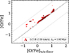 |
Fig. A.1. Comparison between the abundance of two identical tracers of oxygen, one of which (vertical axis) includes an initial floor of 2 × 10⁻⁵ to promote gas cooling at early times. The figure includes data from three simulations with different seed for random number generation but the same model; yields from LC18, 150 km s−1 for massive stars and tIa = 100 Myr). |
All Tables
All Figures
|
Fig. 1. Average cumulative mass of different elements (and total metallicity Z) injected by a mono-age population with mass 500 M⊙. Colors indicate different sources as labeled in the legend of the upper left panel. Except for SNIa, filled lines show the yields from NUGRID, while dashed lines show those from Limongi & Chieffi (2018) with different models (0, 150, 300 km s−1) shown with thicker lines for increasing rotation velocity. For SNIa, the filled (dashed) line shows the result with a delay time of 38 Myr (100 Myr). |
| In the text | |
|
Fig. 2. Median total mass loss as a function of time, with colored regions showing the 68 percentiles for 1000 samples of 500 M⊙ drawn from the IMF. This example uses the yields from NUGRID, and type Ia delay time of 38 Myr, but the scatter in injected mass at a given time is similar regardless of the model. Note that the large scatter in SNIa arises because of forcing discrete events for a small amount of stellar mass. |
| In the text | |
|
Fig. 3. Cumulative stellar mass as a function of stellar age (bottom axis) and redshift (top axis). Simulations are divided into the same groups as in Table 1, emphasizing the assumption that is varied in each panel (each panel is labeled in the top left corner). The top panel shows three simulations using different lines but the same color for the two different models. |
| In the text | |
|
Fig. 4. Mean iron abundance, ⟨[Fe/H]⟩, as a function of total V-band magnitude, MV, for all simulations presented in this work, divided into four groups (see Table 1) for easier comparison. Top left: exploring the role of stochasticity by fixing the subgrid model to be NUGRID (delay) with tIa = 38 Myr (red) or LC18 with tIa = 100 Myr (blue) varying only the random number seed. This panel also includes the simulations from Andersson et al. (2025) in black. Top right: exploring the rotation models from LC18 (teal, green, and blue for 0, 150, and 300 km s−1, respectively), including one example with the rotation distribution from Prantzos et al. (2018, purple). All these models use tIa = 38 Myr. Lower left: testing different SNIa models, including 38 (green) and 100 Myr (blue) for tIa, one example without SNIa (purple), and one with metallicity-dependent SNIa yields (teal). All models use yields from LC18 for massive stars. Bottom right: comparing the NUGRID models with the delay (red) and rapid (blue) explosion triggers for CCSN, both with tIa = 38 Myr. These simulations use a model identical to NUGRID (delay), tIa = 38 Myr, but from different initial conditions. The error bars on the vertical axis indicate the dispersion in [Fe/H], calculated by taking the standard deviation of all stars in each galaxy. Gray error bars show values from dwarf galaxies in the Local Group Volume, taken from the database by Pace (2025). For these points, MV has error bars indicating upper and lower errors, while error bars on [Fe/H] indicate the dispersion. The dashed gray line shows the dwarf galaxy luminosity-[Fe/H] fit from Kirby et al. (2013). |
| In the text | |
|
Fig. 5. MDF of [Fe/H] of six simulations used to estimate the stochastic variance, each displayed showing the fraction of stars in bins with size 0.2 dex, comparable to the typical errors on observed estimates of these quantities. The colored lines show individual simulations, each distinguished by different lines, while the black lines show the combined MDF of all simulations using the same model. The top row shows results from the NUGRID (delay) model with SNIa delay time of 38 Myr, and the bottom row shows results from the LC18 model with 150 km s−1 rotation and a delay time of 100 Myr for SNIa. Each row includes three simulations (different line styles) executed with a different seed for random number sampling. |
| In the text | |
|
Fig. 6. MDF of [Fe/H] (as in Fig. 5) for the two models from NUGRID (top row), the four models including rotation (middle row), and the four different SNIa models (bottom row). See main text for details about each model. |
| In the text | |
|
Fig. 7. Abundances relative to Fe as a function of [Fe/H] for different elements as indicated by the label in the upper right corner of each panel. The figure includes data from two different models in different shades of red and blue, as is indicated by the legend in the bottom right panel. For each model, different color shades present different simulations, varying only the random seed for IMF and SNIa sampling. The dashed vertical lines mark the mean value on the corresponding axis for each simulation. Included in the bottom (top) left of the top (bottom) row are colored error bars that show the total dispersion accounting for all stars in the three simulations of the corresponding color. |
| In the text | |
|
Fig. 8. Abundances (relative to iron) for the elements in our simulations (indicated in the top right of each panel), all as a function of iron abundance (relative hydrogen). The figure shows results from simulations that apply yields from NUGRID, including the delayed and rapid timing models for core-collapse explosion trigger (see main text for details). The mean value of all stars along each axis is shown by dashed lines in the color assigned to the model (see legend). |
| In the text | |
|
Fig. 9. Same as Fig. 8 but showing models with yields for massive stars from LC18 with different stellar rotation (see legend). In addition to single rotation models, we include a model that samples the rotation of each star at birth using the distribution from Prantzos et al. (2018) and applies the corresponding yield table. |
| In the text | |
|
Fig. 10. Same as Fig. 8 but for models with different assumptions for SNIa, including two different time delays (tIa = 38 Myr and tIa = 100 Myr). In addition, we include one model without SNIa and one model in which yields (taken from Seitenzahl et al. 2013) are interpolated in metallicity (denoted Z dep. yields), but otherwise the same as the model with tIa = 38 Myr. All models take yields from LC18 with 150 km s−1 stellar rotation for massive stars. |
| In the text | |
|
Fig. A.1. Comparison between the abundance of two identical tracers of oxygen, one of which (vertical axis) includes an initial floor of 2 × 10⁻⁵ to promote gas cooling at early times. The figure includes data from three simulations with different seed for random number generation but the same model; yields from LC18, 150 km s−1 for massive stars and tIa = 100 Myr). |
| In the text | |
Current usage metrics show cumulative count of Article Views (full-text article views including HTML views, PDF and ePub downloads, according to the available data) and Abstracts Views on Vision4Press platform.
Data correspond to usage on the plateform after 2015. The current usage metrics is available 48-96 hours after online publication and is updated daily on week days.
Initial download of the metrics may take a while.