| Issue |
A&A
Volume 707, March 2026
|
|
|---|---|---|
| Article Number | A185 | |
| Number of page(s) | 12 | |
| Section | The Sun and the Heliosphere | |
| DOI | https://doi.org/10.1051/0004-6361/202558111 | |
| Published online | 05 March 2026 | |
Velocity-space signatures of energy transfer for ion-acoustic instabilities
1
Theoretische Physik I, Ruhr-Universität Bochum Bochum, Germany
2
Lunar and Planetary Laboratory, University of Arizona Tucson AZ 85721, USA
3
Department of Physics, Faculty of Science, Benha University Benha 13518, Egypt
★ Corresponding author: This email address is being protected from spambots. You need JavaScript enabled to view it.
, This email address is being protected from spambots. You need JavaScript enabled to view it.
Received:
14
November
2025
Accepted:
27
January
2026
Abstract
Context. Observations by Parker Solar Probe (PSP) of electrostatic waves suggest that electrostatic instabilities, including the ion-ion-acoustic instability (IIAI) frequently observed in the inner heliosphere, play an important role in plasma heating and particle acceleration.
Aims. Our aim is to explore the application of single spacecraft diagnostics to the IIAI, in anticipation of its application to two of the current missions operating in the inner heliosphere, PSP and Solar Orbiter.
Methods. We applied the field-particle correlation (FPC) technique to fully kinetic simulations of IIAI. We characterized the conversion of energy between the electric field and particle species, allowing the differentiation between oscillatory and secular energy transfer to and from the particles and highlighting the role of resonant energy exchange. We then identified the characteristic IIAI signatures for the proton and electron distributions, and related them to our previous knowledge of IIAI onset and energy exchange mechanisms.
Results. Applying the FPC technique to our simulations that were run in a parameter regime compatible with solar wind conditions, we identified IIAI signatures that would enable efficient recognition of IIAI in observations. This task is left for future missions, since the timescale over which IIAI signatures develop is too fast for the sampling rates of current missions.
Key words: Sun: heliosphere / Sun: oscillations / solar wind
© The Authors 2026
 Open Access article, published by EDP Sciences, under the terms of the Creative Commons Attribution License (https://creativecommons.org/licenses/by/4.0), which permits unrestricted use, distribution, and reproduction in any medium, provided the original work is properly cited.
This article is published in open access under the Subscribe to Open model. This email address is being protected from spambots. You need JavaScript enabled to view it. to support open access publication.
1. Introduction
Electrostatic waves are ubiquitously observed in the solar wind and in planetary magnetospheres and ionospheres (Hollweg 1975; Stix 1992; Gary 1993; Mangeney et al. 1999; Baumjohann & Treumann 2012). These waves are signatures of instabilities often driven by energetic ion and electron beams, which can originate from several different processes, including magnetic reconnection (Dai et al. 2021; Phan et al. 2022), turbulence (Marsch 1991; Perrone et al. 2011; Valentini et al. 2011, 2014) and parametric decay instability (González et al. 2023). A typical example of such waves are ion-acoustic waves (IAWs), which have been observed in the solar wind for over four decades (Gurnett & Anderson 1977; Kurth et al. 1979; Gurnett 1991; Píša et al. 2021; Graham et al. 2021) and are commonly found near collisionless shocks (Wilson et al. 2007; Goodrich et al. 2019; Boldú et al. 2024; Graham et al. 2025b) and magnetic reconnection sites (Liu et al. 2024; Graham et al. 2025a; Li et al. 2025).
Interest in electrostatic modes in the solar wind has been renewed by Parker Solar Probe (PSP, Fox et al. 2016) observations suggesting that electrostatic modes may compete with electromagnetic modes especially at lower heliospheric distances, where the occurrence of electromagnetic modes such as whistler waves is reduced (Cattell et al. 2022; Nair et al. 2025). Cattell et al. (2022) suggests that the reduced occurrence of whistler waves might result from competition with lower threshold electrostatic instabilities.
At 55 R⊙, PSP detected Doppler-shifted IAWs characterized by wide bandwidth and short duration, wavevectors aligned with the background magnetic field and linear polarization (Mozer et al. 2020). The proton velocity distribution function (VDF) exhibited a core population and a beam population, suggesting that the ion-ion acoustic instability (IIAI) (Gary & Omidi 1987; Gary 1993), is the most plausible driver of the IAWs in this regime. At 35 R⊙, PSP observed a variety of IA modes around magnetic field switchback boundaries (Mozer et al. 2020; Tenerani et al. 2021). At nonlinear amplitudes, IA modes were found to result in electron and ion holes (Mozer et al. 2021b).
Long-lived narrow-banded electrostatic packets persisting for hours and composed of coupled pairs of a few hundred hertz and a few hertz oscillations have been observed by PSP between 15 and 25 R⊙. These packets have been identified as IAWs (Mozer et al. 2021a, 2023a). The phase velocities of these waves roughly matched the local ion-acoustic speed, and the proton distribution functions displayed a plateau at this velocity, which can be modeled as a core and beam combination of two relatively drifting bi-Maxwellians. Furthermore, Malaspina et al. (2024) observed frequent occurrences of frequency-dispersed ion acoustic waves at distances r < 60 R⊙, and associated them with cold impulsively accelerated proton beams near the ambient proton thermal speed. The ubiquity observation of IAW motivates an investigation of what impact these instabilities can have on the thermodynamic state of the plasma.
Ion-acoustic waves satisfy the dispersion relation ωr ≃ k∥cs (Stix 1992), where  is the ion-acoustic speed, mi is the ion mass, and kB is the Boltzmann constant. For electrostatic IAWs, resonant wave-particle interaction occurs through the Landau resonance condition, v∥ = vres = ωr/k, where v∥ denotes the particle parallel velocity with respect to the mean magnetic field (when present) and vres is the resonance speed of the particles. The direction of energy exchange is determined by the sign of the velocity-space gradient of the distribution function evaluated at the resonance speed. If ∂fs/∂v∥ > 0 at vres, particles lose energy to the wave, thereby driving the instability. Here the subscript s denotes the plasma species. Conversely, if ∂fs/∂v∥ < 0 at vres, particles gain energy from the wave, resulting in Landau damping. A system is unstable to the IIAI if the ion acoustic speed lies in a region where ∂fp/∂v∥ > 0, where fp = fc + fb denotes the total proton distribution composed of core and beam populations. In this case, both the proton core and beam contribute to the sign of the overall velocity-space gradient. This condition depends on the relative values of the proton core and beam drift speeds and the resonance velocity, which itself depends critically on the electron temperature, and applies in the absence of significant electron Landau damping (Gary & Omidi 1987; Gurnett 1991). The relation between proton and electron thermal and drift speeds and IIAI threshold is examined in detail in Afify et al. (2024, 2025).
In our previous work, Afify et al. (2024), we investigated IIAI onset in parameter regimes comparable with the observations in Mozer et al. (2021a). We demonstrated that the solar wind parameters from Mozer et al. (2021a) are in the vicinity of the IIAI threshold, but not in the unstable regime itself. In particular, we succeeded in reproducing well the observed growth time (inverse of the growth rate) and electric field magnitude (τ ∼ 10 ms and E ∼ 19 mV m−1 from our simulations after renormalizing) of the high frequency IIAI observed there, but only after slightly modifying key parameters, such as the electron-to-core temperature ratio, the parallel beam-to-core temperature ratio, and the relative drift between the core and beam protons. In a follow-up paper, Afify et al. (2025), we investigated the impact of nonthermal electron distributions on IIAI onset. We showed that, while nonthermal electron distributions (and in particular the core-strahl distributions frequently observed in the solar wind) have an impact on the onset and the growth rate of the IIAI, it is not strong enough to push the plasma towards IIAI in the parameter ranges described in Mozer et al. (2021a).
Characterizing energy transfer and dissipation mechanisms in collisionless plasmas is essential for understanding a wide range of astrophysical and heliospheric phenomena (Howes 2024). The field-particle correlation (FPC) technique (Klein & Howes 2016; Howes et al. 2017) provides a novel approach to directly measuring collisionless energy transfer in plasmas from single-point measurements in space. This last aspect is of particular relevance for current solar wind missions like PSP and Solar Orbiter, which are exploring the young solar wind near the Sun (Müller et al. 2020). The FPC technique computes the correlation between fluctuations in the electric field and the charged particle velocity distribution function (VDF), revealing at which velocities energy is gained or lost by a particle species. By isolating specific regions in velocity space where particles either gain or lose energy, the technique allows the identification of specific damping and acceleration mechanisms. This methodology has been applied to simulations of Landau damping (Klein et al. 2017), transit-time damping (Huang et al. 2024), cyclotron damping (Klein et al. 2020), and shock-drift acceleration (Howes et al. 2025; Juno et al. 2023) and to the analysis of ion-scale instability in collisionless shocks (Brown et al. 2023) In all the works mentioned above, the FPC technique has been applied to simulations. However, the technique can be applied to spacecraft observations as well, and it has been used to identify electron Landau damping (Chen et al. 2019; Afshari et al. 2021), ion cyclotron damping from turbulence (Afshari et al. 2024), and signatures of shock drift acceleration (Montag et al. 2025) in Magnetospheric MultiScale (MMS) observations. Verniero et al. (2021) used downsampled simulation results to identify which spacecraft could be used to identify FPC ion Landau damping signatures in solar wind (Verniero et al. 2021). FPC has been applied to an analytical model for magnetic pumping (Montag & Howes 2022). As the method can be applied to both simulations and observations, one can use signatures of specific mechanisms derived from simulations, where the plasma conditions and ensuing wave-particle interaction process are fully controlled, to identify specific dissipation and instability processes in spacecraft observations (Verniero et al. 2021).
The goal of this paper is to identify characteristic FPC signatures of the IIAI from fully kinetic simulations. The paper is organized as follows. We recap the linear instability analysis for the IIAI and describe our fully kinetic Vlasov simulations in Sect. 2. The energy evolution in our simulations is examined in Sect. 3, where we pay particular attention to the energy variation for the different particle species. We apply the FPC technique to our simulations in Sect. 4. Finally, we present a discussion of this work and our conclusions in Section 5.
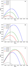 |
Fig. 1. Normalized growth rate, γ/ωpc vs. normalized wavenumber kλDc from Eq. (4) for the IIAI with parameters given by Table 1. Panels a, b, and c depict Series 1, 2, and 3, respectively, with the fiducial run shown by the gray curve. These theoretical expectations are compared with simulation results in Table 2. The vertical dashed lines refer to the simulated wavenumber (kλDc = 0.126). |
Key parameters of the runs under consideration.
2. Linear instability analysis and numerical simulations
We briefly recap the IIAI linear theory, which is used to validate our simulations. We consider a system comprising three species: core protons, beam protons, and background electrons. All species have Maxwellian VDFs. For collisionless unmagnetized plasma system the 1D-1V Vlasov equation reads as
 (1)
(1)
The electric potential φ can be calculated using Poisson’s equation
 (2)
(2)
where  is the number density; fs(v) is the VDF, with s = c for core protons, b for beam protons, and e for electrons; ms is the mass; and qs is the electric charge. The electrostatic potential and the electric field are related by E = −∂φ/∂x. In this study we initialize the core protons with a nondrifting Maxwellian, VD, c = 0, for all simulations, while the beam protons and electrons both have drifting Maxwellian distributions, expressed as
 (3)
(3)
where VD, s and  represent the drift and thermal velocities, with temperatures Ts given in energy units. The zero current condition demands nbVD, b − neVD, e = 0 when considering VD, c = 0 as the reference frame. The length, time, and velocity are normalized to the core Debye length
  , the core plasma frequency ωpc, and the core thermal velocity vth, c, respectively. We use a realistic mass ratio mi/me = 1836 and equal temperatures for the two proton populations Tb/Tc = 1. Within the framework of standard linear Landau theory, the dispersion relation for this system is derived by considering a linear perturbation around a homogeneous equilibrium.
Applying a standard plane-wave perturbation ansatz of the form ∼ei(kx − ωt) to the linearized system yields the following electrostatic dispersion relation (Gary & Omidi 1987; Afify et al. 2024):
 (4)
(4)
Here  , Z(ζj) is the plasma dispersion function (Fried & Conte 1961),
  , ω = ωr + iγ is the complex frequency, and k is the wavenumber.
The growth rate’s dependence on key system parameters is evident in Figs. 1 and 2, where we show results from IIAI linear theory and simulations, respectively, using the parameters listed in Table 1.
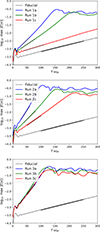 |
Fig. 2. Evolution of the electric field amplitude as a function of time for the simulation runs described in Table 1. In Table 2 we compare the growth rate measured here, illustrated with black lines, with linear theory. |
The simulation parameters in the table integrate our previous dilute-beam results (Afify et al. 2024) with new regimes motivated by in situ measurements of nonthermal ion populations (Verniero et al. 2020, 2022; Phan et al. 2022). The fiducial run maintains the core-beam configuration from Afify et al. (2024), but adopts an enhanced beam-core drift VD, b/vth, c = 5.7, consistent with PSP observations of the beam proton (Mozer et al. 2021a), where drifts of ∼180 km/s far exceeded the ion thermal speed of ∼27 km/s. Series 1–3 systematically probe critical parameter dependences: Series 1 varies Te/Tc to match the elevated electron-to-core temperature ratios (7 ≲ Te/Tc ≲ 10) measured during intervals of IAW activity (Píša et al. 2021; Mozer et al. 2022); Series 2 explores nb/nc values (0.1–0.3) spanning the transition from dilute beams in quiet solar wind to dense beams in magnetic reconnection regions (Phan et al. 2022); Series 3 probes VD, b/vth, c variations compatible with observations in Graham et al. (2021). This parameter space directly samples the conditions underlying the bursty IAWs reported in these studies (Mozer et al. 2021a; Píša et al. 2021; Graham et al. 2021; Mozer et al. 2022), enabling quantitative comparison between our predicted instability threshold and heating rates and observed nonthermal proton distributions.
In Fig. 1, panels a, b, and c, we depict Series 1, 2, and 3, respectively; the fiducial run is represented by the gray curve. We observe a strong enhancement in growth rate with increasing electron-to-core temperature ratio (panel a) and beam-to-core density ratio (panel b). In panel c we observe the same pattern relating increasing drift velocity and growth rate already described in Afify et al. (2024), Fig. 1: the growth rate first increases and then decreases with increasing core-to-beam drift.
These theoretical results (which are already well known) are confirmed by simulations. The simulations are run using a 1D1V Vlasov simulation framework (Afify et al. 2024, 2025). The simulation boxes have size Lx/λDc = 50, which selects the wavenumber kλDc = 0.126 if only one oscillation is present in the box. These values were selected to ensure that the simulations resolve a wavenumber close enough to that of maximum growth, according to linear theory analysis. The solver implements a finite-volume method to discretize the Vlasov equation on a two-dimensional coordinate-velocity phase-space grid. The evolution of the cell-averaged values of the distribution function, fs, is performed using a third-order Runge–Kutta scheme (Shu & Osher 1988). Periodic boundary conditions are applied along the x-axis, while zero-flux boundary conditions are imposed along the v-axis, ensuring the conservation of the total particle number within the domain for each species, except for the occasional resetting of negative undershoots in fsα to zero. The integration time step is chosen as Δt = 1/2500ωpc, as in Afify et al. (2024). Initial particle distribution functions are modeled as drifting Maxwellians according to Eq. (3). To excite the fundamental mode with parameters given by Table 1, a perturbation δV = 0.01sin((2π/Lx)x) is added to the beam drift velocity.
In Fig. 2 we show the evolution as a function of time of the maximum electric field value for Series 1, 2, and 3 runs in panels a, b, and c, respectively, where the fiducial simulation is presented by the gray curve. From these plots, we calculate the growth at the wavenumber k λDc = 0.126 selected by the simulation box length and we compare it, together with the real frequency, with results from linear theory in Table 2. We observe good agreement between the theoretical and simulated results.
3. Energy evolution
In this section we focus on energy exchange between fields and particles in our simulations. Multiplying Eq. (1) by  and then integrating over all coordinate (1D) and all velocity (1V) space yields
 (5)
(5)
The second term in Eq. (5) vanishes for periodic boundary conditions and for distributions that decay at infinity since it contributes only through boundary terms. We define the phase-space energy density for species s as  , which represents the energy density per unit length and per unit velocity in the 1D–1V Vlasov–Poisson system (Howes et al. 2017). The time evolution of the phase-space energy density, ∂ϵs(x, v, t)/∂t, can then be obtained from Eq. (5), yielding
 (6)
(6)
Therefore, Eq. (6) gives the instantaneous rate of energy transfer between the electric fields and the particle species, which is responsible for variation in particle energy. Integrating Eq. (6) over space, velocity, and time, one gets
 (7)
(7)
which is the nonlinear wave particle interaction term. The evolution of the electric field energy  and the microscopic particle energy
  is shown in Fig. 3 (panel a) for the fiducial simulation and in Fig. 4 for the other simulations in Table 1. The solid lines depict
 (8)
(8)
where s is the core, beam, electron, field, and total energy, and the subscript 0 labels the initial time. These values are obtained directly from the usual simulation diagnostics. The dashed lines similarly depict ℰs for the different particle populations as per Eq. (7).
We observe in Fig. 3, panel a, and in Fig. 4 that the solid and dashed lines superimpose for the particle populations, as they should since they represent different ways of calculating energy exchange for a particle species. The cyan curves track the total energy changes in the simulation (fields plus particles), and illustrate excellent energy conservation in our runs. We see in Fig. 3 that the main energy exchange is between the core and beam population: the beam loses energy, which is gained mostly by the core protons and, to a lesser extent, by the electrons. The energy gained by the electric field is small in comparison as the field acts primarily as a medium for energy transport between the particle species. In Fig. 3, panel b, we plot the energy variation of protons (core and beam) and of the electrons normalized to their respective initial energy, 𝒫s/𝒫s0. We see that the relative energy variation of the electron is minimal with respect to that of the core and beam protons: the electrons do not gain significant kinetic energy.
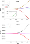 |
Fig. 3. Energy evolution in the fiducial run. Upper panel: Energy variation of the different particle populations (solid lines), the total energy, and the electric field energy (inset) calculated as Eq. (8). Also shown is the energy variation for the particle populations (dashed lines) calculated as Eq. (7). Lower panel: 𝒫s/𝒫s0 for the three particle populations and for the total energy. The horizontal solid magenta line at zero separates positive and negative values of 𝒫 and ℰ. |
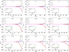 |
Fig. 4. Energy evolution for the three simulation series. The change in the particles, field, and total kinetic energy (solid lines, 𝒫), and the net energy exchange rate (dashed lines, ℰ), for Series 1 (first row), Series 2 (second row), and Series 3 (third row) runs in Table 1. Same as in Fig. 3, with the horizontal zero line indicating the separation between positive and negative values. |
In Fig. 4 we see that the amount of exchanged energy depends directly on the growth rate of the instability, as expected: higher growth rate is accompanied by a larger amount of exchanged energy. In the first line of Fig. 4 decreasing Te/Tc results in decreasing growth rate (Table 2); the 𝒫 components decrease in absolute value. In the second line of Fig. 4, decreasing nb/nc also results in lower growth rates (Table 2); again, the amount of energy exchanged between the population decreases. In the third line of Fig. 4, we see minimal difference in the amount of energy exchange as a function of increasing VD, b/vth, c, with respect to the larger variation observed in the first and the second row. The reason for this is clear from Fig. 2: the variation in growth rate between the three simulations is much smaller in Series 3 than in Series 1 and 2. The field energy evolution is depicted in the insets, and it exhibits the same pattern: weaker instabilities result in a smaller field energy increase and, consequently, weaker particle energization. Moreover, a decrease in Te/Tc, nb/nc, or VD, b/vth, c in all three parameter scans leads to a reduced electron energy gain relative to the beam’s energy loss. This suggests that when instability becomes less effective, electrons absorb a smaller percentage of the available energy, which results in a slight shift in the energy partition between the electrons and the beam, along with a decrease in the total energy exchanged.
4. Field particle correlation
Investigation of the evolution of VDFs and electromagnetic fields is constrained by the limitations of in situ observations, which typically rely on single-point measurements. Consequently, the nonlinear wave-particle interaction described by Eq. (6) presents a tailored methodology for examining the rate of change of phase-space energy density, as opposed to total energy, leveraging single-point time series measurements of electromagnetic fields and VDFs. The field-particle correlation (FPC) technique quantifies energy transfer by correlating the electric field (which alone performs work) with the velocity derivative of the VDF. This single-point measurement approach reveals the velocity-space structure of the field-particle energy exchange, which can be tied to specific energization and instability processes. The FPC approach is fundamentally applicable to single-point spacecraft measurements, providing a powerful tool for analyzing particle energization mechanisms in weakly collisional heliospheric plasmas.
To differentiate between oscillatory energy exchange associated with wave motion and secular energy exchange resulting from net energy transfer between particles and fields, the FPC method performs a time average over an interval τ = NΔt exceeding the linear wave period (i.e.,  for the dominant oscillations). This isolates the secular component of the energy transfer, while the oscillatory component, representing reversible energy exchange, is eliminated. The field-particle correlation at time ti and position x0, computed over an interval τ = N Δt, is given by (Klein et al. 2017)
 (9)
(9)
where the term that enters the summation is the right-hand side of Eq. (6) evaluated at a single point in space, x = x0. By integrating over all spatial positions, we can compare FPC to the variation in species energy in Eq. (7) at a given time t′. By analyzing single-point measurements at position x = x0 we can obtain a map of FPC for each particle species, s, as a function of velocity and time, from which we can directly see at which velocities energy is exchanged by that species with the electric field, if the exchange is secular or the result of oscillations, and if the particle species gains (positive sign) or loses (negative sign) energy.
In the following subsections, we examine FPC as a function of velocity and integrated over velocity, ∫dvFPC(x0, v, ti, τ). Our goal is to look for phase-space signatures at a specific spatial location for each simulation run listed in Table 1. Moreover, we show the transfer of secular energy in the species phase space by averaging over a time interval larger than the linear wave period.
4.1. Fiducial run
In Fig. 5 we plot ∫dvFPC, which quantifies the interaction between the electric field E and the three plasma populations over correlation intervals τωpc ∈ [0, 100]. The quantity is depicted in normalized units that follow from the code normalization described in Sect. 2. With the real frequencies of our instabilities in the range ωr/ωpc ∼ 0.2 − 0.4, our minimum correlation interval is in the range ωpcτmin ∼ 15 − 30. The field-particle correlation technique is evaluated at x/λDc = 0. In the fiducial run, a pronounced oscillatory energy exchange occurs at short correlation times (τ), but no single τ value entirely removes the oscillatory energy transfer for electrons. However, evidence of secular energy transfer is observed for both the beam (energy decrease) and the core (energy increase) protons. The FPC map in Fig. 6, panel a and b, reveals that both core and beam exchange energy with the fields in an oscillatory pattern over a large range of velocities: at fixed velocity, positive and negative signatures follow each other in time. Secular energy exchange is observed at the resonant velocity (dashed vertical line, refer to Table 2 for resonant velocities in all runs): the beam loses energy (negative blue signature, positive ∂fpj/∂v in Eq. (9)), which drives the instability. Instead, the core gains energy (positive red signature, negative positive ∂fpj/∂v in Eq. (9)). We do not observe secular energy exchange for the electrons, panel c, which just exhibit an oscillating pattern. In panel d we integrate energy exchange for the different particle populations in velocity at the same spatial position, x/λDc = 0, and using τωpc = 100: we observe an oscillatory behavior for beam protons and electrons, but not for the core. We observe in the subsequent analysis (Figs. 8, 10, 12, and 13) that oscillations are visible in the energy evolution of electrons and beam when the growth rate is low.
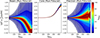 |
Fig. 5. ∫dv FPC for a range of correlation intervals of RUN Fiducial at x/λDc = 0. |
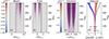 |
Fig. 6. Velocity-dependent FPC for RUN Fiducial at x/λDc = 0 for beam, core, and electrons (panels a, b, and c, respectively) for a correlation interval of τωpc = 30. Panel d: ∫dv FPC The correlation interval τωpc is set to 100. The vertical dashed lines indicate the resonant velocity, which is 3.333 vth, c. |
4.2. Series 1: Varying electron temperature
Figures 7 and 8 refer to Series 1 simulations, where we decrease the electron-to-core temperature ratio. This quantity (Te/Tc) significantly alters the IIAI growth rate, and hence the energy exchange dynamics. This dependence arises from the shift of the ion-acoustic phase speed, and therefore of the resonance velocity, relative to the proton velocity distributions. While the pattern of energy exchange is consistent with the fiducial run (the beam secularly loses energy, the core gains it), the amount of exchanged energy decreases significantly with decreasing Te/Tc (rows 1–3), and hence decreasing growth rate, as the resonance velocity moves toward regions of weaker positive velocity-space gradient in the beam distribution. ∫dvFPC (Fig. 7) shows that oscillatory energy exchange diminishes with longer τ, shifting toward secular transfer; with longer correlation intervals, oscillations in energy transfer are averaged out. The FPC plots (Fig. 8) are consistent with those for the fiducial run, confirming that proton dynamics remain tied to ion-acoustic resonances occurring near the resonance velocity. When the IIAI growth rate is higher for larger Te/Tc, the resonance velocity lies in a region where the total proton distribution, fp = fc + fb, exhibits a strong positive velocity-space gradient, resulting in efficient secular energy transfer. In this case, oscillatory energy exchange is not visible in the v-integrated energy exchange plots in Fig. 8, panel d. It becomes visible with decreasing growth rate, as the resonance velocity shifts away from this region and secular exchange weakens.
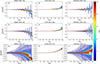 |
Fig. 7. ∫dvFPC for a range of correlation intervals for Series 1 runs at x/λDc = 0. Runs 1, 2, and 3 are shown from top to bottom. |
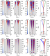 |
Fig. 8. Velocity-dependent FPC for Series 1 runs at x/λDc = 0. The correlation interval τωpc is set to 100 for protons and 10 for electrons, except in Case 1c, where it is set to 10 for both protons and electrons. The vertical dashed lines indicate the resonant velocities, which are 3.377, 3.333, and 3.284 (from top to bottom). |
4.3. Series 2: Varying proton beam density
Figures 9 and 10 refer to Series 2 simulations, where we reduce the beam-to-core density ratio. We observe reduced energy exchange with decreasing beam density, and hence a reduced growth rate as fewer beam particles are available to resonate with the ion-acoustic wave at the resonance velocity. As expected, secular energy exchange for both beam and core populations occurs at the resonant velocity. In all three cases explored here, the IIAI growth rate remains sufficiently high that the secular energy exchange dominates and masks the oscillatory energy exchange behavior in panels d of Fig. 10.
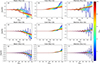 |
Fig. 9. Net energy transfer rate over a range of correlation intervals for Series 2 x/λDc = 0, arranged in the same format as in Fig. 7. |
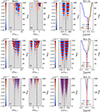 |
Fig. 10. Velocity-dependent FPC for Series 2 runs at x/λDc = 0. The correlation interval τωpc is set to 100. The vertical dashed lines indicate the resonant velocities, which are 3.295, 3.481, and 3.583 (from top to bottom). |
4.4. Run 3: Varying drift speed
Figures 11 and 12 refer to Series 3, where we reduce the beam drift speed. The observed behavior is consistent with that shown in Figs. 9 and 11, and in Figs. 10 and 12. In this parameter scan, changes in the drift speed primarily modify the relative position of the resonance velocity with respect to the beam distribution, leading to variations in growth rate and energy exchange that follow the same resonance-controlled trends observed in the previous series.
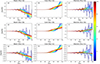 |
Fig. 11. ∫dvFPC for a range of correlation intervals of Series 3 runs at x/λDc = 0, arranged in the same format as in Fig. 7. |
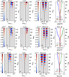 |
Fig. 12. Velocity-dependent FPC for Series 3 runs at x/λDc = 0. The correlation interval τωpc is set to 100. The vertical dashed lines indicate the resonant velocities, which are 3.408, 3.114, and 2.909 (from top to bottom). |
4.5. Energy transfer as functions of simulation position
Until now, we have evaluated FPC at a fixed position, x/λDc = 0. Now we want to examine how FPC traces change in different areas of the domain. For this analysis, we use Run 2b, where the secular energy exchange between species is high enough to mask oscillatory energy exchange. Similar considerations hold for the other simulations. In Fig. 13 we depict the velocity-integrated FPC as a function of time at position x0/λDc = 0, 12.5, 25, 37.5, respectively. We see that the core proton signature does not change significantly with position. The beam signatures stay negative after instability onset, with values at a fixed time changing slightly as a function of the sampling point position. The electron signature is the one that changes more significantly after instability onset, from positive at position x0/λDc = 0, 37.5 to close to zero at x0/λDc = 12.5, 25. We understand the reason for this behavior from Fig. 14, where we plot the phase space for beam, core, and electrons at time ωpct = 130, marked as a horizontal line in Fig. 13. For completeness, we plot in panel d the electric field as a function of space. The location of the sampling points in Fig. 13 are marked as vertical lines in Fig. 14. We see that the core phase space changes minimally with x in Fig. 14, panel b; as already highlighted in Afify et al. (2025), among others, the core is minimally affected by IIAI at least in these parameter regimes. In panel a, we see that the beam protons develop into an ion hole, which is obviously spatially dependent. This is the reason for the slight variation in the beam signature with space in Fig. 13. The electrons react to the ion hole and to the corresponding electric field by exhibiting a slight increase in phase-space density in correspondence with the electric field zero at x/λDc ∼ 7.8. This spatial variation is reflected in Fig. 13. The dependence of FPC signatures with position, and their relation with the nodes and antinodes of the fields in the case of instabilities has already been highlighted in Klein (2017).
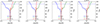 |
Fig. 13. Velocity integrated FPC as a function of time for run 2B, evaluated at positions x/λdc = 0, 12.5, 25, 37.5 (from left to right). The horizontal line marks ωpct = 130. |
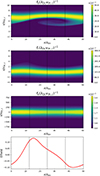 |
Fig. 14. Phase space for beam, core, electrons (panels a to c) and electric field (panel d) for the 2b run at ωpct = 130. The vertical lines mark x/λDc = 0, 12.5, 25, 37.5. |
5. Summary and discussion
For this paper we applied FPC to fully kinetic simulations of the IIAI, often observed in the young solar wind. Our aim was to use fully kinetic simulations to identify characteristic IIAI FPC signatures and to make future identification of IIAI in observations more efficient. For this reason, our simulations are in parameter regimes compatible with observed solar wind properties. First, in Figs. 3 and 4, we examine energy transfer in the simulations, using both diagnostics readily available in simulations (Eq. (8)) and the nonlinear wave particle interaction term which constitutes the base of FPC (Eq. (7)). Both approaches deliver the same results since they are different ways of calculating the same quantity. This analysis confirms that the proton beam is the primary instability driver, i.e., the particle population whose energy powers the instability (see Figs. 3 and 4). The majority of the energy lost by the beam population is gained by the core population, with energy transfer increasing with the growth rate of the instability (Fig. 4). The energy gained by the electron population is non-negligible in absolute terms (Fig. 3, upper panel), but small with respect to their initial energy (Fig. 3, lower panel).
We examined the effects of using different FPC correlation intervals for our analysis (Figs. 5, 7, 9, 11). We find that τ = 100ωpc, which corresponds to τ/T ∼ 8, with T = 2π/ω, is a value capable of highlighting secular versus oscillatory energy transfer. We then looked for characteristic FPC signatures for the different particle populations (Figs. 6, 8, 10, 12). Integrating FPC in velocity space (fourth panel in each row in Figs. 6, 8, 10, 12), we observe that the oscillations in the proton beam and electron signatures and associated with oscillatory energy exchange patterns are dominated by secular exchange when the IIAI growth rate is high. Examining FPC signatures as a function of time in velocity space (first three panels in Figs. 6, 8, 10, 12), we observe traces of secular and resonant energy transfer in correspondence of the IA resonance velocity for both the proton beam (first panel) and core (second panel): the beam loses energy, while the core gains it. Instead, the electrons (third panel) exhibit only an oscillatory energy exchange pattern between the fields and the particles. Changing the key parameters that determine the growth rate (Te/Tc, nb/nc, and VD, b/vth, c) we observe a strong positive correlation between the growth rate and the exchanged energy. The ratio of energy exchange between different particle components appears consistent across growth rates. Investigating the impact of probe location in simulations gives quite interesting results (Figs. 13 and 14). We observe that energy transfer for the proton core population is not affected by probe location since the core proton population is minimally affected by the formation of ion holes generated by the IIAI. Proton beam and electron results, instead, show position dependence, since both the proton beam and electron velocity distribution are affected by ion holes; ion holes are constituted of beam protons, but modify the electron velocity distribution as well through electric field modulation (Fig. 14).
Although the present analysis is not designed to model spacecraft sampling effects such as Doppler shifting and sampling frequencies, the results are nonetheless relevant for the interpretation of single-point measurements. A detailed quantification of these effects applied specifically to PSP and Solar Orbiter measurements will be addressed in future studies. The FPC technique is intrinsically a single-spacecraft diagnostic, depending only on local time series of the electric field and particle velocity distribution functions. The velocity-space signatures of IIAI identified here therefore provide a physically grounded reference for what such instabilities would produce in idealized single-point measurements.
A natural future outlook for this investigation is to look for the IIAI FPC signatures identified here in observations of the young solar wind. This task will be left for future missions supporting higher instrumental cadence, since PSP’s SPANi fastest possible cadence is 0.87 s (Livi et al. 2022). As remarked in Malaspina et al. (2024), this is too slow to capture proton signatures of ongoing IIAI dynamics if the timescale of the IIAI (inverse of the growth rate) is on the order of tens of milliseconds, as obtained in this and previous work (Afify et al. 2024) in parameter ranges compatible with observations. In addition, evolution times on the order of a few percent of the ion gyrofrequency are too fast for direct PSP sampling if the gyrofrequency is calculated with magnetic field values on the order of B = 200 nT, as reported in correspondence with IIAI observations in Mozer et al. (2023b), Table 1.
Future work will examine more realistic simulation scenarios that take into account both the anisotropies in the different particle populations frequently observed in the solar wind and the possible role of larger-scale processes (e.g., magnetic reconnection) in the production of ion beams that result in IIAI.
Acknowledgments
M. S. Afify thanks the Alexander-von-Humboldt Foundation, 53173 Bonn, Germany (Ref 3.4-1229224-EGY-HFST-P) for the research fellowship and its financial support. M.E.I. acknowledges support from the Deutsche Forschungsgemeinschaft (DFG, German Research Foundation) within the Collaborative Research Center SFB1491 and project 497938371. We thank Jürgen Dreher for the useful discussions on the optimization of the Vlasov code used in this study.
References
- Afify, M. S., Dreher, J., Schoeffler, K., Micera, A., & Innocenti, M. E. 2024, ApJ, 971, 93 [Google Scholar]
- Afify, M. S., Dreher, J., O’Neill, S., & Innocenti, M. E. 2025, A&A, 702, A277 [NASA ADS] [CrossRef] [EDP Sciences] [Google Scholar]
- Afshari, A., Howes, G., Kletzing, C., Hartley, D., & Boardsen, S. 2021, J. Geophys. Res.: Space Phys., 126, e2021JA029578 [Google Scholar]
- Afshari, A., Howes, G., Shuster, J., et al. 2024, Nat. Commun., 15, 7870 [Google Scholar]
- Baumjohann, W., & Treumann, R. A. 2012, Basic Space Plasma Physics (World Scientific) [Google Scholar]
- Boldú, J. J., Graham, D., Morooka, M., et al. 2024, Geophys. Res. Lett., 51, e2024GL109956 [Google Scholar]
- Brown, C. R., Juno, J., Howes, G. G., Haggerty, C. C., & Constantinou, S. 2023, J. Plasma Phys., 89, 905890308 [Google Scholar]
- Cattell, C., Breneman, A., Dombeck, J., et al. 2022, ApJ, 924, L33 [NASA ADS] [CrossRef] [Google Scholar]
- Chen, C., Klein, K., & Howes, G. G. 2019, Nat. Commun., 10, 740 [CrossRef] [Google Scholar]
- Dai, L., Wang, C., & Lavraud, B. 2021, ApJ, 919, 15 [Google Scholar]
- Fox, N. J., Velli, M. C., Bale, S. D., et al. 2016, Space Sci. Rev., 204, 7 [Google Scholar]
- Fried, B. D., & Conte, S. D. 1961, The Plasma Dispersion Function: The Hilbert Transform of the Gaussian (Elsevier Inc.) [Google Scholar]
- Gary, S. P. 1993, Theory of Space Plasma Microinstabilities (New York: Cambridge Univ. Press) [Google Scholar]
- Gary, S. P., & Omidi, N. 1987, J. Plasma Phys., 37, 45 [CrossRef] [Google Scholar]
- González, C., Innocenti, M. E., & Tenerani, A. 2023, J. Plasma Phys., 89, 905890208 [Google Scholar]
- Goodrich, K. A., Ergun, R., Schwartz, S. J., et al. 2019, J. Geophys. Res. Space Phys., 124, 1855 [Google Scholar]
- Graham, D. B., Khotyaintsev, Y. V., Sorriso-Valvo, L., et al. 2021, A&A, 656, A23 [NASA ADS] [CrossRef] [EDP Sciences] [Google Scholar]
- Graham, D., Cozzani, G., Khotyaintsev, Y. V., et al. 2025a, Space Sci. Rev., 221, 20 [Google Scholar]
- Graham, D. B., Khotyaintsev, Y. V., & Lalti, A. 2025b, arXiv e-prints [arXiv:2502.07953] [Google Scholar]
- Gurnett, D. A. 1991, in Waves and Instabilities, eds. R. Schwenn, & E. Marsch (Berlin, Heidelberg: Springer-Verlag), 135 [Google Scholar]
- Gurnett, D. A., & Anderson, R. R. 1977, J. Geophys. Res., 82, 632 [NASA ADS] [CrossRef] [Google Scholar]
- Hollweg, J. V. 1975, Rev. Geophys., 13, 263 [Google Scholar]
- Howes, G. G. 2024, J. Plasma Phys., 90, 905900504 [Google Scholar]
- Howes, G. G., Klein, K. G., & Li, T. C. 2017, J. Plasma Phys., 83, 705830102 [Google Scholar]
- Howes, G. G., Felix, A., Brown, C. R., et al. 2025, Phys. Plasmas, 32, 6 [Google Scholar]
- Huang, R., Howes, G. G., & McCubbin, A. J. 2024, J. Plasma Phys., 90, 535900401 [Google Scholar]
- Juno, J., Brown, C. R., Howes, G. G., et al. 2023, ApJ, 944, 15 [Google Scholar]
- Klein, K. G. 2017, Phys. Plasmas, 24, 5 [Google Scholar]
- Klein, K. G., & Howes, G. G. 2016, ApJ, 826, L30 [Google Scholar]
- Klein, K. G., Howes, G. G., & TenBarge, J. M. 2017, J. Plasma Phys., 83, 535830401 [Google Scholar]
- Klein, K. G., Howes, G. G., TenBarge, J. M., & Valentini, F. 2020, J. Plasma Phys., 86, 905860402 [Google Scholar]
- Kurth, W., Gurnett, D., & Scarf, F. 1979, J. Geophys. Res., 82, 632 [Google Scholar]
- Li, D., Liu, Z., & Loureiro, N. F. 2025, arXiv e-prints [arXiv:2505.08983] [Google Scholar]
- Liu, Z., White, R., Francisquez, M., Milanese, L. M., & Loureiro, N. F. 2024, J. Plasma Phys., 90, 965900101 [Google Scholar]
- Livi, R., Larson, D. E., Kasper, J. C., et al. 2022, ApJ, 938, 138 [NASA ADS] [CrossRef] [Google Scholar]
- Malaspina, D. M., Ergun, R. E., Cairns, I. H., et al. 2024, ApJ, 969, 60 [Google Scholar]
- Mangeney, A., Salem, C., Lacombe, C., et al. 1999, Ann. Geophys., 17, 307 [NASA ADS] [CrossRef] [Google Scholar]
- Marsch, E. 1991, in Physics of the Inner Heliosphere II: Particles, Waves and Turbulence (Springer), 45 [Google Scholar]
- Montag, P., & Howes, G. G. 2022, Phys. Plasmas, 29, 032901 [Google Scholar]
- Montag, P., Howes, G., McGinnis, D., et al. 2025, ApJ, 980, L23 [Google Scholar]
- Mozer, F. S., Bonnell, J. W., Bowen, T. A., Schumm, G., & Vasko, I. Y. 2020, ApJ, 901, 107 [NASA ADS] [CrossRef] [Google Scholar]
- Mozer, F. S., Vasko, I. Y., & Verniero, J. L. 2021a, ApJ, 919, L2 [NASA ADS] [CrossRef] [Google Scholar]
- Mozer, F. S., Bonnell, J. W., Hanson, E. L. M., Gasque, L. C., & Vasko, I. Y. 2021b, ApJ, 911, 89 [CrossRef] [Google Scholar]
- Mozer, F. S., Bale, S. D., Cattell, C. A., et al. 2022, ApJ, 927, L15 [NASA ADS] [CrossRef] [Google Scholar]
- Mozer, F., Bale, S., Kellogg, P., et al. 2023a, Phys. Plasmas, 062111, 30 [Google Scholar]
- Mozer, F. S., Agapitov, O. V., Kasper, J. C., et al. 2023b, A&A, 673, L3 [NASA ADS] [CrossRef] [EDP Sciences] [Google Scholar]
- Müller, D., Cyr, O. S., Zouganelis, I., et al. 2020, A&A, 642, A1 [NASA ADS] [CrossRef] [EDP Sciences] [Google Scholar]
- Nair, R., Halekas, J. S., Cattell, C., et al. 2025, ApJ, 984, 14 [Google Scholar]
- Perrone, D., Valentini, F., & Veltri, P. 2011, ApJ, 741, 43 [Google Scholar]
- Phan, T. D., Verniero, J. L., Larson, D., et al. 2022, Geophys. Res. Lett., 49, e2021GL096986 [Google Scholar]
- Píša, D., Soucek, J., Santolík, O., et al. 2021, A&A, 656, A14 [NASA ADS] [CrossRef] [EDP Sciences] [Google Scholar]
- Shu, C.-W., & Osher, S. 1988, J. Comput. Phys., 77, 439 [NASA ADS] [CrossRef] [Google Scholar]
- Stix, T. 1992, Waves in Plasmas (New York: American Institute of Physics) [Google Scholar]
- Tenerani, A., Sioulas, N., Matteini, L., et al. 2021, ApJ, 919, L31 [NASA ADS] [CrossRef] [Google Scholar]
- Valentini, F., Perrone, D., & Veltri, P. 2011, ApJ, 739, 54 [NASA ADS] [CrossRef] [Google Scholar]
- Valentini, F., Vecchio, A., Donato, S., et al. 2014, ApJ, 788, L16 [NASA ADS] [CrossRef] [Google Scholar]
- Verniero, J. L., Larson, D., Bowen, T. A., et al. 2020, ApJS, 248, 5 [Google Scholar]
- Verniero, J., Howes, G., Stewart, D., & Klein, K. 2021, J. Geophys. Res.: Space Phys., 126, e2020JA028361 [Google Scholar]
- Verniero, J. L., Chandran, B. D. G., Larson, D. E., et al. 2022, ApJ, 924, 112 [NASA ADS] [CrossRef] [Google Scholar]
- Wilson, L., III, Cattell, C., Kellogg, P., et al. 2007, Phys. Rev. Lett., 99, 041101 [Google Scholar]
All Tables
All Figures
|
Fig. 1. Normalized growth rate, γ/ωpc vs. normalized wavenumber kλDc from Eq. (4) for the IIAI with parameters given by Table 1. Panels a, b, and c depict Series 1, 2, and 3, respectively, with the fiducial run shown by the gray curve. These theoretical expectations are compared with simulation results in Table 2. The vertical dashed lines refer to the simulated wavenumber (kλDc = 0.126). |
| In the text | |
|
Fig. 2. Evolution of the electric field amplitude as a function of time for the simulation runs described in Table 1. In Table 2 we compare the growth rate measured here, illustrated with black lines, with linear theory. |
| In the text | |
|
Fig. 3. Energy evolution in the fiducial run. Upper panel: Energy variation of the different particle populations (solid lines), the total energy, and the electric field energy (inset) calculated as Eq. (8). Also shown is the energy variation for the particle populations (dashed lines) calculated as Eq. (7). Lower panel: 𝒫s/𝒫s0 for the three particle populations and for the total energy. The horizontal solid magenta line at zero separates positive and negative values of 𝒫 and ℰ. |
| In the text | |
|
Fig. 4. Energy evolution for the three simulation series. The change in the particles, field, and total kinetic energy (solid lines, 𝒫), and the net energy exchange rate (dashed lines, ℰ), for Series 1 (first row), Series 2 (second row), and Series 3 (third row) runs in Table 1. Same as in Fig. 3, with the horizontal zero line indicating the separation between positive and negative values. |
| In the text | |
|
Fig. 5. ∫dv FPC for a range of correlation intervals of RUN Fiducial at x/λDc = 0. |
| In the text | |
|
Fig. 6. Velocity-dependent FPC for RUN Fiducial at x/λDc = 0 for beam, core, and electrons (panels a, b, and c, respectively) for a correlation interval of τωpc = 30. Panel d: ∫dv FPC The correlation interval τωpc is set to 100. The vertical dashed lines indicate the resonant velocity, which is 3.333 vth, c. |
| In the text | |
|
Fig. 7. ∫dvFPC for a range of correlation intervals for Series 1 runs at x/λDc = 0. Runs 1, 2, and 3 are shown from top to bottom. |
| In the text | |
|
Fig. 8. Velocity-dependent FPC for Series 1 runs at x/λDc = 0. The correlation interval τωpc is set to 100 for protons and 10 for electrons, except in Case 1c, where it is set to 10 for both protons and electrons. The vertical dashed lines indicate the resonant velocities, which are 3.377, 3.333, and 3.284 (from top to bottom). |
| In the text | |
|
Fig. 9. Net energy transfer rate over a range of correlation intervals for Series 2 x/λDc = 0, arranged in the same format as in Fig. 7. |
| In the text | |
|
Fig. 10. Velocity-dependent FPC for Series 2 runs at x/λDc = 0. The correlation interval τωpc is set to 100. The vertical dashed lines indicate the resonant velocities, which are 3.295, 3.481, and 3.583 (from top to bottom). |
| In the text | |
|
Fig. 11. ∫dvFPC for a range of correlation intervals of Series 3 runs at x/λDc = 0, arranged in the same format as in Fig. 7. |
| In the text | |
|
Fig. 12. Velocity-dependent FPC for Series 3 runs at x/λDc = 0. The correlation interval τωpc is set to 100. The vertical dashed lines indicate the resonant velocities, which are 3.408, 3.114, and 2.909 (from top to bottom). |
| In the text | |
|
Fig. 13. Velocity integrated FPC as a function of time for run 2B, evaluated at positions x/λdc = 0, 12.5, 25, 37.5 (from left to right). The horizontal line marks ωpct = 130. |
| In the text | |
|
Fig. 14. Phase space for beam, core, electrons (panels a to c) and electric field (panel d) for the 2b run at ωpct = 130. The vertical lines mark x/λDc = 0, 12.5, 25, 37.5. |
| In the text | |
Current usage metrics show cumulative count of Article Views (full-text article views including HTML views, PDF and ePub downloads, according to the available data) and Abstracts Views on Vision4Press platform.
Data correspond to usage on the plateform after 2015. The current usage metrics is available 48-96 hours after online publication and is updated daily on week days.
Initial download of the metrics may take a while.