| Issue |
A&A
Volume 707, March 2026
|
|
|---|---|---|
| Article Number | A6 | |
| Number of page(s) | 20 | |
| Section | Stellar structure and evolution | |
| DOI | https://doi.org/10.1051/0004-6361/202558123 | |
| Published online | 25 February 2026 | |
A 500 pc volume-limited sample of hot subluminous stars
II. Atmospheric parameters, mass distribution, and kinematics
1
Institute for Physics and Astronomy, University of Potsdam Karl-Liebknecht-Str. 24/25 14476 Potsdam, Germany
2
Department of Physics, University of Warwick Gibet Hill Road Coventry CV4 7AL, UK
3
Dr. Remeis-Sternwarte and ECAP, Astronomical Institute, University of Erlangen-Nürnberg Sternwartstr. 7 D-96049 Bamberg, Germany
4
Instituto de Física y Astronomía, Universidad de Valparaíso Gran Bretaña 1111 Playa Ancha Valparaíso 2360102, Chile
5
European Southern Observatory Alonso de Cordova 3107 Santiago, Chile
6
Institute of Astronomy, KU Leuven Celestijnenlaan 200D B-3001 Leuven, Belgium
7
Thüringer Landessternwarte Tautenburg Sternwarte 5 D-07778 Tautenburg, Germany
8
Landessternwarte Heidelberg, Zentrum fur Astronomie, Ruprecht-Karls-Universitat Konigstuhl 12 69117 Heidelberg, Germany
9
Universitat Politècnica de Catalunya, Departament de Física c/ Esteve Terrades 5 08860 Castelldefels, Spain
10
Department of Astrophysics/IMAPP, Radboud University P O Box 9010 NL-6500 GL Nijmegen, The Netherlands
11
Max Planck Institut für Astrophysik Karl-Schwarzschild-Straße 1 85748 Garching bei München, Germany
12
Recogito AS Storgaten 72 N-8200 Fauske, Norway
13
Nordic Optical Telescope Rambla José Ana Fernández Pérez 7 ES-38711 Breña Baja, Spain
14
Department of Physics and Astronomy, Aarhus University Munkegade 120 DK-8000 Aarhus C, Denmark
15
Isaac Newton Group of Telescopes Apartado de Correos 368 E-38700 Santa Cruz de La Palma, Spain
16
Department of Physics and Astronomy, University of Sheffield Sheffield S3 7RH, UK
17
Nicolaus Copernicus Astronomical Centre ul. Rabiańska 8 87-100 Toruń, Poland
18
School of Science, University of New South Wales, Australian Defence Force Academy Canberra ACT 2600, Australia
19
Leuven Gravity Institute, KU Leuven Celestijnenlaan 200D box 2415 3001 Leuven, Belgium
20
Institut für Astrophysik und Geophysik, Georg-August-Universität Göttingen Friedrich-Hund-Platz 1 37077 Göttingen, Germany
★ Corresponding author: This email address is being protected from spambots. You need JavaScript enabled to view it.
Received:
14
November
2025
Accepted:
4
January
2026
Abstract
We present a quantitative spectroscopic and kinematic analysis of a volume-complete sample of hot subluminous stars within 500 pc of the Sun, assembled using accurate parallax measurements from the Gaia space mission Data Release 3 (DR3). In total, 3226 spectra of 253 hot subdwarf stars were analysed to derive atmospheric parameters (Teff, log g, and helium abundance) and radial velocities. Spectral energy distributions (SEDs) with Gaia parallaxes were used to measure stellar radii, luminosities, and masses. The derived atmospheric parameters reveal a consistent alignment between sdB and sdO stars in the Kiel diagram when compared to theoretical evolutionary models. Notably, we find a substantial population (about 10%) of hot subdwarfs located below the 0.45 M⊙ zero-age extreme horizontal branch (EHB) in both the Kiel and Hertzsprung-Russell diagrams (HRDs), which likely originate from intermediate-mass progenitors (1.8–8 M⊙). The overall mass distribution peaks at 0.48−0.10+0.14 M⊙, while hot subdwarfs below the EHB peak at 0.43−0.09+0.11 M⊙, supporting a scenario of non- or semi-degenerate helium ignition for these objects characteristic of intermediate-mass stars. Interpolation of EHB and post-EHB tracks yields theoretical mass distributions consistent with our estimates based on SED and parallax. By assuming a mass range between 0.40 and 0.50 M⊙ during the interpolation, we further find that the post-EHB birthrate in our sample is 2–3 times higher than the EHB birthrate, which may suggest overestimated EHB lifetimes in theoretical tracks or contamination from other formation and evolutionary channels. Our kinematic analysis shows that 86 ± 2% of the stars belong to the Galactic thin disk, with 13 ± 1% and 1 ± 1% associated with the thick disk and halo, respectively. The below-EHB population is exclusively found in the thin disk, the only Galactic population young enough to harbour intermediate-mass stars. The below-EHB population seems to be absent in other large samples, which generally include more thick disk and halo members. These findings suggest that non-degenerate formation channels may play a more prominent role in the Galactic disk than previously thought.
Key words: catalogs / binaries: general / stars: evolution / Hertzsprung-Russell and C-M diagrams / stars: statistics / subdwarfs
© The Authors 2026
 Open Access article, published by EDP Sciences, under the terms of the Creative Commons Attribution License (https://creativecommons.org/licenses/by/4.0), which permits unrestricted use, distribution, and reproduction in any medium, provided the original work is properly cited.
This article is published in open access under the Subscribe to Open model. This email address is being protected from spambots. You need JavaScript enabled to view it. to support open access publication.
1. Introduction
Hot subdwarf stars are compact, typically helium-burning stars that have lost nearly all of their hydrogen envelopes. As a result, they are found on or near the extreme end of the horizontal branch (EHB; Greenstein & Sargent 1974; Newell 1973; Heber et al. 1984) in the Hertzsprung–Russell diagram (HRD), marking a transitional evolutionary phase between the first red giant branch (RGB) and the white dwarf cooling sequence. B-type hot subdwarfs (sdBs) are thought to be powered by core helium fusion and generally exhibit helium-poor atmospheres, with effective temperatures between 20 000 and 40 000 K and surface gravities ranging from ∼4.75 to 6.75 dex. In contrast, the more evolved O-type subdwarfs (sdOs), which are assumed to be sustained by helium shell burning, show a broader range of helium abundances and temperatures extending from 40 000 K up to ∼80 000 K, along with slightly wider ranges of surface gravities and radii (for comprehensive reviews, see Heber 2009, 2016, 2026). Higher luminosity H-rich post-asymptotic giant branch (post-AGB) stars and central stars of planetary nebulae with surface gravities between roughly 4.5 and 5.5 dex are often spectroscopically classified as sdO as well, or as O(H) (Reindl et al. 2016, 2024).
The formation of hot subdwarf stars remains an open question. Since most sdBs have masses of about half a solar mass (Dorman et al. 1993; Fontaine et al. 2012; Schaffenroth et al. 2022), close to the core-helium-flash mass, they are thought to descend from low-mass stars (0.7–1.8 M⊙) that have lost almost all of their H envelopes while igniting helium under electron-degenerate conditions near the tip of the RGB. Such stars are typically referred to as canonical hot subdwarfs. However, intermediate-mass (1.8–8 M⊙) progenitors can ignite helium under semi- or non-degenerate conditions (without a flash) in the subgiant or Hertzsprung gap phases. The resulting He-burning core masses can be as low as ∼0.33 M⊙ depending on the progenitor masses (Han et al. 2002; Hu et al. 2008; Prada Moroni & Straniero 2009; Götberg et al. 2018; Arancibia-Rojas et al. 2024).
Although the predicted properties of He-burning cores closely resemble the observational properties of sdO/Bs, it is difficult to explain their extremely thin or completely missing hydrogen envelopes. The prevailing view is that binary interaction plays a crucial role in hot subdwarf formation (Pelisoli et al. 2020), following the evolutionary channels detailed in Han et al. (2002, 2003). Binary population synthesis (BPS) studies suggest three main formation channels for hot subdwarfs. Stable Roche lobe overflow (RLOF) from a RGB star to a main-sequence (MS) companion of FGK-type can lead to hot subdwarfs in binaries with long orbital periods (500–1500 d; Vos et al. 2020). For low-mass companions, the mass transfer becomes unstable and leads to common envelope (CE) evolution, yielding hot subdwarfs with M-type MS, brown dwarf, or white dwarf companions on short-period orbits (hours to days; Schaffenroth et al. 2022). Finally, helium-rich sdO (He-sdO) stars are suggested to form through the late ignition of He-burning triggered by mergers involving He-core white dwarfs (Webbink 1984). Related stars suggested to form through white dwarf mergers include the cooler and extreme helium (EHe) stars (Jeffery & Zhang 2020), as well as the hotter O(He) stars (Reindl et al. 2014). Single star evolution channels remain under discussion, such as internal mixing mechanisms in the hot flasher scenario (see e.g. Sweigart 1997; Castellani & Castellani 1993; Lanz et al. 2004; Miller Bertolami et al. 2008; Battich et al. 2018).
Current spectroscopic samples of hot subdwarfs, such as those based on the Sloan Digital Sky Survey (SDSS; Geier et al. 2017; Kepler et al. 2019; Geier et al. 2024), the Large Sky Area Multi-Object Fiber Spectroscopic Telescope (LAMOST; Lei et al. 2018, 2019, 2020, 2023a; Luo et al. 2019, 2021), or literature compilations (Geier 2020; Culpan et al. 2022) are affected by strong selection effects. With the advent of the Gaia survey, all-sky volume-complete samples can be characterised in detail by combining spectroscopic and kinematic properties of the local stellar population. In Dawson et al. (2024) (hereafter Paper I), we took the first step towards this goal by compiling a spectroscopically complete, volume-limited hot subdwarf sample to 500 pc, and presented classifications and a detailed discussion of space densities and spatial distributions. Our 500 pc sample, constructed using precise parallax measurements from Gaia’s Early Data Release 3 (Gaia Collaboration 2020) in combination with the all-sky candidate catalogue of Culpan et al. (2022), provides a representative benchmark for the local population of hot subdwarfs. The stringent constraint on distance minimises selection biases. Furthermore, within 500 pc, all hot subdwarfs are sufficiently bright to be detected by Gaia, resulting in an estimated completeness approaching 100% for the single-lined, non-composite objects (see Paper I).
From our dataset, Dawson et al. (2024) derived a mid-plane space density of ρ0 = 6.03 ± 0.51 × 10⁻⁷ stars/pc3, assuming a hyperbolic secant vertical profile, which has been widely adopted in previous studies (e.g. Gilmore & Reid 1983; Villeneuve et al. 1995a,b; Bilir et al. 2006; Yoachim & Dalcanton 2006; Widrow et al. 2012; Ma et al. 2017; Canbay et al. 2023). This measured density is in strong tension with theoretical expectations: formation models predict space densities nearly an order of magnitude higher (Han et al. 2002, 2003; Clausen et al. 2012), while even the most recent theoretical estimates still give densities at least four times larger than our result (Rodríguez-Segovia et al. 2025).
In this paper, we performed a homogeneous atmospheric analysis of all identified hot subdwarf stars in our 500 pc sample. Following this, we focus our analysis on a restricted region within the Teff − log g parameter space where (post-)EHB stars are predicted to evolve, as described in Sect. 2. Details about the spectroscopic observations are presented in Sect. 3. In Sect. 4 we describe the model atmospheres and the fitting procedure, which is followed by a detailed analysis of the systematic uncertainties. The kinematic methodology is described in Sect. 5. All results are presented in Sect. 6, which are then discussed and compared with theoretical evolutionary tracks from Han et al. (2002, 2003) in Sect. 7.
2. Sample selection
As mentioned above, the volume-complete sample presented here was compiled and fully spectroscopically classified in Paper I, which was directly drawn from Culpan et al. (2022), who selected candidates based on Gaia colour and absolute magnitudes. For this paper, we started by selecting all 257 single-lined hot subdwarf targets from Paper I. Our analysis is focussed on a relaxed parameter range of 17 000 K < Teff< 80 000 K and 4.50 < log g < 6.75, encompassing both pre- and post-EHB stars. Stars outside this range are beyond the scope of this paper and will be addressed in a separate study. This includes four well-known central stars of planetary nebulae with sdO-like cores: NGC 1360, PN A66 36, KPD0005+5106, and MWP 1, classed in the literature as O(H), O(H), O(He), and PG 1159, respectively, which feature very high effective temperatures (Teff ≳ 100 000 K).
EC 11575-1845 displays an extreme reflection effect in its light curve (Derekas et al. 2015), which affects the modelling of its optical spectrum. We therefore removed this object from further analysis. PG 1544+488 is an identified He-sdOB+He-sdB (Şener & Jeffery 2014) and is also removed from this paper and will be analysed as part of the binary population in a forthcoming paper. We further exclude the 48 hot subdwarfs identified in Paper I (Table A.2) that likely host MS companions of type A, F, G, or K; they will be discussed in a follow-up paper. This includes NGC 1514, a known O(H) star with a bright MS A-type companion. Lastly, two stars in Table A.3 from Paper I have now been found to be sdBs. This gives a total of 253 objects selected for an atmospheric analysis in our study.
3. Spectroscopic observations
3.1. Observational material
Paper I was based on one or more high signal-to-noise ratio (S/N > 100), low-resolution spectra (R ∼1200 − 2000) for each unclassified candidate in the 500 pc sample for classification. For this paper, in addition to the spectra obtained for paper I which are also analysed here, we obtained high-S/N spectra for sources where their data were inaccessible in the literature to enable a homogeneous quantitative spectroscopic analysis for all stars.
In addition, we include multi-epoch medium- to high-resolution spectra obtained in an ongoing campaign for all hot subdwarf stars within the 500 pc sample (Dawson et al. in prep.). These spectra help to assess binarity and allow us to estimate true space velocities for a kinematic analysis of the sample1 (see Sect. 5). Further observations began in August 2023 and mainly used the Intermediate Dispersion Spectrograph at the Isaac Newton telescope (INT/IDS), the Goodman spectrograph at the Southern Astrophysical Research Facility (SOAR/Goodman), and the Alhambra Faint Object Spectrograph and Camera at the Nordic Optical Telescope (NOT/ALFOSC), covering the optical range from approximately 3600–5200 Å. Using a 0.5″ or 1.0″ slit, each setup achieves spectral resolutions of 1 Å, 2.2 Å, and 2.6 Å, respectively, corresponding to radial velocity (vrad) accuracy (σvrad) between 5 and 15 km s−1 where the lower dispersions give rise to higher inaccuracies in the wavelength calibration. We are currently also obtaining additional spectra using the High-Efficiency and High-Resolution Mercator Echelle Spectrograph (HERMES; Raskin et al. 2011) on the 1.2 meter Mercator telescope and on the FIbre-fed Echelle Spectrograph (FIES) at the NOT in the northern hemisphere. The HERMES instrument offers a high spectral resolution of R = 85 000, while FIES provides R = 25 000 in its low-resolution mode. These resolutions correspond to radial velocity precisions (σvrad) of less than 1 km s−1 and 2 km s−1, respectively, limited by the broad and relatively sparse hydrogen Balmer and helium lines present in hot subdwarf stars.
We considered public spectroscopic surveys for our analysis. This includes the LAMOST DR10 (Luo et al. 2022) low- and medium-resolution spectroscopic surveys (LRS/MRS) and the first data release of the Dark Energy Spectroscopic Instrument (DESI; DESI Collaboration 2025). The European Southern Observatory (ESO) archive2 included further spectra from the X-shooter, FEROS, and UVES instruments. None of our targets appear in the SDSS archives, as they are brighter than the survey’s upper magnitude limit. A summary of all spectra analysed is provided in Table 1 with some examples presented in Fig. 1.
Overview of the spectroscopic observations.
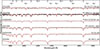 |
Fig. 1. Example spectral fits (red) to various hot subdwarfs (black) using the pipeline described in Sect. 4. Table 1 provides more details about the spectra. |
In total, our spectroscopic dataset study includes 3226 spectra for 253 single-lined hot subdwarf stars where each source has at least three spectra suitable for both atmospheric analysis and vrad determination. The spectroscopic data were reduced either using PyRAF procedures (Science Software Branch at STScI 2012), a python-based implementation of IRAF (Image Reduction and Analysis Facility; Tody 1986) which is a general purpose software developed by the National Optical Astronomy Observatories (NOAO), the MOLLY package (Marsh 1989, 2019), or instrument-specific pipelines. All methods include basic bias and flat-field corrections and wavelength calibrations.
3.2. Revised spectroscopic classifications
The classification scheme used in Paper I was based on the scheme outlined in Moehler et al. (1990), which was updated and extended to incorporate a wider range of spectroscopic classes (see Paper I for details). It was based on visual inspection and is adopted in this work. In addition to the basic spectral classes of sdB, sdOB, sdO, and He-sdO, here we also incorporate intermediate helium-sdOBs (iHe-sdOB), and extreme helium-sdOs (eHe-sdO) into our scheme, as already adopted in other works (Luo et al. 2021; Dorsch 2024; Geier et al. 2024). Visually, both iHe-sdOB and eHe-sdO stars exhibit strong neutral and ionised helium lines. However, eHe-sdO stars are characterised by weak or even absent hydrogen lines. We classify these subgroups based on their helium abundances derived from spectral fitting. We define iHe-sdOB stars as those with helium abundances between log n(He)/n(H) = − 1.2 and log n(He)/n(H) = 0.6, while stars with log n(He)/n(H) > 0.6 are classified as eHe-sdO. The divisional point of the helium-enriched stars is motivated by a clear gap that is seen in the log n(He)/n(H)−Teff parameter space at log n(He)/n(H) = − 1.2 (e.g. see Fig. 3b). Lastly, we point out two misclassified systems in Paper I: [L92b]MarkA and TYC6017-419-1. These were classified as sdO and sdOB respectively. They have, however, been reassigned as eHe-sdOs herein. Table 2 includes the most accurate and current information.
Excerpt from the table of atmospheric parameters.
4. Atmospheric and stellar parameter determination
4.1. Model atmospheres and synthetic spectra
For the determination of the atmospheric parameters effective temperature (Teff), surface gravity (log g) and helium abundance (log n(He)/n(H)), we applied the same state-of-the-art set of model atmosphere grids (the second generation Bamberg model grids) to all hot subdwarf stars for a homogenous analysis (also used in Heber et al. 2025; Latour et al. 2026; Geier et al. 2024), which is detailed below. For each stellar spectrum we performed a full spectral fit. Spectra that did not cover the hydrogen Balmer jump (covering at least about 3700–5000 Å) were not considered in the atmospheric parameter determination, and only used for the radial velocity calculation. The same model grid was used for all stars, spanning 9000–75 000 K in Teff, 3.8–7.0 in log g, and −5.05 to +2.64 in log n(He)/n(H); regions beyond the Eddington limit (low log g at high Teff) are excluded. A hybrid non-local thermodynamic equilibrium (NLTE) approach was adopted to balance computational efficiency with the need to capture NLTE effects in hot early-type stars. Synthetic spectra were generated with the ATLAS12, DETAIL, and SURFACE (ADS) codes, as in previous hot subdwarf studies (Latour et al. 2018b; Schneider et al. 2018; Geier et al. 2024). Specifically, ATLAS12 (Kurucz 1996) computed the LTE temperature and (electron) density stratifications; DETAIL (Giddings 1980) solved the radiative transfer and rate equations for hydrogen and helium populations, iteratively feeding corrections back into ATLAS12 (Irrgang et al. 2018); and SURFACE (Giddings 1980) produced the final synthetic spectra including line broadening.
The model fits were carried out using the Interactive Spectral Interpretation System (ISIS; Houck & Denicola 2000), employing a χ2-minimisation technique to perform a global fit across the entire usable spectral range. A detailed description of the implementation of spectral fits in ISIS can be found in Irrgang (2014). The routine was automated such that the fits could be done in parallel, and takes about two hours to complete in total for our sample of 253 single-lined hot subdwarfs on a multi-core cluster.
In the automated spectroscopic fitting procedure, the continuum is modelled with an Akima spline (Akima 1970), which is anchored at 100 Å intervals while avoiding the hydrogen and helium absorption features in the spectrum. The atmospheric parameters Teff, log g, and He-abundance are fitted simultaneously with the continuum, in addition to the radial velocity. Poorly fitting spectral regions are automatically excluded. For targets with multiple spectroscopic observations, each individual spectrum was fit separately. This method is the same as that used in Heber et al. (2025) and Latour et al. (2026).
For the atmospheric parameters Teff, log g, and log n(He)/n(H), and their associated statistical uncertainties, we adopted weighted averages, where each measurement was weighted by the square of the effective signal-to-noise ratio (S/Neff) of the corresponding spectrum – that is, an inverse-variance weighting. The S/Neff values were computed after rescaling the flux uncertainties such that the reduced χ2 = 1 for each spectral fit. This approach assigns greater weight to higher-quality spectra while preventing spectra with more data points from being overrepresented in the combined values.
The spectral resolution for each fit is set by the average full-width at half-maximum (FWHM) of the arc lamp emission lines, which reflects the instrumental broadening of the spectrograph, or taken from archival values when available. Each fit was then visually inspected to assess its quality. Spectra with S/N < 5 were discarded. In cases where poor wavelength calibration was detected during visual inspection, efforts were made to reprocess the data to obtain a usable spectrum; if re-reduction was unsuccessful, the spectrum was excluded from the fitting routine.
The routine was performed twice: first with the projected rotation vrot sin i constrained to values below 30 km s−1 typical for hot subdwarf stars (Geier & Heber 2012) and then with vrot sin i treated as a free parameter to enable the detection of rare, rapidly rotating hot subdwarfs. No such candidates were identified using the high-resolution data. In total, the routine produced 3226 reliable spectroscopic fits after 88 were discarded due to poor quality. The results with vrot sin i constrained below 30 km s−1 were used to ensure reliable log g estimates, thus avoiding the correlation between vrot sin i and log g.
4.2. Systematic uncertainties
Our automated and homogenous spectral analysis approach is intended to minimise internal systematic uncertainties that would be introduced by the use of multiple model grids or fit methods. However, other aspects of data handling contribute to further uncertainty. Next to the formal uncertainty caused by statistical noise, we identify and characterise systematic uncertainties that arise from three main sources: (1) variability introduced by data reduction and observing conditions (e.g. clouds), (2) calibration offsets between different instruments and observing setups, and (3) the choice of metallicity used in the spectral fitting procedure. In the following we detail these systematic uncertainties.
Since our spectral fits were performed independently for each spectrum, we can directly assess the repeatability of parameter estimates under similar conditions. The majority of our spectra were obtained with the INT/IDS instrument using the 1200B setup (see Table 1), which covers the full optical range except for Hα. For each star with at least three INT spectra at S/Neff > 25, we computed the one-sigma observed scatter in Teff, log g, and log n(He)/n(H) around their respective weighted means. By comparing this observed scatter to that expected from formal uncertainties, we isolate the intrinsic scatter likely associated with data reduction and observing conditions. This contribution amounts to, on average, 0.55% in Teff, 0.039 in log g, and 0.02 in log n(He)/n(H). More precisely, the contribution is a function of Teff as presented by a light dashed-blue polynomial in each panel of Fig. 2, and labelled as the intrinsic scatter.
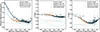 |
Fig. 2. Three-panel figure showing our best estimates of the overall uncertainties in Teff, log g, and log n(He)/n(H) (from left to right), displayed as scattered markers. The Teff uncertainties are plotted as fractional values (ΔTeff/Teff, i.e. 1–5%). Helium-rich and helium-poor stars are separated and indicated as orange squares and dark blue circles, respectively. The solid orange and dark blue lines are polynomial fits (Equation (1)) to these scattered markers, and the coefficients of these are given in Table A.2. The dashed polynomials represent the identified uncertainty contributions from the intrinsic scatter measured in our INT data and from the metallicity abundance uncertainty, as described in Sect. 4.2. The formal statistical errors are given by the error bars of the scattered markers and the instrumental offset between INT and ALFOSC is given by a black-dashed line. All four identified uncertainties are added together in quadrature to arrive at the uncertainties used for the analysis in this work. |
The largest set of overlapping observations between different instruments occurred for nine stars observed with both INT and ALFOSC (150 spectra between them in total). To estimate systematic offsets in Teff, log g, and log n(He)/n(H) between the two setups, we first computed uncertainty-weighted mean values and associated errors for each star from each instrument. The per-star differences were then modelled using a maximum likelihood approach that fits simultaneously for a constant systematic offset and an additional intrinsic scatter term beyond the reported statistical uncertainties. This method provides an unbiased estimate of the systematic offset while accounting for excess variance not captured by formal errors. The resulting absolute systematic offsets are 0.81 ± 0.13% in Teff, 0.04 ± 0.01 in log g and 0.03 ± 0.01 in log n(He)/n(H), which are global offsets which we take as a proxy to represent the uncertainties that arise from using different instruments. These are given as horizontal dotted-black lines in Fig. 2 and are labelled as the instrumental offset. It is important to emphasise, however, that adopting a single offset derived from INT and ALFOSC as representative of all instrumental pairings in our programme is a strong simplification. Intrinsic differences between spectrographs cannot, in general, be encapsulated by a universal correction. We underscore that our adopted offsets are tailored to this specific comparison, and any assumed cross-instrument calibration should be evaluated with care for the instruments and samples at hand.
All atmospheric parameters presented in this study are based on fits assuming standard sdB atmospheric metallicity (log z/zsdB = 0; using abundances from Pereira 2011). Accurate measurements of atmospheric metallicity typically require high-quality ultraviolet (UV) data, which is available for only a limited number of hot subdwarf stars. Due to the opacity from numerous iron-group elements in the far-UV to extreme-UV range, the metallicity significantly affects the derived atmospheric parameters. The iron abundance serves as an indicator of this metallicity; it scatters with a standard deviation of 0.3 dex in the sample of Geier (2013). To account for this, we repeated the entire fitting routine for all stars with fixed metallicities of log z/zsdB = +0.3 and log z/zsdB = −0.3 (see also Heber et al. 2025). This variation leads to systematic uncertainties as a function of Teff, given by the dot-dashed polynomials in Fig. 2. In this case, since we fit all stars in the sample and have ample number statistics, we separate the stars into helium-poor and helium-rich objects, which returns a distinct behaviour for each group. For further visualisation of the impact of metallicity in the log g − Teff and log n(He)/n(H)−Teff parameter spaces, see Fig. A.1.
To derive the final systematic uncertainties on Teff, log g, and log n(He)/n(H), we combined the three isolated systematic uncertainties detailed above in quadrature, which results in the scatter markers in each panel of Fig. 2. To the total uncertainties in Fig. 2, we fit a third-order polynomial of the form
 (1)
(1)
where the best-fit coefficients for each parameter Teff, log g, and log n(He)/n(H) for both helium-poor and helium-rich objects are provided in Table A.2. Note that the formal statistical uncertainties are not included in these fits but are shown separately as error bars, allowing our estimates of the systematic uncertainties to be used independently in other works. In this paper, however, we combine the statistical uncertainties with the three systematic uncertainties described above in quadrature, and use these combined values for the remainder of the analysis. These represent our best estimates of the total uncertainty in the atmospheric parameters, incorporating both random and systematic sources of error.
4.3. Spectral energy distributions and stellar parameters
For the single-lined hot subdwarf stars in our sample, we applied the spectral energy distribution (SED) fitting routine first described in Heber et al. (2018), and in more detail in Section 2.2 of Dorsch (2024). This method compares apparent multi-band magnitudes collected from the literature though the VizieR database3 with synthetic SEDs, while keeping the stellar parameters fixed to the spectroscopically determined values. We refer the reader to Culpan et al. (2024) for a list of all the photometric catalogues queried. Interstellar extinction was modelled using the prescription of Fitzpatrick et al. (2019), adopting a standard extinction coefficient of R(55) = 3.02. Inspection of the SED further allows us to detect the presence of an IR-excess, which is visible if a cool MS companion is bright enough to emit more IR flux than the primary hot subdwarf star. While Paper I identified 48 out of the 305 hot subdwarfs in the 500 pc sample to likely harbour F, G, or K-type MS companions, a re-analysis of the SED fits identified a further nine of the 253 single-lined systems as showing a hint of IR excess, indicative of a cool companion star (see Table A.1 for a list of these objects). Because the small amount of IR flux in these systems has little to no effect on the derived atmospheric parameters from the optical spectra, they are included in our spectroscopic analysis; other composite-colour binaries were excluded. In the case of the SED fits, the flux contribution of the companion was modelled using the PHOENIX Göttingen spectral library (Husser et al. 2013)4. All SED fits were constrained using the atmospheric parameters from our spectroscopic fits (Teff, log g, and He-abundance) along with their corresponding systematic uncertainties (Sect. 4.2). Thanks to the precise parallax measurements from the Gaia space mission (Gaia Collaboration 2023), the interstellar reddening can be constrained, which allows absolute stellar radii R, luminosities L, and masses M to be determined with high accuracy and minimal systematic uncertainties, particularly for our sample of nearby objects, which are evaluated using the following relations:
 (2)
(2)
where θ is the angular diameter, ϖ is the parallax, and G is the gravitational constant.
We employed a Monte Carlo method to assess the uncertainties in our calculations. The input spectroscopic parameters, Gaia parallax, and angular diameter were represented by Gaussian distributions. For each star, 106 samples were generated, with each array carried through the full calculation to the final derived parameter. The masses and luminosities listed in Table 3 are the median values of these distributions, while the asymmetric uncertainties are defined by the 84th and 16th percentiles, corresponding to the 68% confidence interval around the median mass. We refer to these masses and luminosities, which can be constrained primarily due to the Gaia parallax, as parallax-based masses and parallax-based luminosities for simplicity.
Excerpt from the table of SED and HRD parameters.
5. Kinematical method and population assignment
Hot subdwarf stars are found across all Galactic stellar populations. For less evolved stars, chemical tagging provides a powerful means of identifying stellar population membership (see Bland-Hawthorn & Gerhard 2016, for a full review). In hot subdwarf stars, however, strong diffusive processes in their atmospheres significantly modify the abundance patterns, rendering chemical tagging ineffective (Michaud et al. 2011). As a result, population studies of hot subdwarfs must instead rely on kinematical analysis, which requires complete 6D phase-space information (Pauli et al. 2006). From Gaia we have accurate positions, parallaxes, and proper motions for all stars in our sample. The final parameter, vrad, is straightforward in principle but observationally intensive, especially given that a large fraction of hot subdwarfs that reside in close binaries exhibit velocity variations of hundreds of km s−1 and their orbital motion needs to be corrected for to obtain the radial component of the space velocity (Maxted et al. 2001; Napiwotzki et al. 2004; Copperwheat et al. 2011; Geier et al. 2022; Schaffenroth et al. 2022).
5.1. Radial velocities
All available spectra were processed with our automated fitting pipeline (Sect. 4) where the vrad is an output of the full model fit. These are then corrected to the heliocentric frame. For known close binaries, we adopt systemic velocities from the literature. For ∼30 systems solved in this work, we use systemic velocities derived from orbital solutions (Dawson et al. in prep.). For apparently non-variable or unsolved systems, we take the mean vrad of the maximum and minimum vrad values from the fitted spectra. This was chosen because of the poor orbital coverage for some binary systems. The standard deviation of these measurements is used as the uncertainty on the systemic radial velocity. Finally, systematic uncertainties were estimated for each instrumental setup and are listed in Table 1. Where available, we used the root mean square of the wavelength calibration derived during data reduction. For setups lacking direct calibration data, we estimated systematic uncertainties from the typical deviations of radial velocities measured for vrad-standard stars throughout the observing programme. These systematic contributions were then added in quadrature to the statistical uncertainties to obtain the final error estimates.
5.2. Kinematics
We compute the Galactic rest frame velocity components U, V, and W, defined as positive towards the Galactic Centre, the direction of Galactic rotation, and the north Galactic pole, respectively. These velocities are derived directly from each star’s vrad, distance, position, and proper motion as provided by Gaia, without assuming a specific Galactic potential or computing stellar orbits (see Johnson & Soderblom 1987, for details). Distances were calculated by inverting the zero-point–corrected Gaia parallaxes, with the parallax uncertainties inflated following El-Badry et al. (2021). Velocities are transformed into the Galactocentric frame, adopting a solar distance from the Galactic centre r⊙ = 8.4 kpc and a circular velocity of the local standard of rest (LSR) of VLSR = 242 km s−1 following the best-fit model of Irrgang et al. (2013). The solar velocities with respect to the LSR were assumed to be (U⊙, V⊙, W⊙) = (11.1, 12.2, 7.3) km s−1 based on the results of Schönrich et al. (2010).
Population membership is assigned probabilistically in UVW space using a Gaussian mixture model (GMM) with three fixed components (thin disk, thick disk, halo). The velocity ellipsoid centroids, dispersions, and correlations are adopted from Anguiano et al. (2020), while only the relative weights of the components are optimised using an expectation-maximisation (EM) algorithm. The standard EM-GMM framework (Dempster et al. 1977; McLachlan & Peel 2000) provides a probabilistic decomposition of the data into a set of Gaussian components, but assumes error-free measurements, treating all observed scatter as intrinsic population variance. Our approach explicitly incorporates the per-object covariance matrix of the measurement errors into both the expectation and maximisation steps, following the extreme deconvolution methodology (Bovy et al. 2011), which has been widely applied to astronomical data with heteroscedastic uncertainties (Hogg et al. 2010; Kelly 2007).
6. Results
Tables 2, 3, and 4 summarise the results of our spectroscopic, photometric, and kinematic analyses, respectively. Table 2 lists the atmospheric parameters derived from our spectroscopic fits, including Teff, log g, helium abundance, and systemic radial velocity. The stated uncertainties on the atmospheric parameters correspond to the systematic uncertainties derived in Sect. 4.2, while those on the systemic radial velocities also include the σvrad values provided in Table 1. Table 3 presents the parameters obtained from our SED fitting, such as parallax-based masses, luminosities, radii, and interstellar extinction. The final columns of this table also report the theoretical masses and evolutionary lifetimes inferred from our interpolation routine (see Sect. 7.1). Finally, Table 4 provides the results of our kinematical analysis, listing the Galactic velocity components (U, V, W) and the corresponding probabilities of membership in the thin disk, thick disk, and halo populations. In this paper, we continue to divide our stars into groups based on the visual inspection classification scheme described in Paper I with the addition of intermediate and extreme helium classes, in order to maintain consistency. Five objects (GALEX J19498-2806, GALEX J191509.0-290311, HD 319179, CD-39 14181, and EC 21494-7018) have spectra of insufficient quality to be modelled reliably. For completeness, we nevertheless provide their atmospheric, kinematic, and stellar parameters, assigning a quality flag of ‘B’ in all three tables; reliable parameters are indicated by a flag of ‘A’. These five objects were excluded from the mass distribution analysis presented in Sect. 6.4.
Excerpt from the table of kinematic and membership parameters.
6.1. Effective temperature and surface gravity
The distribution of our 253 single-lined hot subdwarf stars in the effective temperature – surface gravity plane (hereafter Kiel diagram) is displayed in Fig. 3a where the different spectral classes (see Sect. 3.2 and paper I) are colour-coded accordingly. The light-blue region encapsulates the EHB between the zero-age EHB (ZAEHB) at core helium ignition and the terminal-age EHB (TAEHB; Dorman et al. 1993) both for solar metallicity. The zero-age helium-burning main sequence (He-MS; Paczyński 1971) is given as a dashed-grey line. Three post-EHB evolutionary tracks from Han et al. (2002) are shown in black for the same core mass of 0.45 M⊙ with envelope masses of 0.0, 0.001, and 0.005 M⊙, where the thickness of the line is proportional to the timescale. A double He-WD merger track from Zhang & Jeffery (2012) for two 0.3 M⊙ WDs is given as a orange dot-dashed line. TYC 6800-72-1 appears to lie high on this track; however, it is unlikely to be physically associated with it, as it exhibits radial-velocity variations indicative of a close compact companion and is the only helium-enriched object in our sample with a detected companion (Dawson et al. in prep.).
In Fig. 3a, most sdB and sdOB stars (blue stars and green diamonds, respectively) lie in a well-defined region between the ZAEHB and the TAEHB. Most sdBs appear to cluster where the EHB evolutionary tracks predict the longest timescale near the ZAEHB, giving rise to a dearth of sdBs near the TAEHB. The sdOBs predominantly reside at hotter temperatures (Teff > 30 000 K) and higher surface gravities (log g > 5.5). Nearly all of the eHe-sdOs, given by the filled orange circles, are located above the TAEHB and the He-MS, hinting at under-estimated surface gravities, though they align well with the He-WD merger track. Other large-sample studies of hot subdwarfs (e.g. Stroeer et al. 2007; Latour et al. 2014; Fontaine et al. 2014; Németh et al. 2012; Luo et al. 2019, 2021; Lei et al. 2018) have found substantial scatter in log g around the He-MS. This scatter likely arises from the challenges inherent in modelling helium-enriched atmospheres, and highlights the need for improved atmospheric models next to homogeneous analysis techniques to resolve these differences. The hydrogen-rich sdOs (purple triangles) are primarily situated below the He-MS at higher temperatures. Their position aligns well with post-EHB tracks, reinforcing a connection to the sdB stars.
6.2. Helium abundance
Figure 3b shows that our sample follows the helium patterns reported in previous studies (Edelmann et al. 2003; Németh et al. 2012; Luo et al. 2016; Lei et al. 2018), with two branches of He-poor stars exhibiting increasing helium abundance towards higher Teff. The empirical relations from Németh et al. (2012) and Edelmann et al. (2003) are included for reference as dashed black and red lines, respectively. The upper branch in our sample agrees reasonably well with the relation of Edelmann et al. (2003), but their lower branch is not clearly reproduced. In addition, most of our He-weak sdO stars lie below the relation reported by Németh et al. (2012), but are of similar abundance to most of the sdB and sdOB stars. Dashed-horizontal lines mark the log n(He)/n(H) = − 1.2 and log n(He)/n(H) = + 0.6 which we use to distinguish the iHe-sdOBs and the eHe-sdOB stars. A clear gap is seen at log n(He)/n(H) = − 1.2 but not for log n(He)/n(H) = + 0.6. Our sample contains one iHe-sdB (CPD-20 1123; Vennes et al. 2007), which is marked as a black circle in the diagram; another peculiar star is the well-studied BD+75 325 (Gould et al. 1957) as the only iHe-sdO in our sample.
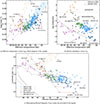 |
Fig. 3. Upper left: Teff − log g diagram of the hot subdwarf stars in the 500 pc sample, colour-coded as shown in the legend (lower panel). Three post-EHB evolutionary tracks for three different envelope masses from Han et al. (2003) are given as solid-black lines: 0.00, 0.001, and 0.005 M⊙ from bottom to top (Mtotal = 0.45 M⊙). The thickness of the lines are linearly proportional to the predicted evolutionary time. A double He-WD merger track from Zhang & Jeffery (2012) is shown as a orange dot-dashed line. The region encapsulated by the zero-age EHB and the terminal-age EHB from Dorman et al. (1993) is depicted as a shaded light-blue region which extends down to the He-MS from Paczyński (1971) which is shown as a dotted-grey line. All tracks are given for solar metallicity. Upper right: helium abundance – Teff diagram for the same stars. The helium sequences identified in earlier studies (Edelmann et al. 2003; Németh et al. 2012; Luo et al. 2016; Lei et al. 2018) are shown. Bottom: Hertzsprung-Russell diagram with the same hot subdwarf classes and evolutionary tracks as shown in the upper left panel. The He-MS from Paczyński (1971) is again shown as a dotted-grey line with the corresponding masses annotated. The horizontal dashed-black lines indicate the solar metallicity ZAEHB at log L/L⊙ = 1.05 at the start of the 0.45 M⊙ evolutionary tracks from Han et al. (2002), and the TAEHB of these tracks at the point of core helium depletion. Two additional ZAEHB positions are marked as dashed-red lines for the 0.40 M⊙ and 0.35 M⊙ evolutionary tracks to compare with the low-luminosity objects. Black pentagons mark the underluminous hot subdwarfs (log L/L⊙ < 1.05) in all three plots. Crimson pentagons indicate the three identified hot and helium-poor stars. The grey star marks the previous position of HD 188112. |
Németh et al. (2012) further discovered that hot subdwarfs predominantly cluster into two distinct groups within both the Teff − log g and Teff − log n(He)/n(H) diagrams. They inferred the presence of two characteristic hydrogen envelopes, each with differing masses and compositions. However, no clear gap is seen in our sample.
6.3. Stellar parameters and the HRD
The Kiel diagram provides useful information on the evolutionary stages and relative positions of stars in our sample. By combining this with precise parallax measurements from Gaia, we can compute stellar luminosities and construct a HRD, which allows for a more accurate characterisation of the stellar population thanks to precise luminosities. In Fig. 3c, the HRD of our sample is shown, including the same evolutionary tracks, EHB, and He-MS features highlighted in Fig. 3a.
Most sdB and sdOB stars are well situated in a narrow luminosity band between log L/L⊙ = 1.0 and 1.5, which implies that they are in a core helium burning stage. The horizontal dashed black lines indicate the solar metallicity zero-age EHB at log L/L⊙ = 1.05 at the start of the 0.45 M⊙ evolutionary tracks, and the point of core helium depletion for the same tracks. A few stars show much higher luminosities and are likely in a helium shell burning stage, such as the well-known post-HB star HD 76431 (Ramspeck et al. 2001; Khalack et al. 2014), as annotated in the plot, or are evolving towards the EHB. All helium-enriched hot subdwarfs in our sample are remarkably close to the zero-age He-MS of Paczyński (1971), irrespective of whether they belong to the iHe or eHe class, suggesting that most are in a core-helium burning phase.
Notably, excluding three objects with high re-normalised unit weight error values from Gaia (RUWE; Sect. 6.5), as well as the pre-ELM candidates CPD-20 1123 and EVR-CB-001 (see Sect. 6.3.1), 22 sdB stars are underluminous and are located below the canonical EHB in both the Kiel and HR diagrams (Figs. 3a, 3c), corresponding to a ratio of 0.10 ± 0.02 (binomial uncertainty) relative to the number of stars on the EHB band (sdB+sdOB). These stars are marked with black pentagons in all three plots (Fig. 3) for comparison. Interestingly, around half of these objects have exceptionally low helium abundances (log n(He)/n(H)≤ − 3.8; also seen by Latour et al. 2026), similar to the sdB closest to the Sun, HD 188112, which is also annotated in Fig. 3. These stars are classified as sdBs because their spectra are void of ionised helium lines upon visual inspection. Most have cooler temperatures and lower helium abundances than those identified in this region previously by Edelmann et al. (2003), whose trends marked with dashed-red lines do not extend to log n(He)/n(H)≤ − 3.8.
6.3.1. Underluminous hot subdwarfs
The physical origin of the underluminous population in our sample remains uncertain. These stars are located below the EHB and exhibit systematically higher surface gravities at a given effective temperature compared with the bulk of the sdB population. The horizontal red-dashed lines in Fig. 3c mark the ZAEHB for the 0.40 M⊙ and 0.35 M⊙ evolutionary tracks from Han et al. (2002). We find that these stars are likely associated with these low-mass tracks and discuss this further in Sect. 7.1.
We define ‘below-EHB’ objects as those with log(L/L⊙)≤1.05, based on the solar-metallicity 0.45 M⊙ EHB tracks of Han et al. (2002), which is appropriate given the local nature of our sample. The below-EHB population have been identified previously (e.g. Geier et al. 2022; He et al. 2025), though differ subtly in the criterion used to define them. At log L/L⊙ ≤ 1.05, we also observe a sharp drop in the luminosity distribution of the sdB and sdOB stars (Fig. 5), marking the possible transition to the low-mass hot subdwarfs, formed by non-degenerate helium ignition (e.g. Arancibia-Rojas et al. 2024). More discussion on the link between the low-luminosity stars and their low-mass is presented in Sect. 7.3.
Other observational studies in the literature generally define the EHB using metal-poor 0.47 M⊙ evolutionary tracks, such as those of Han et al. (2002) or Dorman et al. (1993). These tracks lie at higher luminosities in the HRD compared to the ZAEHB shown in Fig. 3c. This difference arises because metal-poor stars have lower opacities, allowing their cores to cool more efficiently. As a result, a larger amount of helium must accumulate before ignition, leading to a more massive core, a condition that also holds for more massive progenitors (MZAMS ≥ 2.0 M⊙; Arancibia-Rojas et al. 2024). If metal-poor tracks were adopted here, the proportion of below-EHB objects in our sample would thus be even higher. Another consideration is that the masses at the ZAEHB depend on the physics assumed in the models, such as overshooting prescriptions (see e.g. Ostrowski et al. 2021; Xiong et al. 2017, for more details).
Among the underluminous hot subdwarfs is HD 188112, regarded as the prototype sdB extremely low-mass (ELM) white dwarf progenitor (Heber et al. 2003) and the closest object in our sample to the Sun at just 71 pc. As already pointed out in Sect. 4.2, metallicity has an impact on the derived atmospheric and stellar parameters. Because Latour et al. (2016) analysed UV data, HD 188122 has a well-determined abundance pattern, which turns out to be metal-poor. This pattern is well represented by log z/zsdB = −1, which we adopted to derive Teff = 21650 ± 350 K and log g = 5.81 ± 0.07 for HD 188112 from a very high S/N WHT/ISIS spectrum displayed in Fig. 1. In particular log g is higher than derived in the study of Heber et al. (2003) which gave Teff = 21 500 ± 500 K and log g = 5.66 ± 0.05. The difference in log g can be traced back to a combination of different model atmospheres used at the time (see Heber et al. 2000), and the wavelength coverage of the spectra analysed. Notably, the TWIN spectra analysed in Heber et al. (2003) do not adequately cover the hydrogen Balmer jump, which is crucial for accurate log g determination. The updated parameters are shown in the Kiel (Fig. 3a) and HR (Fig. 3c) diagrams, with the revised position of HD 188112 indicated by a light dashed-grey line, and its previous location is marked with a grey star. Because its effective temperature is essentially unchanged, its HRD position remains the same. In this diagram, the star lies very close to the low-mass sdB (0.35 M⊙) tracks of Han et al. (2002). Given the higher log g found in this work, the mass derived from the SED and parallax is 0.33 M⊙, substantially higher than the previously inferred 0.24 M⊙ (Heber et al. 2003), but in excellent agreement with the evolutionary tracks. Hence, we find it very likely that HD 188112 is not an ELM progenitor as previously thought, but among the least massive EHB stars identified in this sample. TYC 5417-2552-1 (annotated in Fig. 3) has very similar atmospheric and stellar properties to HD 188112. We find TYC 5417-2552-1 has a mass of  which aligns well with the low-mass tracks of Han et al. (2003) and is therefore also likely a low-mass sdB rather than an ELM progenitor as proposed by Kawka et al. (2015).
CPD-20 123 is the only identified iHe-sdB star within the 500 pc sample and is marked with a black circle in Fig. 3. This object has previously been interpreted as a post-common-envelope binary evolving towards the EHB, likely hosting either a WD or dM companion on a 2.3 day orbital period (Naslim et al. 2012; Kupfer et al. 2015). However, our analysis yields a substantially lower mass for the hot subdwarf than assumed in these studies,  M⊙, based on its atmospheric parameters (Teff = 21610 ± 350 K and log g = 5.04 ± 0.04) and the Gaia parallax. This suggests that CPD-20 1123 might instead be a pre-ELM object evolving towards the white dwarf cooling track, rather than an EHB progenitor. The system may thus be similar to the pre-ELM + He-WD system EVR-CB-001 (Ratzloff et al. 2019), which is also part of the 500 pc sample; in this case our mass (
 M⊙) is somewhat higher than the previously published value (
 M⊙), but still consistent with a pre-ELM nature. Both TYC 5417-2552-1 and CPD-20 123 are removed from subsequent analysis.
6.3.2. Hot and helium-poor sdBs
Three stars with helium abundances below log n(He)/n(H) < − 3.8 (UCAC4 314-235772, PG 1538+401, and TYC 4651-1475-1) lie between 35 000 and 40 000 K, a temperature region of extreme helium abundance diversity in hot subdwarf stars. These objects show no evidence of ionised or neutral helium in their atmospheres, and are therefore also classified as sdBs despite having effective temperatures close to the coolest sdO stars. In Fig. 3, they are distinguished with crimson pentagons and unlike the cool sdBs with log n(He)/n(H) < − 3.8 discussed above, are located above the ZAEHB in both Figs. 3a and 3c, consistent with an evolved state. This may hint at a possible evolutionary connection between the cool helium-poor sdBs and the helium-poor sdOs.
Median masses and luminosities from the SED and HRD.
6.4. Mass and luminosity distributions
Our results from the SED fitting routine detailed in Sect. 4.3 combined with Gaia DR3 parallaxes are used to calculate the median masses and luminosities for each spectral class and are listed in Table 5. The distribution of masses as a function of Teff is shown in Fig. 4, where the black shaded area highlights ± 0.05 M⊙ around a mass of 0.47 M⊙. The pink-shaded region extends this further down to 0.35 M⊙, which is the minimum core mass covered by the evolutionary tracks of Han et al. (2002). Our results are further presented as mass and luminosity distributions in Fig. 5, shown as normalised Kernel Density Estimates (KDEs) for a clear comparison between sub-classes. A KDE is a smoothed representation of the distribution, where each data point contributes a small Gaussian kernel; the sum of these kernels gives a continuous estimate of the probability density. The smoothing bandwidth is 0.05 M⊙ in all cases which sets the scale over which individual measurements contribute to the distribution. The uncertainties are derived directly from simple Monte Carlo arrays, with asymmetry reflecting the 16th and 84th percentiles. For the full sample (flag ‘A’ in Table 3) of 243 single-lined stars (grey line; central panel of Fig. 5), we derive a median mass of M = 0.48−0.01+0.14 M⊙, which is within the range of previous studies (∼0.46 − 0.5 M⊙ Fontaine et al. 2012; Schaffenroth et al. 2022), depending upon metallicity and evolutionary model prescriptions (see Sweigart & Gross 1978; Cassisi et al. 2016; Arancibia-Rojas et al. 2024, and references therein).
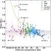 |
Fig. 4. Distribution of our stars in the mass – effective temperature plane. The He-MS (Paczyński 1971) is shown as a dashed grey line. The grey-shaded band is centred on a mass of 0.47 M⊙ and spans ±0.05 M⊙, corresponding to our mean uncertainties. The pink-shaded region extends down to 0.35 M⊙, the minimum core mass predicted by the evolutionary tracks of Han et al. (2002). Pentagons indicate the same stars as in Fig. 3. |
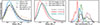 |
Fig. 5. KDE representation of the mass and luminosity distributions for the full sample and subgroups of hot subdwarf stars. Uncertainties are not included in the KDEs, allowing clearer comparison between different hot subdwarf classes. |
Lei et al. (2023b) analysed the mass distributions of 667 single-lined hot subdwarf stars observed with LAMOST, dividing them into three groups based on parallax uncertainty (see their Table 2). For comparison with the 500 pc sample, their group 3 is most relevant, both in terms of sample size and parallax precision (better than 5%). Their overall mean mass of 0.48 M⊙ agrees with our median result of 0.48 M⊙. Similar agreement is found for He-rich hot subdwarfs, which show a relatively lower peak mean mass than expected (Han et al. 2003) of 0.5 M⊙ in both studies, highlighting the need for improved modelling of the ionised helium-dominated atmospheres. However, a notable discrepancy exists for the hydrogen-rich sdO stars: Lei et al. (2023b) report a mean of 0.36 M⊙, significantly lower than our 0.50 M⊙, which is unexpected given the likely evolutionary connection between sdB and sdO stars.
6.5. Low-mass hot subdwarfs
The central panel of Fig. 5 shows the mass distribution of underluminous sdB stars located below the EHB in the HRD (22 stars; log L/L⊙ < 1.05) in red compared to the sdB, sdOB, and sdO stars above the EHB (189 stars; log L/L⊙ > 1.05) in teal. The below-EHB objects show an offset, peaking at M = 0.43−0.09+0.11 M⊙. Lei et al. (2023b) noted that large parallax uncertainties (up to about 20%) can bias samples towards low-mass objects, likely due to systematic Gaia effects at greater distances. Our sample is largely unaffected, with a mean parallax uncertainty of only 1.54%. The exceptions are EC 20106-5248, PG 1634+061, and RL 105, with parallax uncertainties of 3–6% and high RUWE values (2–3). Their parallax-derived masses fall below 0.4 M⊙ and are likely unreliable due to poor Gaia astrometry, while their spectroscopic surface gravities place them on the EHB and should not be affected. Their stellar parameters are provided in Tables 3 and 4 with the flag ‘B’, but are excluded from the mass distribution and HRD analysis in this paper.
To evaluate the statistical significance of the low-mass peak observed for our underluminous hot subdwarfs, we apply a two-sample Kolmogorov-Smirnov (KS) test, supplemented by the Mann-Whitney U test as a complementary check, both implemented through the SciPy Python module. The underluminous population are compared against those classed as sdB, sdOB, and sdO with log L/L⊙ > 1.05 (helium-rich objects are excluded). We accounted for measurement uncertainties in the parallax-derived masses using Monte Carlo resampling. In 10 000 trials, each star’s mass was randomly varied within its uncertainty, and the statistical tests were repeated. Both the KS and Mann–Whitney tests consistently yielded low p-values (median pKS ∼ 0.02, pMW ∼ 0.007), rejecting the possibility that the two samples share the same parent distribution with ∼99.5% confidence. This provides strong evidence that the underluminous stars have a different mass distribution from the general hot subdwarf population in our sample.
Kinematic population membership.
6.6. Population membership results
The results of our kinematical analysis (described in Sect. 5.2) are summarised in Table 6, and visualised in the U-, V-, and W-component diagrams, along with the Toomre diagram in Fig. 7. The pale-blue, dark-blue, and orange contours mark the 2σ contours of the thin disk, thick disk, and halo populations, respectively. For visual purposes, individual stars are coloured based on the Galactic component membership simply with the highest probability. In Table 4, these numbers therefore add up to more than the quoted membership fraction, which are calculated by summing up each membership probability given in Table 4. As expected for a local neighbourhood sample, the majority (86 ± 2%) of stars are classified as thin disk objects, while 13 ± 1% and 1 ± 1% are associated with the thick disk and halo, respectively. Notably, three of the four stars assigned to the halo population are helium-enriched, namely LS IV -14 116 (Randall et al. 2015), Feige 46 (Latour et al. 2019), and BD+39 3226 (Schindewolf 2018) and are previously known to belong to the halo. If eHe-sdOs are indeed post-merger objects, they are expected to be on average older owing to their formation delay time (see Figure 14 in Rodríguez-Segovia et al. 2025), and should therefore preferentially be in older Galactic populations and not in the young disk (Han 2008; Rodríguez-Segovia et al. 2025). The only helium-poor star in the halo, BD +48 2721, is a peculiar object with an identified 3He isotopic anomaly, and is likely a BHB star given its relatively low effective temperature (Schneider et al. 2018).
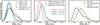 |
Fig. 6. Same KDEs as presented in Fig. 5, but using theoretical masses derived from our MCMC interpolation procedure in the HRD described in Sect. 7.1. Additionally, the right panel shows the estimated mass distributions of the He-rich stars derived by projecting each object to its nearest point along the He-MS (Paczyński 1971) in the HRD. |
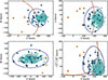 |
Fig. 7. Distribution of the 500 pc sample in the W-V, U-V, W-U, and Toomre (lower right) diagrams. The stars are marked as light blue circles, dark blue squares, and orange triangles to indicate thin disk, thick disk and halo membership, respectively. Two-sigma contours of the Galactic components are given in the same colour scheme. The position of the Sun is given by the black circle. |
Figure 8 presents the HRD for stars belonging to the thin disk, thick disk, and halo populations, arranged from left to right. The dashed-black line represents the solar ZAEHB at log L/L⊙ = 1.05 which we have used to define the underluminous hot subdwarfs (Sect. 6.3.1). A striking feature is the exclusive presence of underluminous hot subdwarfs within the Galactic thin disk population. While the ZAEHB is expected to shift to slightly higher luminosities in older, more metal-poor populations such as the thick disk and halo (Dorman et al. 1993), this trend alone does not account for the absence of such low-luminosity stars in those populations. We note that the thick disk and halo subsamples comprise only 22 and 4 stars, respectively, limiting the statistical power of this comparison. Under the null hypothesis that all populations share a common below-EHB fraction, the probability of observing zero below-EHB stars in the thick disk is p = 0.15 (binomial statistics), consistent with a ∼1σ statistical fluctuation, and the halo result is not statistically significant. However, similar studies of hot subdwarf populations with comparable sample sizes found smaller below-EHB fractions of 6% (Latour et al. 2026) and 0% (Heber et al. 2025), compared with 10% in our sample. Although these surveys are not volume-limited, their targets have larger average distances of 800 pc and 1500 pc, respectively, supporting the conclusion that the presence of below-EHB hot subdwarfs is linked to the age of the stellar population.
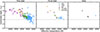 |
Fig. 8. Three-panel plot showing the HRDs for the thin disk, thick disk, and halo populations in our sample, as determined from our kinematic analysis in Sect. 5. The Solar-metallicity ZAEHB at L/L⊙ = 1.05 is overlaid to highlight that only objects associated with the thin disk population fall below the EHB. |
7. Discussion
7.1. Comparison to theoretical tracks
Accurate luminosities are available for all stars in our sample (see Sect. 4.3). This enables us to interpolate theoretical stellar masses from their positions in the HRD, which we can then directly compare with the masses obtained from the SED and parallax fitting. For simplicity, we relied on the evolutionary tracks from Han et al. (2002), which cover the EHB and early post-EHB evolution for core masses Mcore between 0.35 and 0.75 M⊙ and hydrogen-rich envelope masses Menvelope between 0 and 0.005 M⊙. Because the evolutionary tracks overlap considerably in the HRD, we used a Markov Chain Monte Carlo (MCMC) approach to explore the full range of possible age, core mass, and envelope mass combinations, and to predict log Teff and log L for each case. These predictions are compared to the spectroscopically derived effective temperature and parallax-luminosity within a multivariate normal likelihood function incorporating observational uncertainties and their covariance5. The log-likelihood function is given by
 (3)
(3)
which is probed by sampling the posterior probability distribution during the MCMC routine. Each χ2 is defined as
 (4)
(4)
 (5)
(5)
Since a given position in the HRD can correspond to multiple combinations of Mcore, Menvelope, and age, the resulting posterior parameters are often degenerate. To reduce this degeneracy and improve sampling efficiency, we impose priors informed by each object’s spectroscopic type. For the sdB stars, a prior proportional to the inverse of the evolutionary speed in the HRD was applied, favouring slower evolutionary phases. Conversely, for sdO stars, the prior is proportional to the evolutionary speed itself, thereby favouring faster evolutionary phases consistent with their likely post-EHB evolutionary status. A flat probability distribution was assumed for the sdOB stars as their specific evolutionary status is unclear. No other priors were applied.
The derived theoretical mass distributions are shown as KDEs of the entire posterior sample distribution in Fig. 6, where the central and left-most panels may be directly compared to the parallax-based mass distributions in Fig. 5 above. As shown in Table 5, both the HRD and parallax-based masses are in excellent agreement. Moreover, the below EHB objects shown as dashed-red lines in the central panels also agree well with each other, both exhibiting a pronounced peak that is lower compared with the full sample. Because luminosity can be measured more precisely than log g from spectroscopy, the theoretical masses exhibit narrower distributions. However, it should be noted that uncertainties in the evolutionary tracks themselves are not accounted for here.
The HRD-derived mass distribution seen for the sdOs is quite broad (0.41–0.65 M⊙; 68% confidence). This is caused by their position in the HRD at high luminosities and temperatures, where there is a large overlap between the high-mass and the evolved lower-mass tracks. This degeneracy was partially alleviated by imposing a prior that favours more evolved positions along the tracks, although in some cases younger and more massive solutions remain preferred. The uncertainties on our parallax-based masses for sdOs (approximately ±0.15 M⊙) again prevent a definitive resolution of this degeneracy.
7.2. Mass and luminosity distribution for He-sdO stars
In the case of the eHe-sdO and iHe-sdOB stars, both observational and theoretical masses lie within the range of what is expected for the scenario involving the merging of two He-WDs (0.4–0.7 M⊙; e.g. Webbink 1984; Saio & Jeffery 2000; Han et al. 2003). In particular, the HRD distribution of eHe-sdO masses (0.52−0.07+0.08 M⊙; Table 5) is very similar to the predictions of Han et al. (2003) for the merger channel (see their Figure 12; ≈ 0.54 ± 0.06 M⊙). The slightly wider mass range seen in our HRD masses might point to a wider range of masses of the double white dwarf binaries than assumed in Han et al. (2003), or hint at contribution from other merger scenarios. Note that the models of Han et al. (2003) did not consider helium-enriched envelopes and did not model the merger itself, limiting the accuracy of interpolated masses for He-rich stars.
The luminosity distribution of our eHe-sdO sample has a median of log(L/L⊙) = 1.88−0.23+0.24, which is broadly consistent with the predicted median for the hybrid CO+He WD merger channel (Justham et al. 2011). Our results somewhat favour the model variant in which approximately 0.1 M⊙ of the He-WD is not accreted. This finely tuned channel, involving mergers between post-sdB and He WDs, also predicts a high-luminosity tail up to log(L/L⊙)≈3.0, and almost no objects with log(L/L⊙) < 1.6. In contrast, only one star in our sample exceeds log(L/L⊙) > 2.5, while we observe a clear extension of sources down to log(L/L⊙)≈1.0. Although the absence of a pronounced high-luminosity wing could be attributed to small-number statistics (our sample contains only 15 eHe-sdOs), the low-luminosity tail is not reproduced by the models of Justham et al. (2011). Given that our sample includes a non-negligible fraction (∼10%) of low-mass, low-luminosity sdBs, this may offer a constraint on the input merger population for the models.
Our population of iHe-sdOBs divides into two distinct groups. The lower-luminosity objects coincide with the He-poor sdOBs, whereas the higher-luminosity objects are more closely associated with the eHe-sdOs in both the HR and Kiel diagrams. A similar division was also reported by Dorsch (2024) in their SED analysis of the spectroscopically identified hot-subdwarf sample of Culpan et al. (2022).
The evolutionary tracks of Han et al. (2002) were computed only for core masses up to 0.75 M⊙, and therefore may not cover several of the more luminous iHe-sdOB and eHe-sdO stars (see the proximity of these stars to the He-MS in the HRD in Fig. 3c). Since all our helium-rich objects lie close to the He-MS of Paczyński (1971) in the HRD, we estimated the masses of all He-rich stars in our sample by projecting their positions onto this sequence. The resulting mass distributions, shown in the right panel of Fig. 6 along with the interpolated masses from Han et al. (2002), estimate the iHe-sdOB stars to peak at 0.59−0.07+0.08 M⊙, while the eHe-sdO stars show a broader distribution between 0.55 and 0.85 M⊙ (68% range). These values are systematically higher than those inferred from the parallax in the SED method and the Han et al. (2002) tracks, and would therefore require the progenitor population of close double white dwarfs to span a similarly broad mass range. For TYC 5720-292-1 (annotated in Fig. 4), the parallax-based and He-MS masses are in good agreement; however, for BD+39 3226, the He-MS mass is about 0.3 M⊙ lower.
7.3. Intermediate-mass progenitors
Hot subdwarfs are commonly discussed in the canonical framework of low-mass progenitors (about 0.7 − 1.8 M⊙), in which helium ignition occurs via a core flash at a mass of roughly half a solar mass. This picture is supported by a corresponding peak in the observed mass distribution (Schaffenroth et al. 2022; Lei et al. 2023b, also Sect. 6.4). Intermediate-mass stars (1.8 − 8.0 M⊙) ignite helium smoothly (non-degenerately or partially degenerately), without a helium flash, forming cores as low as ∼0.3 M⊙, up to or more than 1.0 M⊙ (Cox & Salpeter 1964; Hansen & Spangenberg 1971; Han et al. 2002; Arancibia-Rojas et al. 2024)6.
We identify a distinct population of low-mass, low-luminosity sdBs, which account for about 10% of EHB stars in our sample. This population is supported by both observational evidence (Sects. 6.3.1, 6.5) and theoretical models (Sect. 7.1) regarding their masses and HRD positions, and we interpret them as descendants of intermediate-mass progenitors.
The prevalence of such stars in our sample likely reflects the fact that it is dominated by thin-disk objects (Sect. 5); comparatively younger intermediate-mass progenitors are not expected in the older thick disk or the halo because of the lack of star formation there and we do not find the corresponding low-luminosity sdBs in those populations either (see Fig. 8), though it must be stressed that our sample contains only 22 thick disk stars and 4 halo stars. In particular, producing ∼0.40 M⊙ sdBs requires progenitors in a fairly tight initial mass range of about 1.8–3.0 M⊙. The formation of sdBs with masses up to and above 1.0 M⊙ is possible; however, their core helium-burning lifetimes are short (Yungelson 2008; Arancibia-Rojas et al. 2024; Rodríguez-Segovia et al. 2025). Our parallax-based mass estimates yielded several sdB and sdOB stars with masses between 0.6 and 0.7 M⊙ (Fig. 4) which may descend from progenitors exceeding 4 M⊙. However, given the associated uncertainties and their positions on the EHB in the HRD (Fig. 3c), the nature of their progenitors remains ambiguous. We therefore focus on the low-mass sdB population, which can clearly be identified as descendants of intermediate-mass stars.
Several binary interaction channels are able to produce hot subdwarfs from intermediate-mass progenitors (Han et al. 2003; Rodríguez-Segovia et al. 2025). These include the first stable RLOF in the Hertzsprung gap or on the subgiant branch, CE stripping near the tip of the RGB (first CE channel), and CE stripping by a WD companion (second CE channel). In each case, low-mass hot subdwarfs are produced by progenitors more massive than around 1.9 M⊙, a transitional point between degenerate and non-degenerate helium ignition (see Han et al. 2003, for more details).
Recent theoretical work by Rodríguez-Segovia & Ruiter (2025) on the present-day population of hot subdwarfs produced a peak in the mass distribution at around 0.35 M⊙, which is dominated by first RLOF from intermediate-mass stars (see their Figures 2 and 7), also found by Han et al. (2002). The large majority of these low-mass hot subdwarfs are predicted to have MS companions with masses between 1 and 4 M⊙; such systems were not considered in the present analysis given their composite spectra and SEDs and will be investigated in a future paper.
In the best-fitting model of Han et al. (2003), the mass distribution for the first CE-ejection channel (producing sdB + low-mass MS systems) shows a dominant peak at 0.46 M⊙ (degenerate ignition) and a secondary peak at 0.40 M⊙ (semi-degenerate ignition), the latter of which resembles the masses of our below-EHB stars. Two analogous mass peaks are also predicted to be produced by the second CE channel, which leaves sdB + WD systems. For the second CE channel, a third much smaller peak is predicted at 0.33 M⊙, which is linked to second CE ejection in the Hertzsprung gap with non-degenerate ignition. In addition, Rodríguez-Segovia & Ruiter (2025) found that among the 0.35 M⊙ EHB stars formed through a second CE, the companions are predominantly CO-core WDs, whereas the canonical 0.47 M⊙ EHB stars formed through a second CE typically have He-core WD companions. Distinguishing between first and second CE requires knowledge of the nature of the companions and the orbital periods after mass transfer. Therefore, the binary properties of all stars in the 500 pc sample will be investigated in a forthcoming paper (Dawson et al., in prep.).
7.4. Diffusion in low-mass EHB stars
In Sect. 6.3 we noted that roughly half of the underluminous sdBs have very low helium abundances (log n(He)/n(H)≤ − 3.8) and higher surface gravities, indicative of strong gravitational settling. Although the settling timescale is not well constrained, Byrne et al. (2018) show that helium depletion can occur rapidly, even before the EHB, and drop below observed levels. Including artificial envelope mixing prolongs helium evolution throughout the EHB (beyond 30 Myr; Michaud et al. 2011). Diffusion can be moderated by weak stellar winds (Fontaine et al. 1997; Unglaub 2008; Hu et al. 2011) or shallow surface convection zones (Unglaub 2008). Stars with longer evolutionary timescales may undergo more extended diffusion, which could explain the extremely low helium abundances observed in some underluminous sdBs. The lifetimes of hot subdwarfs do not scale linearly with mass; thus, if the stars located below the EHB are indeed of low mass (∼0.33–0.45 M⊙), their EHB lifetimes could range between ∼200 and 600 Myr according to the models of Han et al. (2003). While all stars with log n(He)/n(H) < − 3.8 lie below the EHB, not all below-EHB stars are helium-poor (Fig. 3b), suggesting that variations in initial helium abundance, age, or mass may also contribute to the observed spread. Evolutionary channels involving intermediate-mass progenitors are expected to preferentially produce hot subdwarfs with helium-rich envelopes at formation (Justham et al. 2011; Brown et al. 2001; Xiong et al. 2017; Rodríguez-Segovia 2025), but this does not translate into observable atmospheric abundances due to the diffusive nature of sdB atmospheres.
7.5. Canonical EHB and post-EHB birthrates
Generally, strong agreement is seen between our parallax-based masses and the theoretical masses derived from HRD tracks (Han et al. 2002). However, because many of the tracks in the HRD overlap, the theoretical masses of several objects become degenerate, resulting in broad or even multi-modal distributions. Our goal in this section is to compare the birthrate of EHB and post-EHB stars; this is only possible when the stellar mass is well constrained. For this experiment, we therefore limited our selection to stars that lie between the 0.40 and 0.50 M⊙ tracks (see the right panel of Fig. 9) and interpolate between them using the same method as described in Sect. 7.1. For this analysis, we exclude the helium-enriched stars (eHe-sdO and iHe-sdOB), which are likely merger products. The O(H) and O(He) stars are also omitted; however, since their effective temperatures are significantly higher than those of the 0.40 and 0.50 M⊙ evolutionary tracks, their exclusion has no effect on our results. The final number of objects which fit to these tracks total 183 out of 211 H-rich stars and are shown as scattered circles. The objects outside of the interpolated region are shown as grey circles.
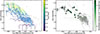 |
Fig. 9. Left: The 253 single-lined hot subdwarf stars shown in the HRD, overlaid with the full set of evolutionary tracks from Han et al. (2002), colour-coded by increasing core mass as indicated by the colour bar. The interpolation and MCMC procedure used to estimate theoretical stellar masses and ages is described in Sect. 7.1. Faded points lie outside the interpolated region and are therefore excluded from mass determination. Right: Same as in the left panel but displaying only the 0.40 and 0.50 M⊙ tracks from Han et al. (2002), and the 183 stars that fit to them. The colour scale shows our expected birthrate calculations as outlined in Sect. 7.5. |
To derive the birthrate, we require a space density, ρ0, and estimated lifetime, τ, of each object. In Paper I we modelled the vertical distribution of the full 500 pc sample and derived the scale height and mid-plane density of the population using a single-component sech2 density profile (see Paper I for details). Here we leverage our kinematic results and employ a three-component sech2 density profile, representing the thin disk, thick disk, and halo populations. Due to low number statistics, we do not fit the scale heights of each component and instead adopt the following: zh, thin = 300 pc, zh, thick = 900 pc, and zh, halo = 2000 pc, which is in line with previous determinations using large samples of stars (see Jurić et al. 2008). The relative contribution of each component is set by the fractional number of stars in our sample identified as belonging to each population (see Table 6):
![Mathematical equation: $$ \begin{aligned} \rho (z) = \frac{1}{N} \bigg [&\rho _{0,\mathrm{thin} } \, \mathrm{sech} ^2\left(\frac{z}{2 z_{h,\mathrm{thin} }}\right) + \rho _{0,\mathrm{thick} } \, \mathrm{sech} ^2\left(\frac{z}{2 z_{h,\mathrm{thick} }}\right) \nonumber \\&+ \rho _{0,\mathrm{halo} } \, \mathrm{sech} ^2\left(\frac{z}{2 z_{h,\mathrm{halo} }}\right) \bigg ]. \end{aligned} $$](/articles/aa/full_html/2026/03/aa58123-25/aa58123-25-eq62.gif) (6)
(6)
Equation (6) gives the normalised stellar number density as a function of vertical height z above the Galactic plane. We then scale the profile vertically by fixing the function to the mid-plane density derived in Paper I: ρ0 = 5.17 ± 0.33 × 10⁻⁷ stars pc−3, thereby ensuring that the profile reflects an absolute space density. Equation (6) therefore represents the expected stellar density (in units of stars/pc3) at position z, and can be used to assign an expected space density for each star based on its position z.
For each star i, we determine the age of the best-fit track at the point of core helium exhaustion, τEHB, i, which defines the transition from the EHB to the post-EHB phase. From this, we can separate the lifetimes of the two stages: the EHB lifetime is τEHB, i, and the post-EHB lifetime is the remaining time, τpEHB, i = τi − τEHB, i, with τi denoting the total lifetime.
Having estimated both the local space density and evolutionary lifetime for each object, we divide the expected space density ρi by the corresponding phase lifetime (τEHB, i or τpEHB, i) obtained from the tracks. This yields an expected birthrate for each of the 183 objects in this experiment, based on their Galactic z-position (through the model-predicted local density) and evolutionary phase. Although not a direct physical birthrate, this quantity traces the relative contribution of stars with different ages and vertical positions to the overall population.
The total estimated birthrates for the EHB and post-EHB stars are derived as
-
 stars/pc3/yr−1 and
 -
 stars/pc3/yr−1.
This may be interpreted as the birthrate of the post-EHB objects being 2–3 times larger than the EHB objects. There could be several reasons for this discrepancy. One possibility is that the post-EHB region includes H-rich stars that are not actually in the post-EHB phase, such as more massive sdBs originating from intermediate-mass progenitors, whose core-helium burning occurs at luminosities above the 0.5 M⊙ EHB, though their lifetimes would be short. Three sdB stars were removed due to high RUWE values (Sect. 6.5), and several stars lie higher up on the EHB beyond the tracks (grey circles), but alone they are not sufficient to explain the 2–3 fold discrepancy because if on the EHB they would count less towards the birthrate than post-EHB objects would due to their longer phase lifetimes. Another possibility is that the EHB lifetimes predicted by the evolutionary tracks of Han et al. (2002) are systematically overestimated, which would directly affect the relative birthrate ratio of EHB to post-EHB stars derived above. Compared with other models, the Han et al. (2002) tracks begin with a higher central helium mass fraction, averaging about 0.973 between the 0.40 and 0.50 M⊙ sequences, which corresponds to an EHB lifetime of about 180 Myr. For comparison, the 0.475 M⊙ solar metallicity models from Dorman et al. (1993) start with a lower central helium fraction of 0.95, yielding a shorter EHB lifetime of ∼136 Myr. However, this modest 1–2% reduction in the available helium fuel would account for only a few Myr difference in the evolutionary timescales of the Han et al. (2002) models. Thus, the substantially longer lifetimes are more plausibly attributed to intrinsic differences in the model physics rather than variations in the initial helium content. Another possible source of inconsistency in the estimated occurrence rates of EHB and post-EHB stars is that our assumed mass range of 0.40 to 0.50 M⊙ may be too narrow, which is likely (see Sect. 6.4).
In addition, some low-mass post-EHB stars at log L/L⊙ > 1.05 may currently be misclassified as EHB stars, which would also exacerbate the discrepancy. More massive EHB stars could also contribute to the post-EHB region, but this is unlikely, as our parallax-based masses exclude values above 0.7 M⊙ at 68% confidence in the range between the 0.40 and 0.50 M⊙ tracks (Fig. 4).
Finally, helium-core white dwarfs evolving towards the cooling sequence are predicted to occupy the same region of parameter space as analysed here (Driebe et al. 1999; Istrate et al. 2016; Althaus et al. 2025), which may also contribute to the observed birthrate discrepancy. Indeed, we identify CPD-20 1123 as a likely candidate, along with the previously known EVR-CB-001. A more detailed investigation of helium-core white dwarfs within this region of parameter space will be presented in a forthcoming paper.
8. Conclusions and outlook
This work extends the spectroscopic study of the 500 pc sample of single-lined hot subdwarf stars introduced in Paper I, providing for the first time a homogeneous analysis of a volume-complete sample. We analysed 3226 spectra of 253 objects by fitting model atmospheres to derive Teff, log g, log n(He)/n(H), and vrad for each star. We further used a subset of our spectra to assess systematic uncertainties in the derived atmospheric parameters. These uncertainties, modelled with third-order polynomial fits, can be added in quadrature to future statistical errors. Stellar masses, radii, and luminosities were determined by combining spectroscopic parameters with SED fits and Gaia parallaxes. The resulting mass distributions and HR diagrams were quantitatively compared with theoretical evolutionary tracks. Finally, using the measured vrad and inferred systemic velocities, we performed a kinematical analysis to determine the Galactic population membership of each object. Our analysis allowed us to draw several conclusions:
-
A significant portion of the observed sample (10 ± 2%; binomial uncertainty) likely originates from intermediate-mass progenitors (1.8 − 8 M⊙), as evidenced by the prominent population of hot subdwarfs situated below the EHB in both the Hertzsprung-Russell and Kiel diagrams. These systems also have, on average, lower masses compared to the general population which is corroborated by theoretical models. This points to a potentially greater contribution from the non-degenerate, no-helium flash formation channel within the Galactic disk than has traditionally been assumed, and encourages future studies in the intermediate-mass regime. A consequence of the significant contribution of low-mass EHB stars implies that assuming canonical masses for hot subdwarfs in single-lined binaries is not reliably justified.
-
We identify two groups of sdBs with extremely helium poor atmospheres (log n(He)/n(H) ≤ −3.8) in the temperature range of 20 000 to 40 000 K. The cool sdBs (Teff < 28 000 K) are almost exclusively located below the EHB, whereas the hotter group (Teff > 34 000 K) is positioned above it, establishing a possible evolutionary link between the cool helium-poor sdBs and the sdO stars. On average, these stars have lower masses (0.41 M⊙) and therefore longer lifetimes. This may allow diffusive effects in the atmospheres in these stars to operate for extended periods, or mixing processes to weaken, leading to lower helium abundances at the stellar surface.
-
Our kinematic analysis, based on astrometry from Gaia and the radial velocities from 3226 spectra of 253 hot subdwarfs, shows that 86 ± 2% belong to the Galactic thin disk, while 13 ± 1% and 1 ± 1% belong to the thick disk and halo populations, respectively. This analysis further revealed that the hot subdwarf stars situated below the EHB are exclusive to the thin disk, which is again consistent with their proposed origin from young intermediate-mass stars.
-
We compared our masses, derived from SED fits using Gaia parallaxes, to theoretical masses calculated by interpolating within the evolutionary tracks from Han et al. (2002) using an MCMC procedure, which returned a strong agreement between them. The HRD-based mass distributions are also narrower than those derived from the Gaia parallax in the SED fits likely owing to the precise luminosities. However, both methods carry significant uncertainties: HRD fitting is affected by degeneracies from overlapping tracks and the choice of models, while parallax-based masses are sensitive to uncertainties in spectroscopic log g measurements.
-
By assuming a restricted mass range for our stars (0.40–0.50 M⊙) and interpolating the corresponding tracks only, we find that the post-EHB birthrate would be 2–3 times higher than the EHB birthrate when adopting a Galactic profile space density for our population based on the results from paper I. A possible reason for the discrepancy is an overestimation of the EHB lifetimes in the tracks of Han et al. (2002). However, other sources of bias and contamination such as the inclusion of H-rich stars in the post-EHB region, which are actually in the EHB phase, cannot be ruled out at this stage.
We provide atmospheric, stellar, and kinematic properties of hot subdwarfs using the first volume-complete sample designed to minimise observational biases. This offers valuable constraints for the next generation of binary population synthesis models. Building on this foundation, forthcoming studies (Dawson et al., in prep.) will present a detailed characterisation of the close binary population within 500 pc, while the 48 wide systems with identified A/F/G-type companions from Paper I will be analysed separately. Just 4 stars within 500 pc are classified as halo objects (Sect. 5), three of them being helium-enriched and the forth a BHB. Therefore, looking ahead, the next major step is to extend volume-complete samples to different galactic environments to incorporate more thick disk and halo stars where we expect to find, for example, a larger fraction of post-merger objects. A new survey targeting the Galactic north pole is nearing completion and will enable a direct comparison of population properties across galactic components in an unbiased way for the first time, providing fresh insight into the role of environment in hot subdwarf formation and evolution.
Data availability
The full versions of Tables 2, 3, and 4 are available at the CDS via https://cdsarc.cds.unistra.fr/viz-bin/cat/J/A+A/707/A6
Acknowledgments
We thank Philipp Podsiadlowski for useful discussions. H. D. was supported by the Deutsche Forschungsgemeinschaft (DFG) through grants GE2506/17-1 and GE2506/9-2. N. R. was supported by the Deutsche Forschungsgemeinschaft (DFG) through grant GE2506/17-1. M. D. was supported by the Deutsches Zentrum für Luft- und Raumfahrt (DLR) through grant 50-OR-2304. V. S. and M. P. received funding by the Deutsche Forschungsgemeinschaft (DFG) through grants GE2506/9-1 and GE2506/12-1. D. S. acknowledges funding by DFG grant HE1356/70-1. I. P. acknowledges funding from a Warwick Astrophysics prize post-doctoral fellowship, made possible thanks to a generous philanthropic donation, and from a Royal Society University Research Fellowship (URF\R1\231496). J. V. acknowledges support from the Grant Agency of the Czech Republic (GAČR 22-34467S). The Astronomical Institute Ondřejov is supported by the project RVO:67985815. M. U. gratefully acknowledges funding from the Research Foundation Flanders (FWO) by means of a junior postdoctoral fellowship (grant agreement No. 1247624N). K. D. acknowledges funding from the Methusalem grant METH/24/012 at KU Leuven. This research has used observations obtained at the Mercator Observatory which receives funding from the Research Foundation – Flanders (FWO) (grant agreement I000325N and I000521N). A. B. was supported by the Deutsche Forschungsgemeinschaft (DFG) through grant GE2506/18-1. T. S. acknowledges funding from grant SONATA BIS no 2018/30/E/ST9/00398 from the Polish National Science Centre (PI T. Kamiński). R. R. acknowledges support from Grant RYC2021-030837-I funded by MCIN/AEI/ 10.13039/501100011033 and by “European Union NextGeneration EU/PRTR”. This work was partially supported by Spanish MINECO grant PID2023-148661NB-I00. T. K. acknowledges support from the National Science Foundation through grant AST #2107982, from NASA through grant 80NSSC22K0338 and from STScI through grant HST-GO-16659.002-A. Co-funded by the European Union (ERC, CompactBINARIES, 101078773). Views and opinions expressed are however those of the author(s) only and do not necessarily reflect those of the European Union or the European Research Council. Neither the European Union nor the granting authority can be held responsible for them. M. L. acknowledges funding from the DFG (grant LA 4383/4-1). M. V. acknowledges support from the FONDECYT Regular N° 1211941 and N° 1250525. This project has received funding from the European Research Council under the European Union’s Horizon 2020 research and innovation programme (Grant agreement numbers 101002408). Based on observations collected with the Goodman spectrograph at the Southern Astrophysical Research Facility (SOAR) at Cerro Pachon, Chile, under the programme allocated by the Chilean Telescope Allocation Committee (CNTAC), no: 2023B, 2024A and 2025A. This work has made use of the BeSS database, operated at LESIA, Observatoire de Meudon, France: http://basebe.obspm.fr. Some data in this worked came from Guaranteed Observation Time (GTO) based on observations collected at the Centro Astronomico Hispano en Andalucia (CAHA) at Calar Alto, operated jointly by Junta de Andalucia and Cosejo Superior De Investigaciones Cientificias (IAA-CSIC). The research has made use of TOPCAT, an interactive graphical viewer and editor for tabular data (Taylor 2005). This research made use of the SIMBAD database, operated at CDS, Strasbourg, France; the VizieR catalogue access tool, CDS, Strasbourg, France. This work has made use of data from the European Space Agency (ESA) mission Gaia (https://www.cosmos.esa.int/gaia), processed by the Gaia Data Processing and Analysis Consortium (DPAC, https://www.cosmos.esa.int/web/gaia/dpac/consortium). Funding for the DPAC has been provided by national institutions, in particular the institutions participating in the Gaia Multilateral Agreement.
References
- Akima, H. 1970, J. ACM, 17, 589 [Google Scholar]
- Althaus, L. G., Calcaferro, L. M., Córsico, A. H., & Brown, W. R. 2025, A&A, 699, A280 [NASA ADS] [CrossRef] [EDP Sciences] [Google Scholar]
- Anguiano, B., Majewski, S. R., Hayes, C. R., et al. 2020, AJ, 160, 43 [NASA ADS] [CrossRef] [Google Scholar]
- Arancibia-Rojas, E., Zorotovic, M., Vučković, M., et al. 2024, MNRAS, 527, 11184 [Google Scholar]
- Battich, T., Miller Bertolami, M. M., Córsico, A. H., & Althaus, L. G. 2018, A&A, 614, A136 [NASA ADS] [CrossRef] [EDP Sciences] [Google Scholar]
- Bilir, S., Karaali, S., Ak, S., Yaz, E., & Hamzaoğlu, E. 2006, New Astron., 12, 234 [Google Scholar]
- Bland-Hawthorn, J., & Gerhard, O. 2016, ARA&A, 54, 529 [Google Scholar]
- Bovy, J., Hogg, D. W., & Roweis, S. T. 2011, Ann. Appl. Stat., 5, 1657 [Google Scholar]
- Brown, T. M., Sweigart, A. V., Lanz, T., Landsman, W. B., & Hubeny, I. 2001, ApJ, 562, 368 [NASA ADS] [CrossRef] [Google Scholar]
- Byrne, C. M., Jeffery, C. S., Tout, C. A., & Hu, H. 2018, MNRAS, 475, 4728 [NASA ADS] [CrossRef] [Google Scholar]
- Canbay, R., Bilir, S., Özdönmez, A., & Ak, T. 2023, AJ, 165, 163 [NASA ADS] [CrossRef] [Google Scholar]
- Cassisi, S., Salaris, M., & Pietrinferni, A. 2016, Mem. Soc. Astron. It., 87, 332 [NASA ADS] [Google Scholar]
- Castellani, M., & Castellani, V. 1993, ApJ, 407, 649 [NASA ADS] [CrossRef] [Google Scholar]
- Clausen, D., Wade, R. A., Kopparapu, R. K., & O’Shaughnessy, R. 2012, ApJ, 746, 186 [NASA ADS] [CrossRef] [Google Scholar]
- Copperwheat, C. M., Morales-Rueda, L., Marsh, T. R., Maxted, P. F. L., & Heber, U. 2011, MNRAS, 415, 1381 [Google Scholar]
- Cox, J. P., & Salpeter, E. E. 1964, ApJ, 140, 485 [Google Scholar]
- Culpan, R., Pelisoli, I., & Geier, S. 2021, VizieR Online Data Catalog, J/A+A/654/A107 [Google Scholar]
- Culpan, R., Geier, S., Reindl, N., et al. 2022, A&A, 662, A40 [NASA ADS] [CrossRef] [EDP Sciences] [Google Scholar]
- Culpan, R., Dorsch, M., Geier, S., et al. 2024, A&A, 685, A134 [NASA ADS] [CrossRef] [EDP Sciences] [Google Scholar]
- Dawson, H., Geier, S., Heber, U., et al. 2024, A&A, 686, A25 [NASA ADS] [CrossRef] [EDP Sciences] [Google Scholar]
- Dempster, A. P., Laird, N. M., & Rubin, D. B. 1977, J. R. Stat. Soc. B, 39, 1 [Google Scholar]
- Derekas, A., Németh, P., Southworth, J., et al. 2015, ApJ, 808, 179 [NASA ADS] [CrossRef] [Google Scholar]
- DESI Collaboration (Abdul-Karim, M., et al.) 2025, arXiv e-prints [arXiv:2503.14745] [Google Scholar]
- Dorman, B., Rood, R. T., & O’Connell, R. W. 1993, ApJ, 419, 596 [NASA ADS] [CrossRef] [Google Scholar]
- Dorsch, M. 2024, Ph.D. Thesis, Friedrich Alexander University of Erlangen-Nuremberg, Germany [Google Scholar]
- Driebe, T., Schönberner, D., Blöcker, T., & Herwig, F. 1999, ASP Conf. Ser., 169, 394 [Google Scholar]
- Edelmann, H., Heber, U., Hagen, H. J., et al. 2003, A&A, 400, 939 [NASA ADS] [CrossRef] [EDP Sciences] [Google Scholar]
- El-Badry, K., Rix, H.-W., & Heintz, T. M. 2021, MNRAS, 506, 2269 [NASA ADS] [CrossRef] [Google Scholar]
- Fitzpatrick, E. L., Massa, D., Gordon, K. D., Bohlin, R., & Clayton, G. C. 2019, ApJ, 886, 108 [Google Scholar]
- Fontaine, G., & Chayer, P. 1997, in The Third Conference on Faint Blue Stars, eds. A. G. D. Philip, J. Liebert, R. Saffer, & D. S. Hayes, 169 [Google Scholar]
- Fontaine, G., Brassard, P., Charpinet, S., et al. 2012, A&A, 539, A12 [NASA ADS] [CrossRef] [EDP Sciences] [Google Scholar]
- Fontaine, G., Green, E., Brassard, P., Latour, M., & Chayer, P. 2014, ASP Conf. Ser., 481, 83 [Google Scholar]
- Gaia Collaboration. 2020, VizieR Online Data Catalog, I/350 [Google Scholar]
- Gaia Collaboration (Vallenari, A., et al.) 2023, A&A, 674, A1 [NASA ADS] [CrossRef] [EDP Sciences] [Google Scholar]
- Geier, S. 2013, A&A, 549, A110 [NASA ADS] [CrossRef] [EDP Sciences] [Google Scholar]
- Geier, S. 2020, A&A, 635, A193 [NASA ADS] [CrossRef] [EDP Sciences] [Google Scholar]
- Geier, S., & Heber, U. 2012, A&A, 543, A149 [NASA ADS] [CrossRef] [EDP Sciences] [Google Scholar]
- Geier, S., Edelmann, H., Heber, U., & Morales-Rueda, L. 2009, ApJ, 702, L96 [Google Scholar]
- Geier, S., Østensen, R. H., Nemeth, P., et al. 2017, A&A, 600, A50 [NASA ADS] [CrossRef] [EDP Sciences] [Google Scholar]
- Geier, S., Dorsch, M., Pelisoli, I., et al. 2022, A&A, 661, A113 [NASA ADS] [CrossRef] [EDP Sciences] [Google Scholar]
- Geier, S., Heber, U., Irrgang, A., et al. 2024, A&A, 690, A368 [NASA ADS] [CrossRef] [EDP Sciences] [Google Scholar]
- Giddings, J. R. 1980, Ph.D. Thesis, University College London, UK [Google Scholar]
- Gilmore, G., & Reid, N. 1983, MNRAS, 202, 1025 [Google Scholar]
- Götberg, Y., de Mink, S. E., Groh, J. H., et al. 2018, A&A, 615, A78 [NASA ADS] [CrossRef] [EDP Sciences] [Google Scholar]
- Gould, N. L., Herbig, G. H., & Morgan, W. W. 1957, PASP, 69, 242 [Google Scholar]
- Greenstein, J. L., & Sargent, A. I. 1974, ApJS, 28, 157 [Google Scholar]
- Han, Z. 2008, A&A, 484, L31 [NASA ADS] [CrossRef] [EDP Sciences] [Google Scholar]
- Han, Z., Podsiadlowski, P., Maxted, P. F. L., Marsh, T. R., & Ivanova, N. 2002, MNRAS, 336, 449 [Google Scholar]
- Han, Z., Podsiadlowski, P., Maxted, P. F. L., & Marsh, T. R. 2003, MNRAS, 341, 669 [NASA ADS] [CrossRef] [Google Scholar]
- Hansen, C. J., & Spangenberg, W. 1971, ApJ, 163, 653 [Google Scholar]
- He, R., Meng, X., Lei, Z., Yan, H., & Lan, S. 2025, A&A, 693, A121 [NASA ADS] [CrossRef] [EDP Sciences] [Google Scholar]
- Heber, U. 2009, ARA&A, 47, 211 [Google Scholar]
- Heber, U. 2016, PASP, 128, 082001 [Google Scholar]
- Heber, U. 2026, Encycl. Astrophys., 2, 488 [Google Scholar]
- Heber, U., Hunger, K., Jonas, G., & Kudritzki, R. P. 1984, A&A, 130, 119 [NASA ADS] [Google Scholar]
- Heber, U., Reid, I. N., & Werner, K. 2000, A&A, 363, 198 [NASA ADS] [Google Scholar]
- Heber, U., Edelmann, H., Lisker, T., & Napiwotzki, R. 2003, A&A, 411, L477 [NASA ADS] [CrossRef] [EDP Sciences] [Google Scholar]
- Heber, U., Irrgang, A., & Schaffenroth, J. 2018, Open Astron., 27, 35 [Google Scholar]
- Heber, U., Kufleitner, L., Dorsch, M., et al. 2025, A&A, submitted [Google Scholar]
- Hogg, D. W., Bovy, J., & Lang, D. 2010, ArXiv e-prints [arXiv:1008.4686] [Google Scholar]
- Houck, J. C., & Denicola, L. A. 2000, ASP Conf. Ser., 216, 591 [Google Scholar]
- Hu, H., Dupret, M. A., Aerts, C., et al. 2008, A&A, 490, 243 [NASA ADS] [CrossRef] [EDP Sciences] [Google Scholar]
- Hu, H., Tout, C. A., Glebbeek, E., & Dupret, M. A. 2011, MNRAS, 418, 195 [NASA ADS] [CrossRef] [Google Scholar]
- Husser, T. O., Wende-von Berg, S., Dreizler, S., et al. 2013, A&A, 553, A6 [NASA ADS] [CrossRef] [EDP Sciences] [Google Scholar]
- Irrgang, A. 2014, Ph.D. Thesis, Friedrich-Alexander-Universität Erlangen-Nürnberg [Google Scholar]
- Irrgang, A., Wilcox, B., Tucker, E., & Schiefelbein, L. 2013, A&A, 549, A137 [NASA ADS] [CrossRef] [EDP Sciences] [Google Scholar]
- Irrgang, A., Kreuzer, S., Heber, U., & Brown, W. 2018, A&A, 615, L5 [NASA ADS] [CrossRef] [EDP Sciences] [Google Scholar]
- Istrate, A. G., Marchant, P., Tauris, T. M., et al. 2016, A&A, 595, A35 [NASA ADS] [CrossRef] [EDP Sciences] [Google Scholar]
- Jacobs, V. A., Østensen, R. H., van Winckel, H., et al. 2011, AIP Conf. Ser., 1331, 304 [Google Scholar]
- Jeffery, C. S., & Ramsay, G. 2014, MNRAS, 442, L61 [NASA ADS] [CrossRef] [Google Scholar]
- Jeffery, C. S., & Zhang, X. 2020, JApA, 41, 48 [NASA ADS] [Google Scholar]
- Johnson, D. R. H., & Soderblom, D. R. 1987, AJ, 93, 864 [Google Scholar]
- Jurić, M., Ivezić, Ž., Brooks, A., et al. 2008, ApJ, 673, 864 [Google Scholar]
- Justham, S., Podsiadlowski, P., & Han, Z. 2011, MNRAS, 410, 984 [CrossRef] [Google Scholar]
- Kawka, A., Vennes, S., O’Toole, S., et al. 2015, MNRAS, 450, 3514 [Google Scholar]
- Kelly, B. C. 2007, ApJ, 665, 1489 [Google Scholar]
- Kepler, S. O., Pelisoli, I., Koester, D., et al. 2019, MNRAS, 486, 2169 [NASA ADS] [Google Scholar]
- Khalack, V., Yameogo, B., LeBlanc, F., et al. 2014, MNRAS, 445, 4086 [NASA ADS] [CrossRef] [Google Scholar]
- Krzesinski, J.& Balona, L. A. 2022, VizieR On-line Data Catalog: J/A+A/663/A45 [Google Scholar]
- Kupfer, T., Geier, S., Heber, U., et al. 2015, A&A, 576, A44 [NASA ADS] [CrossRef] [EDP Sciences] [Google Scholar]
- Kurucz, R. L. 1996, ASP Conf. Ser., 108, 160 [NASA ADS] [Google Scholar]
- Lanz, T., Brown, T. M., Sweigart, A. V., Hubeny, I., & Landsman, W. B. 2004, ApJ, 602, 342 [CrossRef] [Google Scholar]
- Latour, M., Randall, S. K., Fontaine, G., et al. 2014, ApJ, 795, 106 [NASA ADS] [CrossRef] [Google Scholar]
- Latour, M., Heber, U., Irrgang, A., et al. 2016, A&A, 585, A115 [NASA ADS] [CrossRef] [EDP Sciences] [Google Scholar]
- Latour, M., Chayer, P., Green, E. M., Irrgang, A., & Fontaine, G. 2018a, A&A, 609, A89 [NASA ADS] [CrossRef] [EDP Sciences] [Google Scholar]
- Latour, M., Randall, S. K., Calamida, A., Geier, S., & Moehler, S. 2018b, A&A, 618, A15 [NASA ADS] [CrossRef] [EDP Sciences] [Google Scholar]
- Latour, M., Green, E. M., & Fontaine, G. 2019, A&A, 623, L12 [NASA ADS] [CrossRef] [EDP Sciences] [Google Scholar]
- Latour, M., Green, E. M., Dorsch, M., et al. 2026, A&A, 705, A248 [Google Scholar]
- Lei, Z., Zhao, J., Németh, P., & Zhao, G. 2018, ApJ, 868, 70 [Google Scholar]
- Lei, Z., Zhao, J., Németh, P., & Zhao, G. 2019, ApJ, 881, 135 [NASA ADS] [CrossRef] [Google Scholar]
- Lei, Z., Zhao, J., Németh, P., & Zhao, G. 2020, ApJ, 889, 117 [NASA ADS] [CrossRef] [Google Scholar]
- Lei, Z., He, R., Németh, P., et al. 2023a, ApJ, 942, 109 [CrossRef] [Google Scholar]
- Lei, Z., He, R., Németh, P., et al. 2023b, ApJ, 953, 122 [NASA ADS] [CrossRef] [Google Scholar]
- Luo, Y.-P., Németh, P., Liu, C., Deng, L.-C., & Han, Z.-W. 2016, ApJ, 818, 202 [NASA ADS] [CrossRef] [Google Scholar]
- Luo, Y., Németh, P., Deng, L., & Han, Z. 2019, ApJ, 881, 7 [NASA ADS] [CrossRef] [Google Scholar]
- Luo, Y., Németh, P., Wang, K., Wang, X., & Han, Z. 2021, ApJS, 256, 28 [NASA ADS] [CrossRef] [Google Scholar]
- Luo, A. L., Zhao, Y. H., Zhao, G., et al. 2022, VizieR Online Data Catalog, V/156 [Google Scholar]
- Ma, X., Hopkins, P. F., Wetzel, A. R., et al. 2017, MNRAS, 467, 2430 [Google Scholar]
- Marsh, T. R. 1989, PASP, 101, 1032 [Google Scholar]
- Marsh, T. 2019, Astrophysics Source Code Library [record ascl:1907.012] [Google Scholar]
- Maxted, P. F. L., Heber, U., Marsh, T. R., & North, R. C. 2001, MNRAS, 326, 1391 [CrossRef] [Google Scholar]
- McLachlan, G. J., & Peel, D. 2000, Finite Mixture Models, illustrated edn. (John Wiley& Sons), Wiley Ser. Probab. Stat., 464 [Google Scholar]
- Michaud, G., Richer, J., & Richard, O. 2011, A&A, 529, A60 [NASA ADS] [CrossRef] [EDP Sciences] [Google Scholar]
- Miller Bertolami, M. M., Althaus, L. G., Unglaub, K., & Weiss, A. 2008, A&A, 491, 253 [NASA ADS] [CrossRef] [EDP Sciences] [Google Scholar]
- Moehler, S., Richtler, T., de Boer, K. S., Dettmar, R. J., & Heber, U. 1990, A&AS, 86, 53 [Google Scholar]
- Morales-Rueda, L., Maxted, P. F. L., Marsh, T. R., North, R. C., & Heber, U. 2003, MNRAS, 338, 752 [CrossRef] [Google Scholar]
- Moran, C., Maxted, P., Marsh, T. R., Saffer, R. A., & Livio, M. 1999, MNRAS, 304, 535 [NASA ADS] [CrossRef] [Google Scholar]
- Napiwotzki, R., Karl, C. A., Lisker, T., et al. 2004, Ap&SS, 291, 321 [NASA ADS] [CrossRef] [Google Scholar]
- Naslim, N., Geier, S., Jeffery, C. S., et al. 2012, MNRAS, 423, 3031 [NASA ADS] [CrossRef] [Google Scholar]
- Németh, P., Kawka, A., & Vennes, S. 2012, MNRAS, 427, 2180 [Google Scholar]
- Newell, E. B. 1973, ApJS, 26, 37 [Google Scholar]
- Ostensen, R., Heber, U., & Maxted, P. 2005, ASP Conf. Ser., 334, 435 [Google Scholar]
- Ostrowski, J., Baran, A. S., Sanjayan, S., & Sahoo, S. K. 2021, MNRAS, 503, 4646 [Google Scholar]
- Paczyński, B. 1971, Acta Astron., 21, 1 [NASA ADS] [Google Scholar]
- Pauli, E. M., Napiwotzki, R., Heber, U., Altmann, M., & Odenkirchen, M. 2006, A&A, 447, 173 [NASA ADS] [CrossRef] [EDP Sciences] [Google Scholar]
- Pelisoli, I., Vos, J., Geier, S., Schaffenroth, V., & Baran, A. S. 2020, A&A, 642, A180 [NASA ADS] [CrossRef] [EDP Sciences] [Google Scholar]
- Pereira, C. 2011, Ph.D. Thesis, Queens University Belfast, Ireland [Google Scholar]
- Prada Moroni, P. G., & Straniero, O. 2009, J. Phys. Conf. Ser., 172, 012011 [Google Scholar]
- Ramspeck, M., Heber, U., & Edelmann, H. 2001, A&A, 379, 235 [NASA ADS] [CrossRef] [EDP Sciences] [Google Scholar]
- Randall, S. K., Bagnulo, S., Ziegerer, E., Geier, S., & Fontaine, G. 2015, A&A, 576, A65 [NASA ADS] [CrossRef] [EDP Sciences] [Google Scholar]
- Raskin, G., van Winckel, H., Hensberge, H., et al. 2011, A&A, 526, A69 [CrossRef] [EDP Sciences] [Google Scholar]
- Ratzloff, J. K., Barlow, B. N., Kupfer, T., et al. 2019, ApJ, 883, 51 [NASA ADS] [CrossRef] [Google Scholar]
- Reindl, N., Rauch, T., Werner, K., Kruk, J. W., & Todt, H. 2014, A&A, 566, A116 [NASA ADS] [CrossRef] [EDP Sciences] [Google Scholar]
- Reindl, N., Geier, S., Kupfer, T., et al. 2016, A&A, 587, A101 [NASA ADS] [CrossRef] [EDP Sciences] [Google Scholar]
- Reindl, N., Bond, H. E., Werner, K., & Zeimann, G. R. 2024, A&A, 690, A366 [NASA ADS] [CrossRef] [EDP Sciences] [Google Scholar]
- Rodríguez-Segovia, N. 2025, Ph.D. Thesis, UNSW, Sydney [Google Scholar]
- Rodríguez-Segovia, N., & Ruiter, A. J. 2025, MNRAS, 539, 3273 [Google Scholar]
- Rodríguez-Segovia, N., Ruiter, A. J., & Seitenzahl, I. R. 2025, PASA, 42, e012 [Google Scholar]
- Saffer, R. A., Livio, M., & Yungelson, L. R. 1998, ApJ, 502, 394 [Google Scholar]
- Saio, H., & Jeffery, C. S. 2000, MNRAS, 313, 671 [NASA ADS] [CrossRef] [Google Scholar]
- Schaffenroth, V., Pelisoli, I., Barlow, B. N., Geier, S., & Kupfer, T. 2022, A&A, 666, A182 [NASA ADS] [CrossRef] [EDP Sciences] [Google Scholar]
- Schaffenroth, V., Barlow, B. N., Pelisoli, I., Geier, S., & Kupfer, T. 2023, A&A, 673, A90 [NASA ADS] [CrossRef] [EDP Sciences] [Google Scholar]
- Schindewolf, M. 2018, Ph.D. Thesis, Friedrich-Alexander-Universität Erlangen-Nürnberg [Google Scholar]
- Schneider, D., Irrgang, A., Heber, U., Nieva, M. F., & Przybilla, N. 2018, A&A, 618, A86 [NASA ADS] [CrossRef] [EDP Sciences] [Google Scholar]
- Schönrich, R., Binney, J., & Dehnen, W. 2010, MNRAS, 403, 1829 [NASA ADS] [CrossRef] [Google Scholar]
- Science Software Branch at STScI. 2012, Astrophysics Source Code Library [record ascl:1207.011] [Google Scholar]
- Şener, H. T., & Jeffery, C. S. 2014, MNRAS, 440, 2676 [NASA ADS] [CrossRef] [Google Scholar]
- Stroeer, A., Heber, U., Lisker, T., et al. 2007, A&A, 462, 269 [NASA ADS] [CrossRef] [EDP Sciences] [Google Scholar]
- Sweigart, A. V. 1997, ApJ, 474, L23 [NASA ADS] [CrossRef] [Google Scholar]
- Sweigart, A. V., & Gross, P. G. 1978, ApJS, 36, 405 [NASA ADS] [CrossRef] [Google Scholar]
- Taylor, M. B. 2005, ASP Conf. Ser., 347, 29 [Google Scholar]
- Tody, D. 1986, SPIE Conf. Ser., 627, 733 [Google Scholar]
- Unglaub, K. 2008, A&A, 486, 923 [NASA ADS] [CrossRef] [EDP Sciences] [Google Scholar]
- Vennes, S., Kawka, A., & Smith, J. A. 2007, ApJ, 668, L59 [Google Scholar]
- Villeneuve, B., Wesemael, F., & Fontaine, G. 1995a, ApJ, 450, 851 [NASA ADS] [CrossRef] [Google Scholar]
- Villeneuve, B., Wesemael, F., Fontaine, G., Carignan, C., & Green, R. F. 1995b, ApJ, 446, 646 [NASA ADS] [CrossRef] [Google Scholar]
- Vos, J., Bobrick, A., & Vučković, M. 2020, A&A, 641, A163 [NASA ADS] [CrossRef] [EDP Sciences] [Google Scholar]
- Webbink, R. F. 1984, ApJ, 277, 355 [NASA ADS] [CrossRef] [Google Scholar]
- Widrow, L. M., Gardner, S., Yanny, B., Dodelson, S., & Chen, H.-Y. 2012, ApJ, 750, L41 [Google Scholar]
- Xiong, H., Chen, X., Podsiadlowski, P., Li, Y., & Han, Z. 2017, A&A, 599, A54 [NASA ADS] [CrossRef] [EDP Sciences] [Google Scholar]
- Yoachim, P., & Dalcanton, J. J. 2006, AJ, 131, 226 [NASA ADS] [CrossRef] [Google Scholar]
- Yungelson, L. R. 2008, Astron. Lett., 34, 620 [Google Scholar]
- Zhang, X., & Jeffery, C. S. 2012, MNRAS, 419, 452 [NASA ADS] [CrossRef] [Google Scholar]
A detailed study of the binary population will be given in a follow-up paper.
The covariance matrix between log Teff and log L was estimated from a sample of 50 000 Monte Carlo draws from the SED fitting posteriors. This accounts for observational uncertainties and correlations between parameters during the MCMC sampling.
See their Fig. 4 for an illustration of the relation between He-core masses and the masses of the progenitor stars on the main sequence.
Appendix A: Additional tables and figures
Included hot subdwarfs with a hint of IR excess.
Coefficients of the third-order polynomial fits to the systematic uncertainty for each parameter as in Eq. 1. The coefficients for Teff are given in kilokelvin.
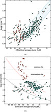 |
Fig. A.1. log g versus effective temperature (top) and helium abundance versus effective temperature (bottom) showing the impact of metallicity in these parameter spaces. Circles and squares mark the helium-poor (log n(He)/n(H) < –1.2) and helium-rich (log n(He)/n(H) > –1.2) stars, respectively, for fits fixed to a metallicity of log z/zsdB = 0. Grey and bronze triangles, oriented such that they point down and up, respectively, show the parameters derived for these same stars when fixing the metallicity to log z/zsdB = − 0.3 and +0.3, respectively. Each triangle is connected by a black line to the circle or square to indicate the shift. |
All Tables
Coefficients of the third-order polynomial fits to the systematic uncertainty for each parameter as in Eq. 1. The coefficients for Teff are given in kilokelvin.
All Figures
|
Fig. 1. Example spectral fits (red) to various hot subdwarfs (black) using the pipeline described in Sect. 4. Table 1 provides more details about the spectra. |
| In the text | |
|
Fig. 2. Three-panel figure showing our best estimates of the overall uncertainties in Teff, log g, and log n(He)/n(H) (from left to right), displayed as scattered markers. The Teff uncertainties are plotted as fractional values (ΔTeff/Teff, i.e. 1–5%). Helium-rich and helium-poor stars are separated and indicated as orange squares and dark blue circles, respectively. The solid orange and dark blue lines are polynomial fits (Equation (1)) to these scattered markers, and the coefficients of these are given in Table A.2. The dashed polynomials represent the identified uncertainty contributions from the intrinsic scatter measured in our INT data and from the metallicity abundance uncertainty, as described in Sect. 4.2. The formal statistical errors are given by the error bars of the scattered markers and the instrumental offset between INT and ALFOSC is given by a black-dashed line. All four identified uncertainties are added together in quadrature to arrive at the uncertainties used for the analysis in this work. |
| In the text | |
|
Fig. 3. Upper left: Teff − log g diagram of the hot subdwarf stars in the 500 pc sample, colour-coded as shown in the legend (lower panel). Three post-EHB evolutionary tracks for three different envelope masses from Han et al. (2003) are given as solid-black lines: 0.00, 0.001, and 0.005 M⊙ from bottom to top (Mtotal = 0.45 M⊙). The thickness of the lines are linearly proportional to the predicted evolutionary time. A double He-WD merger track from Zhang & Jeffery (2012) is shown as a orange dot-dashed line. The region encapsulated by the zero-age EHB and the terminal-age EHB from Dorman et al. (1993) is depicted as a shaded light-blue region which extends down to the He-MS from Paczyński (1971) which is shown as a dotted-grey line. All tracks are given for solar metallicity. Upper right: helium abundance – Teff diagram for the same stars. The helium sequences identified in earlier studies (Edelmann et al. 2003; Németh et al. 2012; Luo et al. 2016; Lei et al. 2018) are shown. Bottom: Hertzsprung-Russell diagram with the same hot subdwarf classes and evolutionary tracks as shown in the upper left panel. The He-MS from Paczyński (1971) is again shown as a dotted-grey line with the corresponding masses annotated. The horizontal dashed-black lines indicate the solar metallicity ZAEHB at log L/L⊙ = 1.05 at the start of the 0.45 M⊙ evolutionary tracks from Han et al. (2002), and the TAEHB of these tracks at the point of core helium depletion. Two additional ZAEHB positions are marked as dashed-red lines for the 0.40 M⊙ and 0.35 M⊙ evolutionary tracks to compare with the low-luminosity objects. Black pentagons mark the underluminous hot subdwarfs (log L/L⊙ < 1.05) in all three plots. Crimson pentagons indicate the three identified hot and helium-poor stars. The grey star marks the previous position of HD 188112. |
| In the text | |
|
Fig. 4. Distribution of our stars in the mass – effective temperature plane. The He-MS (Paczyński 1971) is shown as a dashed grey line. The grey-shaded band is centred on a mass of 0.47 M⊙ and spans ±0.05 M⊙, corresponding to our mean uncertainties. The pink-shaded region extends down to 0.35 M⊙, the minimum core mass predicted by the evolutionary tracks of Han et al. (2002). Pentagons indicate the same stars as in Fig. 3. |
| In the text | |
|
Fig. 5. KDE representation of the mass and luminosity distributions for the full sample and subgroups of hot subdwarf stars. Uncertainties are not included in the KDEs, allowing clearer comparison between different hot subdwarf classes. |
| In the text | |
|
Fig. 6. Same KDEs as presented in Fig. 5, but using theoretical masses derived from our MCMC interpolation procedure in the HRD described in Sect. 7.1. Additionally, the right panel shows the estimated mass distributions of the He-rich stars derived by projecting each object to its nearest point along the He-MS (Paczyński 1971) in the HRD. |
| In the text | |
|
Fig. 7. Distribution of the 500 pc sample in the W-V, U-V, W-U, and Toomre (lower right) diagrams. The stars are marked as light blue circles, dark blue squares, and orange triangles to indicate thin disk, thick disk and halo membership, respectively. Two-sigma contours of the Galactic components are given in the same colour scheme. The position of the Sun is given by the black circle. |
| In the text | |
|
Fig. 8. Three-panel plot showing the HRDs for the thin disk, thick disk, and halo populations in our sample, as determined from our kinematic analysis in Sect. 5. The Solar-metallicity ZAEHB at L/L⊙ = 1.05 is overlaid to highlight that only objects associated with the thin disk population fall below the EHB. |
| In the text | |
|
Fig. 9. Left: The 253 single-lined hot subdwarf stars shown in the HRD, overlaid with the full set of evolutionary tracks from Han et al. (2002), colour-coded by increasing core mass as indicated by the colour bar. The interpolation and MCMC procedure used to estimate theoretical stellar masses and ages is described in Sect. 7.1. Faded points lie outside the interpolated region and are therefore excluded from mass determination. Right: Same as in the left panel but displaying only the 0.40 and 0.50 M⊙ tracks from Han et al. (2002), and the 183 stars that fit to them. The colour scale shows our expected birthrate calculations as outlined in Sect. 7.5. |
| In the text | |
|
Fig. A.1. log g versus effective temperature (top) and helium abundance versus effective temperature (bottom) showing the impact of metallicity in these parameter spaces. Circles and squares mark the helium-poor (log n(He)/n(H) < –1.2) and helium-rich (log n(He)/n(H) > –1.2) stars, respectively, for fits fixed to a metallicity of log z/zsdB = 0. Grey and bronze triangles, oriented such that they point down and up, respectively, show the parameters derived for these same stars when fixing the metallicity to log z/zsdB = − 0.3 and +0.3, respectively. Each triangle is connected by a black line to the circle or square to indicate the shift. |
| In the text | |
Current usage metrics show cumulative count of Article Views (full-text article views including HTML views, PDF and ePub downloads, according to the available data) and Abstracts Views on Vision4Press platform.
Data correspond to usage on the plateform after 2015. The current usage metrics is available 48-96 hours after online publication and is updated daily on week days.
Initial download of the metrics may take a while.