| Issue |
A&A
Volume 707, March 2026
|
|
|---|---|---|
| Article Number | A322 | |
| Number of page(s) | 17 | |
| Section | Galactic structure, stellar clusters and populations | |
| DOI | https://doi.org/10.1051/0004-6361/202558153 | |
| Published online | 20 March 2026 | |
Homogeneous abundances of Mg, Si, Ca, and Ti for about 1500 red giants in 16 globular clusters from FLAMES spectra★
INAF - Osservatorio di Astrofisica e Scienza dello Spazio di Bologna,
Via P. Gobetti 93/3,
40129
Bologna,
Italy
★★ Corresponding author: This email address is being protected from spambots. You need JavaScript enabled to view it.
Received:
17
November
2025
Accepted:
23
January
2026
Abstract
The FLAMES survey ‘Na-O anti-correlation and HB’ uncovered the modern standard for globular clusters (GCs), which is their ubiquitous multiple stellar populations (MPs) distinguished by the abundance of proton-capture elements. That survey can still be mined to extract a wealth of data. We derive new abundances of Mg, Si, Ca, and Ti for 948, 954, 1542, and 1350 red giant branch stars in 16 GCs, both formed in situ or accreted in the Milky Way. The programme GCs cover the metallicity range from [Fe∕H]=-2.35 dex to [Fe∕H]=-0.74 dex. Both the halo and disc GCs show a clear overabundance of α-elements with the modulation in Mg and Si due to the MPs phenomenon in different clusters. We found star to star variations in Si abundance correlated to changes in Na in more than half our sample, implying that temperatures in excess of about 65 MK were achieved in the polluters responsible for the enrichment. We confirm with an enlarged sample the previous result that significant variations in Mg are observed in GCs that are metal-poor, massive or both. Evidence of excess of Ca with respect to reference unpolluted field stars are found in NGC 6752 and NGC 7078, indicating the action of proton-capture reactions at very high temperature regime in these GCs. These excesses fit very well in a previously found relation as a function of a combination of cluster mass and metallicity shown by other typical signatures of MPs. At odds with previous results based on the Si abundance from APOGEE, we found that the average abundance of α-elements is not an efficient discriminating factor between in situ and accreted GCs.
Key words: stars: abundances / stars: atmospheres / stars: Population II / globular clusters: general
Based on observations collected at ESO telescopes under programmes 072.D-507 and 073.D-0211.
© The Authors 2026
 Open Access article, published by EDP Sciences, under the terms of the Creative Commons Attribution License (https://creativecommons.org/licenses/by/4.0), which permits unrestricted use, distribution, and reproduction in any medium, provided the original work is properly cited.
This article is published in open access under the Subscribe to Open model. This email address is being protected from spambots. You need JavaScript enabled to view it. to support open access publication.
1 Introduction
Globular clusters (GCs) represent a major component of old stellar populations in galaxies. Being bright, they are accessible even at large distances, providing a useful link between the local population in the Milky Way and external galaxies, including the high-redshift objects presently being studied with new generation space telescopes (e.g. Adamo et al. 2024). For some decades, GCs were considered as the first stellar aggregates to originate in galaxies and were thought to be the best specimen of simple stellar populations (coeval groups of stars with homogeneous initial chemical composition). In relatively recent times, both statements underwent severe revisions. Since the seminal paper by Searle & Zinn (1978) it was recognised that only a part of GCs originated in the main body (bulge or disc) of the protogalaxy, within dissipational collapse as in the scenario devised by Eggen et al. (1962). About half of the GCs population formed in individual fragments, later accreted in the Galaxy. It is well known that the luminosity function of the outer halo GCs is similar to that of GCs in dwarf spheroidal galaxies (e.g. Carretta et al. 2010a).
Second, the pioneering efforts of the Lick-Texas group (Kraft 1994; Sneden 2000) to study the detailed chemistry of GCs were boosted because of the capability offered by the FLAMES multi-object spectrograph at the ESO VLT. Our project ’Na-O anti-correlation and HB’ (Carretta et al. 2006, 2009a,b,c and further individual extensions) collected a large and homogeneous database of abundances in GCs, unambiguously showing that these systems are composed by multiple stellar populations (MPs) differing by their content of light elements (mainly from He to Si, with extreme cases touching also heavier elements like K, Ca, Sc). The MPs are the intrinsic nature of GCs, so that a general definition of a genuine GC is that of a cluster where a Na-O anti-correlation is observed (Carretta et al. 2010a).
The nucleosynthesis of the observed anti-correlations (C-N, Na-O, Mg-Al, Mg-Si) and correlations (Na-Al, Mg-O, Si-Al, Si-Na) can be reconducted to an unique mechanism, protoncapture reactions in H-burning at high temperature (Langer et al. 1993; see also the review by Gratton et al. 2004, 2012, 2019); however, the exact stellar site of this mechanism is still debated (e.g. Bastian & Lardo 2018). An unambiguous quantitative agreement between observations and different models and proposed scenarios for the self-enrichment of GCs in light elements is still lacking.
It is crucial, therefore, to gather precise and detailed abundance data concerning as many elements as possible. Protoncapture reactions produce and destroy different species at different temperature thresholds. With a homogeneous dataset in various GCs of different global parameters, the aim of a self-consistent scenario for the formation of GCs may hopefully be reached.
The study by Carretta et al. (2009a) focused on Na and O abundances for more than 1400 giants in 15 GCs derived from high-resolution GIRAFFE spectra, whereas in Carretta et al. (2009b) we used Ultraviolet and Visual Echelle Spectrograph (UVES) spectra to provide information also about Mg, Al, and Si but only for 215 stars targeted with the UVES Red Arm fibres. In the present paper, we extend the study of α-elements Mg, Si, Ca, and Ti to a larger sample, in principle all stars with a Na or O abundance measured in the GIRAFFE and UVES spectra. Oxygen is the most abundant α-element, being about ten times more abundant than Mg, Si, Ca, and Ti combined. However, in almost all the GCs all these elements are enhanced above the solar level and thus they represent an important ingredient of the cluster chemistry. The level of «-elements in a stellar system is a probe of how the system was able to produce and retain the ejecta of massive stars before the onset of a strong contribution of iron from type Ia supernovae (SNe).
Star to star variations in Mg content among MPs are tracers of proton-capture reactions at temperatures higher than those involved in the Na-O anti-correlation (e.g. Gratton et al. 2019), and are observed only in massive and/or metal-poor GCs (Carretta et al. 2009b; see also Mészáros et al. 2020). Small variations in Si are detected, as expected due to its large primordial abundance in GCs and the fact that the changes from the level provided by SNe are due to a ‘leakage’ from the Mg-Al cycle on 28Si (see Yong et al. 2005). Significant variations in Si occur only when the reaction 27Al(p, γ)28Si takes over the reaction 27 Al(p, α)24Mg in the Mg-Al chain when the temperature exceeds T6 ~ 65 K (see Fig. 8 in Arnould et al. 1999). As the temperature of putative polluters increases, the addition of protons can overcome higher Coulomb barriers and abundance variations in heavier elements may be observable, such as K (Cohen & Kirby 2012 and Mucciarelli et al. 2012 in NGC 2419; Carretta 2021 in NGC 4833; Carretta 2022 in NGC 6715). At very high temperature regimes, significant excesses of Ca may be revealed (Carretta & Bragaglia 2021).
Finally, «-elements (or a subset of them) were used to try to detect signatures that discriminate the accreted or in situ origin of GCs. However, contrasting results were reached (see e.g. Horta et al. 2020 and Carretta & Bragaglia 2023).
In the present paper, we analyse the GIRAFFE and UVES spectra of red giant branch (RGB) stars in 16 GCs. The sample is the one analysed in Carretta et al. (2009a), except NGC 2808, NGC 6388 and NGC 6441, studied elsewhere. Some of the abundances for Ca, Mg, and Si (those derived from UVES spectra, hereinafter the UVES stars) were already given by Carretta et al. (2010b) and Carretta et al. (2009b). In a few cases, abundances of Mg and Si were also extracted from GIRAFFE spectra of a large number of stars (hereinafter GIRAFFE stars), as in NGC 104 and NGC 6121 (Carretta et al. 2013a) and NGC 6752 (Carretta et al. 2012). These data are used in this paper whenever useful. In the present work, we complete the homogeneous derivation of abundances of Mg, Si, and Ca for the remaining GIRAFFE stars and of Ti for both GIRAFFE and UVES stars. Since there are no significant offsets between abundances derived from UVES and GIRAFFE in our analysis, we can safely merge the two samples in each GC, so that we obtain the abundances of «-elements in more than 1500 RGB stars in 16 GCs. The list of GCs studied is given in Table A.1. Adding previous studies of individual GCs obtained with the same setups and identical methods of analysis, we gathered a total of about 2600 red giants in 26 GCs with strictly homogeneous abundances of «-elements from high resolution optical spectra.
In all GCs for the MPs we adopted the classification given in Carretta et al. (2009a). The primordial (unpolluted) component P includes stars with [Na/Fe]1 between the minimum [Na/Fe] observed in each GC and [Na/Fe]min + 4σ. The minimum sodium abundance is determined on the Na-O anti-correlation in each GC. These GCs stars show the composition of field stars of similar metallicity, inherited essentially from SNe nucleosynthesis. The polluted stars are separated into fractions with intermediate (I) and extreme (E) composition according to their position along the Na-O anti-correlation ([O/Na] > -0.9 and [O/Na] < -0.9 dex, respectively). The P stars in GCs well match the reference sample of unpolluted field stars of similar metallicity (see Fig. 1, adapted from Carretta 2013).
The paper is organised as follows: the abundance analysis and the comparison with other spectroscopic surveys are in Section 2, whereas the global pattern of «-elements is discussed in Section 3. The variations in «-elements in MPs are described in Section 4, and a summary of the results of the present survey is given in Section 5.
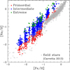 |
Fig. 1 Fractions of stars with primordial (P, red circles), intermediate (I, blue circles), and extreme (E, green circles) composition in our programme GCs, superimposed to a reference sample of unpolluted field stars from Carretta (2013, : grey open triangles). |
2 Analysis
The spectroscopic material is described in Carretta et al. (2009a,b). Briefly, for GIRAFFE spectra we used the two highresolution setups HR11 (spectral resolution R = 24 200, centred on 5728 Å) and HR13 (R = 22 500, centred at 6273 Å). The UVES Red Arm fed by FLAMES fibres (up to a maximum of 7 per fibre positioning configuration) covers a spectral range of 4800-6800 Å with a resolution R ≃ 45 000. All targets were selected among isolated stars near the RGB ridge line in each GC.
We adopted the atmospheric parameters derived in Carretta et al. (2009a,b) and the iron ratios [Fe/H] from Carretta et al. (2009c) for all the stars analysed. Line lists, atomic parameters, and solar reference abundances (from Gratton et al. 2003) are strictly homogeneous with all the previous studies from our group.
Abundances of Mg, Si, Ca, and Ti were derived from equivalent widths (EWs) measured with the ROSA package (Gratton 1988) as described in detail in Bragaglia et al. (2001). Following the procedure adopted by Carretta et al. (2009a), stars observed in each GC with both spectrographs were used to register the EWs from GIRAFFE to those measured on the higher resolution UVES spectra.
For titanium, neutral transitions are available both in UVES and in GIRAFFE spectra. In addition, also singly ionised transitions could be measured for the few UVES stars in each GC of the sample. We found on average [Ti/Fe] I - [Ti/Fe] II = -0.008 ± 0.004 dex (σ = 0.050 dex, 188 stars). The excellent match between [Ti/Fe] I and [Ti/Fe] II is a safety check on the reliability of the analysis and on the adopted scale of atmospheric parameters, in particular the surface gravity. If not stated otherwise, in the following, for titanium we use the average abundance of [Ti/Fe] I, derived from much larger samples of stars in each GC.
A second critical check consists of looking for trends in the abundances as a function of temperature. Several signatures of MPs in GCs involve correlations and anti-correlations among different species produced and destroyed in proton-capture reactions. Hence, it is crucial to verify that in the data there are no spurious trends due to some temperature-dependent errors from the abundance analysis.
In Fig. B.1, we plot the abundances of Mg, Si, Ca, [Ti/Fe] I and [Ti/Fe] II for all stars analysed in the 16 programme GCs as a function of the effective temperature (Teff). The vertical scale is determined by the specie with the largest observed dispersion (Mg in NGC 7078). The blue squares are UVES stars, and the red circles are for GIRAFFE stars. For each abundance ratio in each GC, we computed the linear regression as a function of temperature. Out of 80 cases, the relation is statistically significant only for Mg and Si for NGC 6752 (from Carretta et al. 2012), and for Si in NGC 6171 and NGC 6809 from the present work. These trends may help explain the larger offset in UVES and GIRAFFE abundances in NGC 6752 (see Table A.1). However, the average ratios in different temperature bins differ only by a few hundredths of dex even in these cases (with a maximum of 0.07 and 0.08 dex in NGC 6752); therefore, they do not significantly affect our following results. Since there are no significant gradients with temperature, this is a rather robust safety check on our analysis. Since there are no significant offsets, we are entitled to safely merge the UVES and GIRAFFE samples. For stars studied in both samples, however, we privileged the UVES abundances, which generally are based on a larger number of lines.
The average results are listed in Table A.1. In the first line for each element in each GC we report the average abundance and the rms scatter from the UVES sample, together with the cluster metallicity from Carretta et al. (2009c). The second line is for the abundances from GIRAFFE, and in the third line we list the results of the merging of the two previous sets, that is, the unique stars in each GC. In the present paper, we provide a measurement of some α-elements (not previously published) for slightly more than 1500 RGB stars.
The abundances of α-elements for individual stars are available in electronic form at CDS. We provide star identification, coordinates, number of lines, average abundance, line-to-line scatter, and a flag (UVES or GIRAFFE) for each element.
2.1 Error budget
The error budget was estimated as described in detail in Carretta et al. (2009b,a) for abundances derived from UVES and GIRAFFE spectra, respectively. To obtain the star to star errors, two ingredients are necessary: a fair estimate of the internal errors in the atmospheric parameters (as well as in the EW measurement) and the sensitivity, that is, the change in the abundance ensuing a variation in one of the parameters. Internal errors are estimated and tabulated in Carretta et al. (2009a) and Carretta et al. (2009b) for the GIRAFFE and UVES samples, respectively.
To derive the sensitivity of the derived abundances on the adopted atmospheric parameters, we repeated the abundance analysis by changing only one parameter (effective temperature, surface gravity) each time for all stars in a GC. The sensitivity to each parameter was adopted as the average of all the stars over the sampled temperature range. This procedure was repeated separately for the UVES and GIRAFFE samples in each programme GC.
The sensitivity of Mg, Si, Ca, [Ti/Fe] I, and [Ti/Fe] II in response to the amount of changes in the parameters listed in the table header are reported in Tables C.1 and C.2 for UVES and GIRAFFE, respectively. By multiplying the sensitivity of each element for the internal errors in the parameters, we obtained the internal errors in abundances due to internal errors in the adopted parameters.
The resulting errors, the average number of lines for each species, and the error estimates due to measurement errors in the EW are listed for all GCs in Table C.3. We obtained the estimated internal errors listed in the table by summing in quadrature all the contributions.
2.2 Comparison with other spectroscopic surveys
We compared our results with other large surveys using stars in common. With the Gaia-ESO (GES) Survey final data release DR5.1 (Gilmore et al. 2022; Randich et al. 2022) we have in common 232 stars in six GCs and 68 stars when considering only the UVES U580 setup, with large spectral coverage, in GES. The mean temperature offset (this work minus GES) is -65.1 K (σ = 160.7 K, total sample) or -183.5 K (σ = 138.2 K, UVES). The corresponding offsets in surface gravity are +0.12 dex (σ = 0.49 dex, total) and -0.15 dex (σ = 0.36 dex, UVES). After bringing the GES data to our scale of solar abundances, the offsets in [Fe/H] are +0.095 dex (σ = 0.136 dex), decreasing to +0.071 dex (σ = 0.105 dex), when using only the U580 setup in GES.
The comparison for all the analysed elements is shown as a function of the effective temperature in Fig. D.1 for the stars in common in the six GCs. All abundance ratios from GES were shifted to our scale. The filled points for GES represent the U580 setup. If we restrict to the four GCs with sufficient stars observed with the U580 setup, our abundances have an offset on average within ±0.1 dex from the mean abundances from GES, except for Ca. However, the star to star scatter is noticeably larger for all the analysed species in GES data. On average, in NGC 104, NGC 1904, NGC 6752, and NGC 7078 the rms scatter of the mean is 0.147 dex, 0.105 dex, 0.133 dex, and 0.189 dex for Mg, Si, Ca, and Ti in GES to be compared with the averages 0.096 dex, 0.062 dex, 0.037 dex, and 0.034 dex for the corresponding stars in the present work. Looking at Fig. D.1, this is probably due to the significant trends as a function of the temperature present in the GES data in several cases, even when only the more reliable U580 dataset is considered, suggesting problems in the set of atmospheric parameters or in the procedure used in the GES analysis.
We have 321 stars in common in nine GCs with the GALactic Archaeology with HERMES (GALAH) survey DR4 (Buder et al. 2025). After excluding unreliable stars using the prescribed criteria from the GALAH website2, to retain only stars with reliable spectroscopic analysis and abundances, the mean offsets in temperature and gravity are -67.3 K (σ = 95.3 K) and -0.054 dex (σ = 0.060 dex) for 158 stars. We used the values in table C.1 by Buder et al. (2025) to correct the GALAH abundances to our scale. The comparison of the abundances as a function of the temperature for the stars in common is shown in Fig. D.2. Overall, there is reasonable agreement in both mean value and scatter. The mean offsets (this work minus GALAH) are -0.016 dex, -0.003 dex, -0.124 dex, and -0.065 dex for Mg, Si, Ca, and Ti. The average rms scatter in GALAH is 0.059 dex, 0.041 dex, 0.100 dex, and 0.101 dex, respectively, to be compared with 0.056 dex, 0.041 dex, 0.034 dex, and 0.038 dex for stars in common with the present work.
With the recommended selection criteria (STARFLAG=0, ASPCAPFLAG=0), we found 373 stars in common in 15 GCs with the Apache Point Observatory Galactic Evolution Experiment (APOGEE) DR17 (Abdurro’uf et al. 2022). The mean offsets are -162.2 K (σ = 107.0 K) in temperature, -0.055 dex (σ = 0.146 dex) in gravity, and -0.115 dex (σ = 0.103 dex) in [Fe/H]. The comparison of the abundances, in Fig. D.3, is done using the original APOGEE abundances since no solar abundances are explicitly stated for that survey. Our abundances of α-elements from optical spectra are systematically larger than those derived by APOGEE near-infrared spectra. On average we found offsets (this work minus APOGEE) of +0.212 dex (σ = 0.081 dex, 358 stars) for Mg, +0.157 dex (σ = 0.086 dex, 358 stars) for Si, +0.127 dex (σ = 0.121 dex, 358 stars) for Ca, and +0.172 dex (σ = 0.127 dex, 333 stars) for Ti I. The best agreement is found for Ti II (-0.007 dex), although with a large scatter (σ = 0.171 dex, 75 stars). The average rms scatter is 0.064 dex, 0.042 dex, 0.121 dex, 0.132 dex, and 0.136 dex for Mg, Si, Ca, Ti I, and Ti II in APOGEE to be compared with average values 0.067 dex, 0.043 dex, 0.038 dex, 0.039 dex, and 0.025 dex in the present work.
3 Results: the general pattern
The average abundances of individual α-elements are shown in Fig. 2 as a function of the metallicity [Fe/H]. Filled points are the 16 programme GCs in the present paper, while empty circles are GCs from previous studies of individual GCs, summarised in Table 1 together with the mean metallicity of UVES to locate them in the plots. The methodology of the abundance analysis being identical, this addition provides an extended sample which is very homogeneous, improving the statistics. The red colour is used for in situ GCs and the blue colour indicates accreted GCs. For this classification, we follow the associations given in Massari et al. (2019). For GCs with uncertain progenitors (NGC 3201, NGC 5904, NGC 5634, and NGC 6535) we adopt the associations for which both Forbes (2020) and Callingham et al. (2022) agree, that is, Sequoia for NGC 3201 and NGC 6535, and Helmi streams for NGC 5904 and NGC 5634. Empty grey circles are Milky Way field stars used as a comparison. We adopted the sample from Gratton et al. (2003), which is a mixture of the dissipational and accreted components in the Galaxy because that study used the same line list and solar abundances as the present work.
In Fig. 2, we plot the average abundances of «-elements as a function of the metallicity. The ratios [Mg/Fe] and [Si/Fe] are roughly constant up to the metallicity of our most metal-rich object, NGC 6441. This pattern is consistent with a constant level of Mg shared also by disk and bulge GCs with abundances derived from optical spectroscopy in the literature (e.g. Muñoz et al. 2017, 2018, 2020; Mura-Guzmán et al. 2018; Puls et al. 2018). For Si, a decrease after the knee located at [Fe/H] ~ -1 dex is not found in our data, and is apparent only in low-mass bulge GCs (Muñoz et al. 2018, 2020) from optical spectroscopy, whereas in APOGEE data Si is clearly decreasing (e.g. H20). In the present work, a decrease in the average abundances is observed only for Ca. The average abundances of GCs are mostly comparable to those of field stars, with the exception of Si in NGC 6441.
Moreover, for most elements, we found no significant differences between the distribution of ex situ and that of in situ GCs. Comparing the 19 ex situ GCs and the eight in situ GCs with a Kolmogorov-Smirnov (K-S) test, we could not safely reject the null hypothesis that the two distributions are extracted from the same parent population looking at the average abundances of Mg, Si, Ca, and Ti (p-value 0.41, 0.27, 0.74, and 0.06, respectively, with the usual 0.05 threshold for significance).
Our findings do not agree with the conclusions of Horta et al. (2020, H20). Using the average Si abundances from APOGEE DR17 for 46 GCs, they claim that there is a distinction between in situ and accreted GCs, at least in the metallicity range of [Fe∕H]=-1.5 to -1 dex, with the in situ subgroup displaying a higher [Si/Fe] average abundance. In our data a K-S test for [Si/Fe] over metallicity -1.5 < [Fe/H] < -1, where according to H20 the difference between the in situ and accreted GCs is most evident, returns a two-tailed probability p=0.49.
Their work is the only one, to our knowledge, to provide tabulated average [Si/Fe] abundances from APOGEE for the analysed GCs, and we have 20 GCs in common between our sample (enlarged with the addition of previous homogeneous studies in Table 1) and H20.
The offset in metallicity is scarcely significant. We found on average that [Fe/H]thiswork - [Fe/H]APOGEE = -0.063 ± 0.016 dex with σ = 0.073 dex (20 GCs). The actual difference lies in the Si abundances, and the comparison is shown in Fig. 3.
Computed on 20 GCs, the abundance [Si/Fe] derived in the present work is on average higher than those used by H20 by 0.162 dex (σ =0.075 dex), in agreement with what is found in Section 2.2. However, more importantly, this offset is not constant but varies as a function of metallicity, with a clear trend to increase as [Fe/H] increases.
Since the GCs formed in situ (either in the main disc or in the main bulge of the progenitor Galaxy) are on average more metal-rich than those formed ex situ, the discrepancy in the Si abundances increases when the majority of GCs are not accreted, in the metallicity regime ≳-1.2 dex. This trend may explain the different conclusions reached by H20 and the present study, as well as the large discrepancy between the APOGEE [Si/Fe] average for NGC 6388 and the abundance given by Carretta & Bragaglia (2023)3. However, internal errors in the [Si/Fe] ratio in both the present work and APOGEE are close to the difference claimed from the accreted and in situ GCs (about 0.1 dex). This evidence, coupled with possible systematic offsets, would require even more precise abundances for a definitive answer to this issue.
Finally, our data do not seem to confirm a tension between the kinematics of NGC 288 and its chemistry, as advocated by H20 from the abundances in APOGEE. Although the orbital parameters unambiguously associate NGC 288 with the Gaia-Enceladus (GE) accretion event, H20 finds that the level of α-elements in this GC is much higher than in other candidate GE GCs and is more in agreement with other GCs originated in situ. In our analysis, the [Mg/Fe] ratio of NGC 288 is in agreement with that of other GCs associated with GE (blue points in Fig. 4), but also compatible with the abundance of in situ GCs. The same is even more true for the Si abundance, whereas the Ca abundance in NGC 288 is marginally higher than in other clusters from GE. We must conclude that in both the present work and in APOGEE there is no strong evidence favouring the attribution of NGC 288 to in situ or to GE groups from chemical abundances alone.
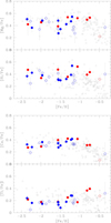 |
Fig. 2 Average abundance ratios [Mg/Fe], [Si/Fe], [Ca/Fe], [Ti/Fe] I as a function of metallicity [Fe/H], with the 1σ spread represented as error bars. Filled symbols are for the 16 GCs of the present work, empty symbols indicate GCs from previous individual studies. Red and blue colours are for in situ and ex situ GCs, respectively. Grey points are field stars from Gratton et al. (2003). |
GCs from previous studies.
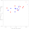 |
Fig. 3 Differences of the average [Si/Fe] abundance from this work (extended sample) and APOGEE (from Horta et al. 2020) for 20 GCs in common. Symbols are as in Fig. 2. |
4 Temperature tomography of multiple populations
With abundances of α-elements in several hundreds of stars, we have a sample well suited to investigate the different temperature regimes in which proton-capture reactions were activated in GCs. More or less energetic reactions being active in stars of different mass ranges, this study may provide useful constraints to tune models of cluster formation and evolution.
4.1 The high temperature regime: Mg and Si
A complete survey of O, Na, Mg, Al, and Si and their interrelated abundances was done in Carretta et al. (2009b), but only for a limited sample in each GC (a maximum of 14 stars, those observed with the UVES Red-arm fibres). Despite the small sample size, the discovery that a clear Mg-Al anti-correlation (produced at temperatures ≳70 MK, see e.g., Prantzos et al. 2017; Gratton et al. 2019) is only detectable in metal-poor or massive GCs dates from that study. In the present study, we do not have abundances of Al available for all stars, but we are able to test variations in Mg and Si.
Despite the generally small variations in these species, dwarfed, for example, by changes in O, Na, and Al, a first indication comes from even considering the average [element/Fe] ratios, as in Fig. 5. In the three panels, the mean values [Mg/Fe] and [Si/Fe] are re-computed again for all GCs using only stars of the primordial P component (left panel), and the stars of the polluted populations with intermediate I and extreme E composition (middle and right panels, respectively). The E component, however, is not present in all GCs. When using as reference the line traced on the upper envelope distributions of Mg and Si in the left panel, it is easy to see that Mg is decreasing and Si slightly increasing proceeding towards stars with more and more altered composition, that is, along the sequence P-I-E.
More quantitative statistics are represented in Fig. 6. We applied a K-S test to the cumulative distributions of the ratios [Mg/Fe], [Si/Fe], and [Mg/Si] in the P, I, and E components in the 16 programme GCs. For each ratio, it was possible to safely reject the null hypothesis that the samples are extracted from the same parent population, at least in terms of the polluted and unpolluted components, since variations in Mg and Si are not equally pronounced in all GCs.
We also know that Na and O are modified in practically all GCs (e.g. Carretta et al. 2009a,b, 2010a for extensive surveys), and the changes in [Mg/Na] and [Si/Na] are probably driven by the large variations in the Na content among the P, I, and E components. For a more detailed screening it is possible to see in which GCs Mg is more involved in MPs by evaluating the anti-correlation with Na or the Mg-O correlation. In Fig. 7 we plot the results for the six GCs where a linear regression is statistically significant (p-value<0.05), according to the Pearson’s correlation coefficient and the two-tailed probability that the correlation is real, both listed in each panel. The Mg-Na anticorrelation is matched rather well by the complementary Mg-O correlation4, but the first relation represents a better indication because Na is available for many more stars than O.
We confirm the discovery made by Carretta et al. (2009b) that the largest star to star variations in the Mg abundance are found among the MPs of metal-poor and massive GCs. The conclusion in the present study is based on a sample more than a factor 6 larger than the sample used by Carretta et al. (2009b).
The distributions of the [Mg/Si] ratios are much closer to each other than those including the specie with the largest variation (Na), as expected from the involved mechanism that is a simple leakage from the main MgAl cycle (e.g. Yong et al. 2005; Carretta et al. 2009b). In our data, 10 out of 16 GCs show a statistically significant correlation Si-Na (Fig. 8). For the other six GCs, the probabilities of linear regression are p=0.71, 0.08, 0.15, 0.07, 0.07, and 0.66 (for NGC 3201, NGC 4590, NGC 6171, NGC 6397, NGC 6809, and NGC 6838, respectively). This evidence suggests that leakage from Mg to Si is not a relevant phenomenon in these GCs.
 |
Fig. 4 Abundance ratios [Mg/Fe], [Si/Fe], and [Ca/Fe] as a function of the orbital energy of the GCs, from Savino, & Posti (2019). Red and blue symbols are for GCs formed in situ and associated with Gaia-Enceladus. Filled and empty circles refer to the present and previous works, respectively. In each panel, the abundance level of NGC 288 is indicated by the vertical line. |
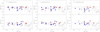 |
Fig. 5 Average abundance ratios [Mg/Fe] and [Si/Fe] for GCs in our extended sample, using only the unpolluted P fraction (left panel), the polluted component with intermediate I and extreme E composition (middle and right panel, respectively) in each GC. The horizontal lines trace by eye the upper envelope of abundances in the left panel and are reproduced in the other two panels. |
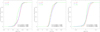 |
Fig. 6 Results of the Kolmogorov-Smirnov test on the cumulative distributions of the [Mg/Fe], [Si/Fe], and [Mg/Si] of the P, I, and E components in the 16 programme GCs. In each panel the probability of the K-S test for the comparison P-I and P-E is listed. |
 |
Fig. 7 The Na-Mg anti-correlation in the GCs of our programme sample where the linear regression between Na and Mg is found to be statistically significant (p-value < 0.05). The Pearson’s correlation coefficient and probability are listed in each panel together with a typical error bar. |
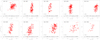 |
Fig. 8 The Si-Na correlation in the GCs of our programme sample where the linear regression is found to be statistically significant. A typical error bar is shown. |
4.2 The very high temperature regime: Ca
The regime of MPs with chemistry generated by proton-capture reactions at very high temperatures can be studied with the aid of the diagnostic plot introduced in Carretta et al. (2013c), measuring possible excesses of Ca linked to Mg depletions. In this regime, the normal production of Al from Mg destruction may be bypassed favouring the production of heavier species such as K, Ca, and even Sc from proton-captures in Ar nuclei (Ventura et al. 2012). The Ca and Mg abundances measured for a large number of stars in the present work provide useful statistics to investigate the relevance of these very high temperature nuclear cycles involved in polluters of the first stellar generation in GCs (see also Carretta & Bragaglia 2021 and references therein). In Fig. 9, we plot the abundance ratio [Ca/Mg] as a function of the [Ca/H] ratio for all stars in the 16 programme GCs.
In the left panel of Fig. 9 we superimposed the stars in NGC 2808 (green filled circles) from Carretta (2015). In the MPs of this GC, correlations and anti-correlations with Mg are observed up to the heaviest proton-capture species, like K (Mucciarelli et al. 2015), Ca and Sc (Carretta 2015). The large extension of the [Ca/Mg] ratios is explained by large depletions in Mg accompanied by moderate excesses in the Ca content.
In the middle and right panels, our strictly homogeneous analysis allows us to highlight the same behaviour also for stars in NGC 6752 and NGC 7078, although to a lesser extent. These are the only two GCs in our present sample where a significant excess in the [Ca/Mg] ratio was observed. The depletion in Mg was already assessed in previous sections. To check whether the depletion in Mg is also matched by a slight enhancement in the Ca abundance, we resort to the procedure used in Carretta & Bragaglia (2021). In their systematic survey to find an excess of Ca and Sc in GC stars, they used as a reference the same sample of unpolluted field stars from Gratton et al. (2003) used in the present work. The differential procedure compares in the plane [Ca/H]-[Mg/H] GC stars with the abundance pattern of field stars that are expected to incorporate only the yields from supernova nucleosynthesis.
We repeated the steps used by Carretta & Bragaglia 2021 on all the GCs of their silver sample, that is, the homogeneously analysed but limited samples of stars observed with the dedicated UVES-FLAMES fibres in Carretta et al. (2009b). In the present analysis, we significantly increased the samples by also exploiting the homogeneous analysis of the GIRAFFE spectra. The results found to be statistically significant are illustrated in Fig. 10. Stars in NGC 6752 and NGC 7078 (blue squares) are superimposed on field stars from Gratton et al. (2003, empty grey squares) in the [Ca/H]-[Mg/H] plane (upper left panels). We then subtract the linear fit traced to field stars from both samples to obtain linearised [Ca/H]corr values, for an easier evaluation of excesses (upper right panels). The generalised histograms in the lower left panels, aligned using the mode of the distributions, allow us to estimate the excess of [Ca/H] of GC stars with respect to the reference sample of unpolluted field stars. Finally, a K-S test is applied to the cumulative distributions of field and GC stars in the lower right panels. The two-tailed probability is listed. Despite the evidence in Fig. 9 and the excess (although small) shown in Fig. 10, the value of NGC 6752 does not allow us to safely reject the null hypothesis that the two samples are extracted from the same parent population. Rather, the test is even formally significant in the case of NGC 7078, indicating an excess of Ca together with a depletion of Mg and signalling the outcome of proton-capture reactions under the very high temperature regime.
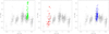 |
Fig. 9 Diagnostic plot [Ca/Mg] as a function of [Ca/H] for the stars of 16 GCs in the present study (empty grey points). In the left panel, green filled circles are stars in NGC 2808 from Carretta 2015, in the middle and right panels, red and blue filled circles are stars in NGC 7078 and NGC 6752, respectively, from the present work. |
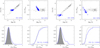 |
Fig. 10 Detection of Ca excesses in NGC 6752 (left panels) and NGC 7078 (right panels). In the upper left panels GC stars (blue squares) are superimposed to field stars (with typical error of 0.08 dex), and all abundances are linearised in the upper right panels (see text). Generalised histograms of the [Ca/H] values for field (grey area) and GC stars (blue area) are in the lower left panels and the cumulative distributions are shown in the lower right panels, together with the probability of the two-tailed K-S test. |
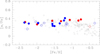 |
Fig. 11 Ratios [α/Fe] (average of [Si/Fe], [Ca/Fe], [Ti/Fe]) as a function of metallicity. Grey circles are field stars from Gratton et al. (2003). Blue and red filled circles are accreted and in situ GCs in our extended sample. |
5 Discussion and summary
In the present work, we derived homogeneous abundances of Mg, Si, Ca, and Ti for a large sample of RGB stars in 16 GCs that cover most of the metallicity range of Milky Way GCs. Thanks to the identical methodology used in the analysis, the sample can be safely coupled to previous studies of individual GCs by our group, assembling one of the largest samples of giants (more than 2600) in GCs with abundances from high resolution optical spectra. The extremely homogeneous analysis minimises possible systematics.
In our data, the abundance of α-elements is found to be approximately constant in all GCs studied (Fig. 2). This is more evident in Fig. 11 where we show the mean < [«/Fe]> ratio computed as the average of [Si/Fe], [Ca/Fe], and [Ti/Fe], the three elements that are the least affected by the abundance variations related to MPs. The ratio < [«/Fe]> is flat as a function of [Fe/H] up to the metallicity of the GCs in the MW bulge (NGC 6388 and NGC 6441). The signature of type Ia SNe (lower < [«/Fe]>) is not apparent in all GCs examined here, whereas the classical downturn at [Fe/H]=-1 dex is seen among field stars and in the [Si/Fe] ratios of APOGEE.
Thus, the constancy of «-elements in GCs born in a variety of environments implies that the effects of SN Ia are never seen in individual GCs, apart from a few notable cases like ω Cen (see Gratton et al. 2004). Observationally, this is supported by the small dispersions in [Fe/H] in almost all GCs (see e.g. Carretta & Bragaglia 2025; Latour et al. 2025). The main origin theories for MPs in GCs suggest that the formation of polluted stars occurs on very short timescales (a few million years) for enrichment from massive stars (e.g. Gieles et al. 2025), reaching up to 80-100 Myr for the asymptotic giant branch stars (AGB), as this is the timescale for the first SNe Ia to stop further generations of stars forming within the cluster (D’Ercole et al. 2008). The near homogeneity of heavy elements in GCs suggests that these objects were already gas free when SNe exploded or gas was lost following the explosions. Analytical models computed to reproduce the observed metallicity spreads advocate that star formation ended in GCs after 3-4 Myr (Wirth et al. 2022); hence most of the enrichment should take place within a few Myr, well before the explosions of the first thermonuclear SNe.
The scatter in the mean values in Fig. 2 is compatible with a stochastic enrichment from a few core-collapse SNe, as first noted by Carney (1996). This is the main reason why the origin of in situ and accreted GCs cannot be recognised from the abundance of «-elements alone.
In more than half of the GC sample we found star to star variations in Si correlated to changes in the Na abundance. This evidence, corroborated by robust statistical tests, indicates that in these GCs the stars enriching the gas that formed the polluted population reached temperatures high enough for a significant leakage from the MgAl chain on 28 Si. According to models based on rates from NACRE (Arnould et al. 1999), this implies exceeding a threshold temperature of about 65 MK in these still unidentified sources of proton-capture reactions. From our current data, this seems to be a rather common occurrence.
The presence of large changes in the Mg abundance established by core-collapse SNe is less frequent. Significant variations in Mg are only found in GCs that are metal-poor, massive, or both (like NGC 7078, where a few stars show [Mg/Fe]<0.0), confirming the early findings by Carretta et al. (2009b), and later additional evidence (e.g. Mészáros et al. 2020), on a more statistically robust sample. However, the higher temperatures involved in the MgAl chain with respect to those required to produce the widespread Na-O anti-correlation and the much larger primordial abundances of Mg and Si in GC stars imply that MPs have a small impact on the average abundances of «-elements in GCs.
Finally, we found the signature of the action of protoncapture reactions at a very high temperature in two out of 16 GCs. Following the approach detailed in Carretta & Bragaglia (2021) we detected excesses of Ca with respect to field stars of similar metallicity in NGC 6752 and NGC 7078. These excesses possibly trace the production of Ca activated on Ar nuclei by proton capture in a particularly energetic regime (Ventura et al. 2012). When testing the null hypothesis that the sample populations of GC stars and unpolluted field stars are drawn from the same parent distribution, a K-S test unambiguously shows that the result for NGC 7078 is of high significance. The case of NGC 6752 is formally not statistically significant. However, the excess can be quantified by computing the number of outliers in the linearised GC distribution. Following Carretta & Bragaglia (2021), outliers are defined as those whose corrected ratios [Ca/H]corr exceed the 3σ range with respect to the average for field stars. The measured fractions of outliers (0.098 for NGC 6752 and 0.259 for NGC 7078) fit very well the relation with a linear combination of cluster mass and metallicity found in Carretta & Bragaglia (2021). In Fig. 12 we plot in red the eight GCs where a significant excess of Ca was found by Carretta & Bragaglia (2021). By adding the GCs from the present work (blue points) we repeated the fit, finding a correlation with very high significance, as indicated by the two-tailed probability listed in the figure, with a net improvement from the p-value (3.0 × 10⁻⁴) found in Carretta & Bragaglia (2021).
The dependence on global cluster mass and metallicity is the same combination that affects other characteristics of MPs in GCs such as the amount of Al produced in polluters (Carretta et al. 2009b) or the minimum abundance of O observed in GCs [O/Fe]min (Carretta et al. 2009a). This bivariate dependence seems to be thus effective in driving the behaviour of MPs (Na-O and Mg-Al anti-correlations, Ca excesses) over several regimes distinguished by the involved temperature range in the putative polluters.
The era of artisanal abundance surveys is ending. Forthcoming large-scale spectroscopic surveys, such as 4MOST and WEAVE, will deliver high-quality data for millions of stars and a large fraction of Galactic stellar clusters. Our precise, large, and very homogeneous sample of giant stars in GCs, all certified members by radial velocity and abundance, may be a useful benchmark for these ’industrial’ surveys, contributing to their calibration and validation.
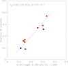 |
Fig. 12 Fraction of stars with excesses of Ca in 8 GCs from the census in Carretta & Bragaglia (2021, red points)) as a function of a linear combination of GC mass (Baumgardt et al. 2019) and metallicity (Harris 2010). Blue points are for NGC 7078 and NGC 6752 from the present work. A linear fit is given by the solid line, with the Pearson’s correlation coefficient and the two-tailed probability listed in the panel. |
Data availability
Abundances for individual stars are available at the CDS via https://cdsarc.cds.unistra.fr/viz-bin/cat/J/A+A/707/A322.
Acknowledgements
This research has made large use of the SIMBAD database (in particular Vizier), operated at CDS, Strasbourg, France, of the NASA’s Astrophysical Data System, and TOPCAT (Taylor 2005). I especially thanks Angela Bragaglia for several valuable suggestions. I also aknowledge funding from Bando Astrofisica Fondamentale INAF 2023 (PI A. Vallenari) and from Prin INAF 2019 (PI S. Lucatello).
References
- Abdurro’uf, Accetta, K., Aerts, C., et al. 2022, ApJS, 259, 35 [NASA ADS] [CrossRef] [Google Scholar]
- Adamo, A., Bradley, L. D., Vanzella, E., et al. 2024, Nature, 632, 513 [NASA ADS] [CrossRef] [Google Scholar]
- Arnould, M., Goriely, S., & Jorissen, A. 1999, A&A, 347, 572 [NASA ADS] [Google Scholar]
- Bastian, N., & Lardo, C. 2018, ARA&A, 56, 83 [Google Scholar]
- Baumgardt, H., Hilker, M., Sollima, A., & Bellini, A. 2019, MNRAS, 482, 5138 [Google Scholar]
- Bragaglia, A., Carretta, E., Gratton, R. G., et al. 2001, AJ, 121, 327 [NASA ADS] [CrossRef] [Google Scholar]
- Bragaglia, A., Carretta, E., D’Orazi, V., et al. 2017, A&A, 607, A44 [NASA ADS] [CrossRef] [EDP Sciences] [Google Scholar]
- Buder, S., Kos, J., Wang, X. E., et al. 2025, PASA, 42, 51 [Google Scholar]
- Callingham, T. M., Cautun, M., Deason, A. J., et al. 2022, MNRAS, 513, 4107 [NASA ADS] [CrossRef] [Google Scholar]
- Carney, B. W. 1996, PASP, 108, 900 [Google Scholar]
- Carretta, E. 2013, A&A, 557, A128 [NASA ADS] [CrossRef] [EDP Sciences] [Google Scholar]
- Carretta, E. 2015, ApJ, 810, 148 [Google Scholar]
- Carretta, E. 2021, A&A, 649, A154 [NASA ADS] [CrossRef] [EDP Sciences] [Google Scholar]
- Carretta, E. 2022, A&A, 666, A177 [NASA ADS] [CrossRef] [EDP Sciences] [Google Scholar]
- Carretta, E., & Bragaglia, A. 2021, A&A, 646, A9 [EDP Sciences] [Google Scholar]
- Carretta, E., & Bragaglia, A. 2022, A&A, 660, L1 [NASA ADS] [CrossRef] [EDP Sciences] [Google Scholar]
- Carretta, E., & Bragaglia, A. 2023, A&A, 677, A73 [NASA ADS] [CrossRef] [EDP Sciences] [Google Scholar]
- Carretta, E., & Bragaglia, A. 2025, A&A, 696, A120 [NASA ADS] [CrossRef] [EDP Sciences] [Google Scholar]
- Carretta, E., Bragaglia, A., Gratton, R. G., et al. 2006, A&A, 450, 523 [NASA ADS] [CrossRef] [EDP Sciences] [Google Scholar]
- Carretta, E., Bragaglia, A., Gratton, R. G., et al. 2009a, A&A, 505, 117 [NASA ADS] [CrossRef] [EDP Sciences] [Google Scholar]
- Carretta, E., Bragaglia, A., Gratton, R. G., & Lucatello, S. 2009b, A&A, 505, 139 [NASA ADS] [CrossRef] [EDP Sciences] [Google Scholar]
- Carretta, E., Bragaglia, A., Gratton, R. G., D’Orazi, V., & Lucatello, S. 2009c, A&A, 508, 695 [NASA ADS] [CrossRef] [EDP Sciences] [Google Scholar]
- Carretta, E., Bragaglia, A., Gratton, R. G., et al. 2010a, A&A, 516, 55 [Google Scholar]
- Carretta, E., Bragaglia, A., Gratton, R. G., et al. 2010b, ApJ, 712, L21 [Google Scholar]
- Carretta, E., Bragaglia, A., Gratton, R. G., et al. 2010c, A&A, 520, 95 [Google Scholar]
- Carretta, E., Lucatello, S., Gratton, R. G., Bragaglia, A., & D’Orazi, V. 2011, A&A, 533, 69 [Google Scholar]
- Carretta, E., Bragaglia, A., Gratton, R. G., Lucatello, S., & D’Orazi, V. 2012, ApJ, 750, L14 [NASA ADS] [CrossRef] [Google Scholar]
- Carretta, E., Gratton, R. G., Bragaglia, A., D’Orazi, V., & Lucatello, S. 2013a, A&A, 550, A34 [NASA ADS] [CrossRef] [EDP Sciences] [Google Scholar]
- Carretta, E., Bragaglia, A., Gratton, R. G., et al. 2013b, A&A, 557, A138 [NASA ADS] [CrossRef] [EDP Sciences] [Google Scholar]
- Carretta, E., Gratton, R. G., Bragaglia, A., et al. 2013c, ApJ, 769, 40 [Google Scholar]
- Carretta, E., Bragaglia, A., Gratton, R. G., et al. 2014a, A&A, 564, A60 [NASA ADS] [CrossRef] [EDP Sciences] [Google Scholar]
- Carretta, E., Bragaglia, A., Gratton, R. G., et al. 2014b, A&A, 561, A87 [NASA ADS] [CrossRef] [EDP Sciences] [Google Scholar]
- Carretta, E., Bragaglia, A., Gratton, R. G., et al. 2015, A&A, 578, A116 [CrossRef] [EDP Sciences] [Google Scholar]
- Carretta, E., Bragaglia, A., Lucatello, S., et al. 2017, A&A, 600, A118 [NASA ADS] [CrossRef] [EDP Sciences] [Google Scholar]
- Cohen, J. G., & Kirby, E. N. 2012, ApJ, 760, 86 [Google Scholar]
- D’Ercole, A., Vesperini, E., D’Antona, F., McMillan, S. L. W., & Recchi, S. 2008, MNRAS, 391, 825 [CrossRef] [Google Scholar]
- Eggen, O. J., Lynden-Bell, D., & Sandage, A. R. 1962, ApJ, 136, 748 [NASA ADS] [CrossRef] [Google Scholar]
- Forbes, D. A. 2020, MNRAS, 493, 847 [Google Scholar]
- Gieles, M., Padoan, P., Charbonnel, C., Vink, J. S., & Ramirez-Galeano, L. 2025, MNRAS, 544, 483 [Google Scholar]
- Gilmore, G., Randich, S., Worley, C. C., et al. 2022, A&A, 666, A120 [NASA ADS] [CrossRef] [EDP Sciences] [Google Scholar]
- Gratton, R. G. 1988, Rome Obs. Preprint Ser., 29 [Google Scholar]
- Gratton, R. G., Carretta, E., Claudi, R., Lucatello, S., & Barbieri, M. 2003, A&A, 404, 187 [NASA ADS] [CrossRef] [EDP Sciences] [Google Scholar]
- Gratton, R. G., Sneden, C., & Carretta, E. 2004, ARA&A, 42, 385 [Google Scholar]
- Gratton, R. G., Lucatello, S., Bragaglia, A., et al. 2006, A&A, 455, 271 [NASA ADS] [CrossRef] [EDP Sciences] [Google Scholar]
- Gratton, R. G., Lucatello, S., Bragaglia, A., et al. 2007, A&A, 464, 953 [NASA ADS] [CrossRef] [EDP Sciences] [Google Scholar]
- Gratton, R. G., Carretta, E., & Bragaglia, A. 2012, A&ARv, 20, 50 [CrossRef] [Google Scholar]
- Gratton, R. G., Bragaglia, A., Carretta, E., et al. 2019, A&ARv, 27, 8 [Google Scholar]
- Harris, W. E. 2010, [arXiv:1012.3224] [Google Scholar]
- Horta, D., Schiavon, R. P., Mackereth, J. T., et al. 2020, MNRAS, 493, 3363 [NASA ADS] [CrossRef] [Google Scholar]
- Kraft, R. P. 1994, PASP, 106, 553 [Google Scholar]
- Langer, G. E., Hoffman, R., & Sneden, C. 1993, PASP, 105, 301 [NASA ADS] [CrossRef] [Google Scholar]
- Latour, M., Kamann, S., Martocchia, S., et al. 2025, A&A, 694, A248 [NASA ADS] [CrossRef] [EDP Sciences] [Google Scholar]
- Massari, D., Koppelman, H. H., & Helmi, A. 2019, A&A, 630, L4 [NASA ADS] [CrossRef] [EDP Sciences] [Google Scholar]
- Mészáros, S., Masseron, T., García-Hernández, D. A., et al. 2020, MNRAS, 492, 1641 [Google Scholar]
- Mucciarelli, A., Bellazzini, M., Ibata, R., et al. 2012, MNRAS, 426, 2889 [Google Scholar]
- Mucciarelli, A., Bellazzini, M., Merle, T., et al. 2015, ApJ, 801, 68 [Google Scholar]
- Muñoz, C., Villanova, S., Geisler, D., et al. 2017, A&A, 605, A12 [Google Scholar]
- Muñoz, C., Geisler, D., Villanova, S., et al. 2018, A&A, 620, A96 [Google Scholar]
- Muñoz, C., Villanova, S., Geisler, D., et al. 2020, MNRAS, 492, 3742 [CrossRef] [Google Scholar]
- Mura-Guzmán, A., Villanova, S., & Muñnoz, C. 2018, MNRAS, 474, 4541 [CrossRef] [Google Scholar]
- Prantzos, N., Charbonnel, C., & Iliadis, C. 2017, A&A, 608, A28 [NASA ADS] [CrossRef] [EDP Sciences] [Google Scholar]
- Puls, A. A., Alves-Brito, A., Campos, F., Dias, B., & Barbuy, B. 2018, MNRAS, 476, 690 [NASA ADS] [CrossRef] [Google Scholar]
- Randich, S., Gilmore, G., & Magrini, L. 2022, A&A, 666, A121 [NASA ADS] [CrossRef] [EDP Sciences] [Google Scholar]
- Savino, A., & Posti, L. 2019, A&A, 624, L9 [NASA ADS] [CrossRef] [EDP Sciences] [Google Scholar]
- Searle, L., & Zinn, R. 1978, ApJ, 225, 357 [Google Scholar]
- Sneden, C. 2000, in The Galactic Halo: From Globular Cluster to Field Stars, Proceedings of the 35th Liege International Astrophysics Colloquium, 1999, eds. A. Noels, P. Magain, D. Caro, E. Jehin, G. Parmentier, & A. A. Thoul (Liege, Belgium), 2000, 159 [Google Scholar]
- Taylor, M. B. 2005, Astronomical Data Analysis Software and Systems XIV, 347, 29 [NASA ADS] [Google Scholar]
- Ventura, P., D’Antona, F., Di Criscienzo, M., et al. 2012, ApJ, 761, L30 [Google Scholar]
- Wirth, H., Kroupa, P., Haas, J., et al. 2022, MNRAS, 516, 3342 [NASA ADS] [CrossRef] [Google Scholar]
- Yong, D., Grundahl, F., Nissen, P. E., Jensen, H. R., & Lambert, D. L. 2005, A&A, 438, 875 [NASA ADS] [CrossRef] [EDP Sciences] [Google Scholar]
Appendix A Average abundances of α-elements
Average abundances of α-elements.
Appendix B Abundances as a function of effective temperature
We show plots of all the derived abundances of Mg, Si, Ca, and Ti as a function of the effective temperature in all our 16 programme GCs.
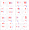 |
Fig. B.1 Abundance ratios [Mg∕Fe],[Si∕Fe], [Ca/Fe],[Ti/Fe] I,and [Ti/Fe] II from this work as a function of temperature. Blue squares are for UVES stars and red circles for GIRAFFE stars. Error bars from Table C.3 are those referred to GIRAFFE (except for [Ti/Fe] II). |
Appendix C Tables of sensitivity and internal errors
Sensitivities to errors in the atmospheric parameters (UVES).
Sensitivities to errors in the atmospheric parameters (GIRAFFE).
Errors in abundances due to errors in atmospheric parameters and in the EWs.
Appendix D Comparison with the GES, APOGEE, and GALAH surveys
Comparison with GES (232 stars, six GCs), GALAH (158 stars, eight GCs), and APOGEE (373 stars, 15 GCs).
 |
Fig. D.1 Comparison of [Fe/H],[Mg/Fe],[Si/Fe], [Ca/Fe],[Ti/Fe] I,and [Ti/Fe] II ratios from the present work (left panels) and the GES survey (right panels). Filled points for GES are stars with UVES U580 spectra. |
 |
Fig. D.2 Comparison of metallicity [Fe/H] and [Mg/Fe],[Si/Fe], [Ca/Fe],[Ti/Fe] I,and [Ti/Fe] II ratios from the present work (left panels) and the GALAH survey (right panels). |
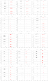 |
Fig. D.3 Comparison of metallicity [Fe/H] and [Mg∕Fe],[Si∕Fe], [Ca∕Fe],[Ti∕Fe] I,and [Ti/Fe] II ratios from this work (left panels) and the APOGEE survey (right panels). |
We adopt the usual spectroscopic notation, i.e. [X]= log(X)star-log(X)⊙ for any abundance quantity X, and log ε(X) = log(NX/NH) + 12.0 for absolute number density abundances.
With these criteria all the 15 stars in common for NGC 3201 are eliminated and we are left with only eight GCs.
The in situ origin for NGC 6388 is also corroborated by Fe-peak elements (Carretta & Bragaglia 2022) in a large number of stars, not only by the α-elements.
Apart from NGC 3201, where the correlation, with p=0.076, is formally not statistically significant.
All Tables
All Figures
|
Fig. 1 Fractions of stars with primordial (P, red circles), intermediate (I, blue circles), and extreme (E, green circles) composition in our programme GCs, superimposed to a reference sample of unpolluted field stars from Carretta (2013, : grey open triangles). |
| In the text | |
|
Fig. 2 Average abundance ratios [Mg/Fe], [Si/Fe], [Ca/Fe], [Ti/Fe] I as a function of metallicity [Fe/H], with the 1σ spread represented as error bars. Filled symbols are for the 16 GCs of the present work, empty symbols indicate GCs from previous individual studies. Red and blue colours are for in situ and ex situ GCs, respectively. Grey points are field stars from Gratton et al. (2003). |
| In the text | |
|
Fig. 3 Differences of the average [Si/Fe] abundance from this work (extended sample) and APOGEE (from Horta et al. 2020) for 20 GCs in common. Symbols are as in Fig. 2. |
| In the text | |
|
Fig. 4 Abundance ratios [Mg/Fe], [Si/Fe], and [Ca/Fe] as a function of the orbital energy of the GCs, from Savino, & Posti (2019). Red and blue symbols are for GCs formed in situ and associated with Gaia-Enceladus. Filled and empty circles refer to the present and previous works, respectively. In each panel, the abundance level of NGC 288 is indicated by the vertical line. |
| In the text | |
|
Fig. 5 Average abundance ratios [Mg/Fe] and [Si/Fe] for GCs in our extended sample, using only the unpolluted P fraction (left panel), the polluted component with intermediate I and extreme E composition (middle and right panel, respectively) in each GC. The horizontal lines trace by eye the upper envelope of abundances in the left panel and are reproduced in the other two panels. |
| In the text | |
|
Fig. 6 Results of the Kolmogorov-Smirnov test on the cumulative distributions of the [Mg/Fe], [Si/Fe], and [Mg/Si] of the P, I, and E components in the 16 programme GCs. In each panel the probability of the K-S test for the comparison P-I and P-E is listed. |
| In the text | |
|
Fig. 7 The Na-Mg anti-correlation in the GCs of our programme sample where the linear regression between Na and Mg is found to be statistically significant (p-value < 0.05). The Pearson’s correlation coefficient and probability are listed in each panel together with a typical error bar. |
| In the text | |
|
Fig. 8 The Si-Na correlation in the GCs of our programme sample where the linear regression is found to be statistically significant. A typical error bar is shown. |
| In the text | |
|
Fig. 9 Diagnostic plot [Ca/Mg] as a function of [Ca/H] for the stars of 16 GCs in the present study (empty grey points). In the left panel, green filled circles are stars in NGC 2808 from Carretta 2015, in the middle and right panels, red and blue filled circles are stars in NGC 7078 and NGC 6752, respectively, from the present work. |
| In the text | |
|
Fig. 10 Detection of Ca excesses in NGC 6752 (left panels) and NGC 7078 (right panels). In the upper left panels GC stars (blue squares) are superimposed to field stars (with typical error of 0.08 dex), and all abundances are linearised in the upper right panels (see text). Generalised histograms of the [Ca/H] values for field (grey area) and GC stars (blue area) are in the lower left panels and the cumulative distributions are shown in the lower right panels, together with the probability of the two-tailed K-S test. |
| In the text | |
|
Fig. 11 Ratios [α/Fe] (average of [Si/Fe], [Ca/Fe], [Ti/Fe]) as a function of metallicity. Grey circles are field stars from Gratton et al. (2003). Blue and red filled circles are accreted and in situ GCs in our extended sample. |
| In the text | |
|
Fig. 12 Fraction of stars with excesses of Ca in 8 GCs from the census in Carretta & Bragaglia (2021, red points)) as a function of a linear combination of GC mass (Baumgardt et al. 2019) and metallicity (Harris 2010). Blue points are for NGC 7078 and NGC 6752 from the present work. A linear fit is given by the solid line, with the Pearson’s correlation coefficient and the two-tailed probability listed in the panel. |
| In the text | |
|
Fig. B.1 Abundance ratios [Mg∕Fe],[Si∕Fe], [Ca/Fe],[Ti/Fe] I,and [Ti/Fe] II from this work as a function of temperature. Blue squares are for UVES stars and red circles for GIRAFFE stars. Error bars from Table C.3 are those referred to GIRAFFE (except for [Ti/Fe] II). |
| In the text | |
|
Fig. D.1 Comparison of [Fe/H],[Mg/Fe],[Si/Fe], [Ca/Fe],[Ti/Fe] I,and [Ti/Fe] II ratios from the present work (left panels) and the GES survey (right panels). Filled points for GES are stars with UVES U580 spectra. |
| In the text | |
|
Fig. D.2 Comparison of metallicity [Fe/H] and [Mg/Fe],[Si/Fe], [Ca/Fe],[Ti/Fe] I,and [Ti/Fe] II ratios from the present work (left panels) and the GALAH survey (right panels). |
| In the text | |
|
Fig. D.3 Comparison of metallicity [Fe/H] and [Mg∕Fe],[Si∕Fe], [Ca∕Fe],[Ti∕Fe] I,and [Ti/Fe] II ratios from this work (left panels) and the APOGEE survey (right panels). |
| In the text | |
Current usage metrics show cumulative count of Article Views (full-text article views including HTML views, PDF and ePub downloads, according to the available data) and Abstracts Views on Vision4Press platform.
Data correspond to usage on the plateform after 2015. The current usage metrics is available 48-96 hours after online publication and is updated daily on week days.
Initial download of the metrics may take a while.