| Issue |
A&A
Volume 707, March 2026
|
|
|---|---|---|
| Article Number | A351 | |
| Number of page(s) | 15 | |
| Section | Planets, planetary systems, and small bodies | |
| DOI | https://doi.org/10.1051/0004-6361/202558500 | |
| Published online | 20 March 2026 | |
How hard is dust in debris disks?
Astrophysikalisches Institut und Universitäts-Sternwarte, Friedrich-Schiller-Universität Jena, Schillergäßchen 2–3, 07745 Jena, Germany
★ Corresponding author: This email address is being protected from spambots. You need JavaScript enabled to view it.
Received:
10
December
2025
Accepted:
9
February
2026
Abstract
The observational appearance of debris disks is largely controlled by collisional grinding of their dust grains. However, the mechanical strength of dust at sizes in the micrometer to millimeter range is poorly known. Recent studies suggest that dust particles in the Solar System might have a higher critical fragmentation energy, Q*D, value than previously anticipated, while another recent study considered the Fomalhaut debris disk and found lower Q*D values to provide better fits to the data. In order to constrain the mechanical strength of dust, we investigate the collisional evolution of debris disks with Q*D prescriptions differing by about three orders of magnitude. We find that, above a certain threshold Q*D value, the disk’s collisional evolution is dominated by rebounding – rather than disruptive or cratering – collisions. Rebounding (also known as bouncing) collisions are those in which both impactors survive, being only slightly eroded and producing fragments that only carry a minor fraction of their mass. We show that disks dominated by rebounding collisions would have brightness profiles increasing outward outside the parent belt. Since such profiles are not observed, this places an upper limit on how hard the debris dust is allowed to be in order not to violate the observations. We derived an approximate analytic expression for this limit, Q*D ≈ (1/8)vK2(r) for grains close to the radiation pressure blowout size, where vK in the Keplerian circular speed at a distance r from the star. This implies Q*D ≲ 109…10 erg g−1 for micrometer-sized grains in typical debris disks. Even though rebounding collisions are not expected to affect debris disk evolution significantly, we emphasize that these collisions are actually much more frequent than disruptive and cratering ones in all debris disks.
Key words: methods: numerical / interplanetary medium / zodiacal dust / circumstellar matter / infrared: planetary systems
© The Authors 2026
 Open Access article, published by EDP Sciences, under the terms of the Creative Commons Attribution License (https://creativecommons.org/licenses/by/4.0), which permits unrestricted use, distribution, and reproduction in any medium, provided the original work is properly cited.
This article is published in open access under the Subscribe to Open model. This email address is being protected from spambots. You need JavaScript enabled to view it. to support open access publication.
1 Introduction
Debris disks encircling a sizable fraction of stars are collections of solid bodies spanning a broad size range, perhaps from dwarf planets as large as ∼1000 km down to micrometer-sized dust (see, e.g. Wyatt 2008; Krivov 2010; Matthews et al. 2014; Wyatt 2020; Pearce 2026, for reviews). However, what is only observed directly is thermal emission of, or stellar light scattered by, dust. Thus, to interpret debris disk observations, one needs to understand the production and sustainment of dust in those disks.
As the very name “debris disk” readily suggests, the key process is destructive collisions. The cascade of collisions grinds larger bodies into ever-smaller ones, down to dust grains. How these collisions exactly work at dust sizes, and thus how the disks appear in observations, depends crucially on the relative velocities of disk particles and their tensile strength. While the former can be estimated, for example from the vertical thickness of the disk (e.g., Matrà et al. 2019; Zawadzki et al. 2026), little is known about the latter. Laboratory impact experiments at the (relatively high) velocities and (relatively small) sizes in question (e.g., Fujiwara et al. 1977; Davis & Ryan 1990; Housen & Holsapple 1999; Nakamura et al. 2015; Landeck 2023; Horikawa et al. 2025) are challenging, and numerical simulations (e.g., Benz & Asphaug 1999; Leinhardt & Stewart 2012, and references therein) do not necessarily yield reliable results either. Both are hampered by the poor knowledge of the material composition of debris dust grains and their morphology (e.g., possible microporosity).
Recent studies suggest that debris dust could be more difficult to destroy than is usually assumed. Rigley & Wyatt (2022) and, more recently, Pokorny et al. (2024) fit zodiacal cloud observations in the Solar System with their collisional and dynamical models to conclude that interplanetary dust in the Solar System must be two to three orders of magnitude more resistant to collisions than previously thought. Sommer et al. (2025), in contrast, find that weaker dust works best to explain the extended sheet of warm dust discovered by JWST in the Fomalhaut system, interior to the main disk (Gáspár et al. 2023).
A standard quantity to characterize the collisional strength of solids is their critical fragmentation energy,  , which is the minimum impact energy per unit mass required to disrupt a body. The idea of this paper is to explore several
  models, including a commonly used model to characterize monolithic grains (Krivov et al. 2018), an alternative stronger model presented in Rigley & Wyatt (2022), and a weak one extrapolated from Sommer et al. (2025). For each
  model, we ran a collisional code to determine the resulting size and radial distributions of dust in a typical disk. We then simulated typical observables, such as spectral energy distributions (SEDs) and radial profiles of brightness, for these models. The goal is to see which
  models make sense and which clearly contradict the observations.
An additional focus of this work is collisional outcomes. If, for instance, the dust is so strong that the typical impact energy is not sufficient to destroy the colliders of some size, it does not necessarily mean that collisions do nothing. Milder outcomes, such as cratering of one or both colliders, bouncing, or even sticking and growth, might still be possible. Our collisional modeling does include a realistic description of all these collisional outcomes. Therefore, in this study, we also explore which types of collisions are important and how they may affect the resulting distributions of dust and the observational appearance of debris disks.
In Section 2, we describe the  models compared in this work. In Section 3, we characterize the possible collisional outcomes we consider, and in Section 4, we describe our collisional code and simulation setup. We present the results in Section 5, discuss them in Section 6, and draw our conclusions in Section 7.
2 Critical fragmentation energy
2.1 General prescription
The outcomes of collisions between the objects sensitively depend on the critical fragmentation energy, which is defined as the minimum impact energy needed to disrupt the body, per unit mass. It depends on the object radius s and the relative (or impact, or collisional) velocity vrel. Smaller bodies are kept together by molecular forces (“strength regime”), whereas larger objects are bound by gravity (“gravity regime”). Accordingly, a standard prescription is the sum of two power laws, one for each regime (Benz & Asphaug 1999):
 (1)
(1)
where coefficients As and Ag depend on the relative speed vrel:
![Mathematical equation: $Q_{\rm{D}}^* = \left[ {A_{\rm{s}}^0{{\left( {{s \over {1{\rm{cm}}}}} \right)}^{{b_{\rm{s}}}}} + A_{\rm{g}}^0{{\left( {{s \over {1{\rm{cm}}}}} \right)}^{{b_{\rm{g}}}}}} \right]{\left( {{{{v_{{\rm{rel}}}}} \over {{v_0}}}} \right)^{{b_{\rm{v}}}}}.$](/articles/aa/full_html/2026/03/aa58500-25/aa58500-25-eq13.png) (2)
(2)
In what follows, we set v0 = 3 km s−1 and bv = 0.5, following Stewart & Leinhardt (2009).
2.2 Typical relative velocities in debris disks
The typical collisional velocities can be inferred from the measured geometric vertical thickness of the disks at (sub)millimeter wavelengths, assuming equipartition of energy (see Jankovic et al. 2024, however). For instance, Terrill et al. (2023) analyzed 16 highly inclined debris disks observed by ALMA. They found a wide range of vertical aspect ratios, h, ranging from 0.020±0.002 (AU Mic) to 0.20±0.03 (HD 110058). The average value for disks with a moderate fractional width is h ∼ 0.03 (for wide disks, it appears to be somewhat higher, ∼0.05). Similarly, the REASONS survey of 74 disks (Matrà et al. 2025) derived aspect ratios in the range from ∼0.01 to 0.3 for a subset of disks for which the vertical thickness could be constrained. Finally, for a set of 13 of the most highly inclined targets observed with ALMA in the ARKS program with the highest resolution achieved today (Marino et al. 2026), the half-width at half-maximum (HWHM) vertical aspect ratios were found to lie in the range 0.0026 ≤ h ≤ 0.193, with a median best-fit value of h = 0.021 (Zawadzki et al. 2026). Assuming roughly h ∼ 0.03 to be a typical value, Eq. (13) of Zawadzki et al. (2026) then gives the typical relative velocity in a disk, assuming equipartition between out-of-plane and in-plane velocities:
 (3)
(3)
where vK is the circular Keplerian speed at the radius of the disk. For our reference disk with a radius of 100 au around a solar-type star, we get vK = 3 km s−1 and vrel ≈ 300 m s−1.
2.3 Traditional model for 
As a reference case (hereafter called “Reference model”), we used a  prescription appropriate for “monolithic,” collision-ally strong planetesimals taken from Krivov et al. (2018, their Eq. (1)):
  ,
,  , bs = 0.37, and bg = 1.38. This prescription is essentially based on the smooth particle hydrodynamics (SPH) simulations by Benz & Asphaug (1999) for basalt
  ,
,  , bs = −0.38, and bg = 1.36) and ice
  ,
,  , bs = −0.39, and bg = 1.26), complemented with the velocity dependence taken from Stewart & Leinhardt (2009). It is also close to results by Jutzi et al. (2010) for basalt, which are
  ,
,  , bs = −0.38, and bg = 1.36.
2.4 Zodi-based model for 
As an alternative case, we defined the “Zodi model.” It is based on the  constraints from Rigley & Wyatt (2022). They fit zodiacal cloud observables with their collisional and dynamical model and found As = 2.0 × 10⁷ erg g−1 and bs = 0.90 (see their Sections 4.2, 6.5 and Fig. 25).
Note that they give As rather than  . To compute the latter, we roughly estimated the typical collisional speeds in their zodi modeling. Their Fig. 14 gives a distribution of mass input into the dust production in terms of pericentric distance q and eccentricity e. To get a rough idea of the collisional speed, we considered two intersecting orbits with the same q and e. The relative velocity at the intersection points is maximum when the two orbits are apsidally anti-aligned, in which case (Costa et al. 2024, their Eq. (A10))
 (4)
(4)
The highest mass input in the model of Rigley & Wyatt (2022) occurs in a stripe on the (q, e)-plane that roughly corresponds to aphelion distances of 4…5 au. This stripe extends from q ≈ 4 au and e ≈ 0 to q ≈ 0.5 au and e ≈ 0.9, with higher values≈ toward lower perihelia (and higher eccentricities). Equation (4) gives a broad range of relative velocities from ≈3 km s−1 to ≈130 km s−1 – again, with preference toward higher values. As a rough proxy for the entire cloud, we took vrel ≈ 30 km s−1. This gives  .
.
Another model comes from Pokorny et al. (2024). They did a similar analysis for the zodiacal cloud and found As = (5.0 ± 4.0) × 109 erg g−1 and bs = −0.24. Assuming, again, vrel ≈ 30 km s−1 to be typical of the zodiacal cloud, this translates to  . However, for simplicity, we will only consider one Zodi-based model and do not investigate this model further.
2.5 Fomalhaut-based model for 
Our third model is the “Fomalhaut” one. It is inspired by Sommer et al. (2025), who investigated the Fomalhaut debris disk and determined a best fit for the  value of 32 µm-sized particles to be
  . That best fit also includes a
  slope of bs = 0.15 and a maximum value of bs,max = −0.45, but the authors do not place high confidence in this value. This steepness is much closer to our Reference model than to the Zodi model. So, to keep things simple, we will extrapolate their result using the slope of the Reference model. While Sommer et al. (2025) report average collisional velocities of 100 m s−1, we scaled their result to v0 = 3 km s−1 to calculate
  .
.
We also note that Rigley & Wyatt (2022) and Sommer et al. (2025) assume a material composition and density different from ours (astrosilicate, 3.3 g cm−3, see Section 4.2). We ignored these differences for two reasons. First, we wished to clearly see the role of changing the  , and not several parameters simultaneously. Second, the expected corrections would only be minor, compared to the other uncertainties involved.
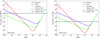 |
Fig. 1 Chosen |


Summary of simulation parameters used.
2.6 Summary of  models
For simulations in this paper, we thus considered three models: Reference, Zodi, and Fomalhaut ones, as defined above. To the latter two, we added the term for the gravity regime with the same parameters  and bg = 1.38 as in the Reference model.
The parameters of all three models are collected in Table 1. The models are depicted in Fig. 1 for different impact speeds of 300 m s−1 (left) and 30 m s−1 (right), corresponding to eccentricity dispersion of 0.1 and 0.01, respectively. Additionally, the model from Pokorny et al. (2024) is shown for comparison. It is seen that dust (i.e., particles up to ∼1 mm in size) is the weakest in the Fomalhaut model, harder to disrupt in the Reference one, and the strongest in the Zodi model. For example, in the Zodi model, the smallest (µm-sized) dust grains are 20–30 times harder than in the Reference one.
Overplotted with horizontal lines is the collisional disruption threshold of  for collisions of two equal-sized particles, estimated as
  (see Eq. (5.2) in Krivov et al. 2005). It shows at which sizes the particles are expected to undergo disruptive collisions and, conversely, which grains are likely to remain essentially “indestructible,” being subject to cratering or rebounding collisions only. Consider, for instance, the left panel of Fig. 1 for 300 m s−1. We see that in the Fomalhaut model, the material is prone to catastrophic collisions at all sizes, and in the Reference one all grains larger than ≈10 µm can be shattered. In contrast, in the Zodi model, grains smaller than hundreds of µm should become indestructible.
3 Collisional outcomes
Once  and vrel are known, the outcome of a collision between two arbitrary objects, the projectile of mass mp and the target of mass mt (such that mp ≤ mt) is to be determined. The impact energy sets the individual fate of either collider according to the following algorithm (Löhne 2015).
First, it is checked whether half the impact energy suffices to disrupt the projectile, i.e., whether  . If this is the case, the projectile mass is added to the fragment mass budget and the remaining energy of the projectile’s half is assumed to be imparted on the target. Otherwise, the projectile is assumed to be cratered but rebounding from the target or sticking to it – depending on whether the impact velocity is below or above a threshold of 10 m/s. Owing to this low threshold, sticking collisions do not occur in our simulations considered here.
Second, the remaining energy – at least half of the total impact energy – can either disrupt or crater the target and lead to the dispersal of either the total mass or part of it, respectively. This “equipartition” of impact energy between the two colliders can only be assumed if their material strengths are comparable. What comes out is either the sum of the two remnants (which can be zero if both are dispersed) or two individual remnants, and the joint fragment mass (which can be as large as the sum of both colliders).
Hence, there are four different combinations for the mass of the remnant(s), mrem, and that of the fragments, mfrag (see Fig. 2). For disruptive (or destructive, or shattering, or catastrophic) collisions, in which both colliders are destroyed, we have
 (5)
(5)
Cratering (or erosive) collisions are such that the target gets cratered, while the projectile is destroyed:
 (6)
(6)
 (7)
(7)
Rebounding (or bouncing, or “double-cratering”) collisions imply that both impactors survive, only undergoing some erosion, and bounce off each other:
 (8)
(8)
 (9)
(9)
 (10)
(10)
Finally, sticking (or agglomerating) collisions are those in which both colliders essentially merge, with only a minor fraction of their mass going into fragments; these are characterized by
 (11)
(11)
 (12)
(12)
 |
Fig. 2 Schematic of the four possible collisional outcomes, Eqs. (5)–(12). The “projectile” particle (the less massive of the two colliders, marked with “p” and shown in red), and the “target” one (the more massive one, “t,” in blue) collide to produce one or two remnants (“rem” or “rem, p” and “rem, t,” each having the color of its progenitor particle) and a cloud of fragments that may originate from both colliders (“frag,” shown in black). |
4 Collisional simulations
4.1 The ACE code
To model the collisional evolution of the disks, we used the collisional code ACE (“Analysis of Collisional Evolution”; Krivov et al. 2005, 2006, 2013; Löhne et al. 2008, 2012, 2017; Sende & Löhne 2019). The code assumes a certain central star and a planetesimal disk of certain size, mass, excitation, and other parameters such as mechanical and optical properties of disk particles (including Q∗D) as input. The code simulates the collisional evolution of the debris disk by solving a kinetic Boltzmann-Smoluchowski equation in a 4-dimensional grid which comprises masses of solids, periastron distances, eccentricities, and longitudes of the periastron as phase space variables. The vertical dimension (defined by the orbital inclination and the longitude of the ascending node) is averaged over. Collisional outcomes are treated as described in Section 3. For every instant of time, the distribution of the phase variables is converted into the coupled radial and size distributions of solids – from planetesimals to dust.
An auxiliary program, called PHSimage, takes the ACE output as input and computes the observables (both in thermal emission of dust and scattered stellar light). Specifically, in the subsequent sections we computed the time evolution of disk brightness, SEDs, as well as brightness profiles of our model disks at selected wavelengths from near-infrared to millimeter.
4.2 Simulation setup
We performed a set of three runs, corresponding to  prescriptions listed in Table 1. For all runs, we used a solar-mass star M∗ = M⊙ with solar luminosity L∗ = L⊙. It was surrounded by an initially narrow and thin debris disk between 95 au and 105 au with a small semi-opening angle ϵ = 0.05 rad populated initially by particles in the size range 1 µm ≤ s ≤ 200 km, whose orbits had eccentricities uniformly distributed over 0 ≤ e ≤ 0.1. The initial size distribution was given by dN ∝ s−qds with q = (21 + bs)/(6 + bs), where bs is the exponent for the strength-regime part of the
  prescription (O’Brien & Greenberg 2003). The initial disk mass M0 in all runs was set to M0 = 100 M⊕, although the runs were scaled to arrive at the same dust mass at the given instant of time (see Section 5.1). The longitude of the periapsis was assumed to be distributed uniformly, so that the disk was rotationally symmetric at all times. We disregarded collisions involving particles on unbound orbits, stellar wind effects, and Poynting–Robertson drag and did not include gas in the debris disk. Gravitational interactions between disk solids were not modeled either. We included stellar radiation pressure, assuming astrosilicate particles (Draine 2003) with a density of ρdust = 3.3 g cm−3. To this end, we used the Mie theory (Bohren & Huffman 1983) to compute the radiation pressure-to-gravity ratio, β, as a function of grain radius s (Burns et al. 1979). For this material and the Sun-like central star, the blowout size is sblow = s(β = 0.5) = 0.5 µm.
5 Results
5.1 Long-term evolution
Fig. 3 (dashed lines) shows the typical temporal evolution of dust in the simulated disks. Although the initial disk mass was set to the same value, different tensile strengths of material in our runs cause their disks to lose mass at different rates. As a result, the disks contain different amounts of dust, and are unequally bright, at any time instant of interest. Therefore, for a better comparison of the runs, it is natural to rescale them to have the same amount of dust (or brightness) at some moment of their evolution.
Such a rescaling is easily done without rerunning the collisional code, by applying the following rule (Löhne et al. 2008; Krivov et al. 2008). In a collisionally dominated debris disk in a quasi-steady state with initial disk mass M0 and disk age t, for any quantity F that is directly proportional to the disk mass in any size interval in which particles are created and destroyed by collisions (e.g., dust mass), there is a relation
 (13)
(13)
valid for any real number x > 0. However, in any size interval occupied by unbound grains, which are not lost in collisions but get blown out by radiation pressure on (short) dynamical timescales, the following relation holds instead (see Appendix A):
 (14)
(14)
Specifically, we chose to rescale the Fomalhaut and the Zodi runs to have the same dust mass (in particles s < 1 mm) at an arbitrary time instant (which we took to be 100 Myr) as the Reference run. Applying Eqs. (13) and (14) to the Zodi and Fomalhaut runs, we found x = 0.0032 and x = 5.0, respectively. The resulting curves are depicted in Fig. 3 with solid lines. In the rest of the paper, we analyze these rescaled runs.
The dust mass starts to decrease as soon as the collisional lifetime of the weakest particles, called τb in Löhne et al. (2008), is reached. In all three runs, this happens pretty early, in ∼104– 106 yr. The subsequent loss of dust mass occurs roughly as ∝ t−0.5, broadly consistent with the theoretical predictions (Löhne et al. 2008) and statistics of debris disks of different ages (e.g., Zuckerman & Becklin 1993; Habing et al. 1999, 2001; Spangler et al. 2001; Greaves & Wyatt 2003; Rieke et al. 2005; Moór et al. 2006, Moór et al. 2015; Eiroa et al. 2013; Chen et al. 2014; Holland et al. 2017; Sibthorpe et al. 2018). Since the falloff of dust mass is similar in all three models, it is not possible to constrain the mechanical strength of debris dust from the analysis of the long-term evolution.
We have also computed the time evolution of disk brightness at two wavelengths, 1 mm and 1 µm. These choices correspond to observations with instruments such as SPHERE (Beuzit et al. 2019) or GPI (Macintosh et al. 2014) and ALMA (Wootten & Thompson 2009), respectively. The 1 µm profiles are almost entirely made up of scattered stellar light and the 1 mm ones represent thermal radiation of the dust itself. As the stellar spectrum, we took the solar photospheric model from Woods et al. (2009), and the scattered light was computed with a Mie phase function (Bohren & Huffman 1983).
The results are shown in Fig. 4. Not surprisingly, the millimeter flux behaves in a similar way to the dust mass. Interestingly, though, the same applies to the total intensity in scattered light. Note that for the Zodi run, the decay of the 1 µm flux sets in later, at several Myr; this is caused by the peculiar behavior of µm-sized grains discussed in detail in Section 5.3, and by the longer time they need to find a steady state. However, the debris disk samples used in statistical studies cover systems older than ∼10 Myr. Thus the conclusion remains the same: one cannot distinguish between our models based on the statistics of disk fluxes at different ages.
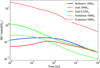 |
Fig. 3 Dust mass evolution for the three runs. Dashed lines depict the original (unscaled) and solid lines the scaled versions of the runs. Only one curve is shown for the Reference run as the scaled and unscaled versions are equivalent here. |
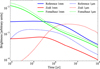 |
Fig. 4 Time evolution of disk brightness in all three runs at 1 µm (dashed lines) and 1 mm (solid lines). |
5.2 Size distribution
As in our previous papers (e.g. Krivov et al. 2006; Krivov et al. 2018), size distributions in this work are given as cross-section density distributions per size decade. That is, we plot the total cross-section area of the disk objects per unit log size bin per unit disk volume.
The size distributions of the three runs at 100 au are plotted in Fig. 5. All three size distributions are typical of collision-ally evolved disks. The cross-section density peaks somewhat above the blowout limit: around 7 µm for the Zodi run, at 5 µm for the Reference run, and at 0.5 µm for the Fomalhaut run (see Pawellek & Krivov 2015, for a discussion of how the peak position is related to the blowout limit). The size distribution to the left of the blowout limit is dominated by dust on hyperbolic orbits. To the right of the peak, the slope of the distribution is set by the  prescription used (O’Brien & Greenberg 2003), with a characteristic minimum in the transition region between the material strength regime and the gravity regime (at ∼10…100 m). At the very right lie the planetesimals that have not reached their collisional lifetime yet, which therefore retain their initial (primordial) distribution. Ripples seen above the blowout limit and above the transition to gravity-dominated regimes at 107–108 µm, especially for the Fomalhaut run, are a known phenomenon (e.g., Campo Bagatin et al. 1994; Wyatt et al. 2011) and are not discussed further.
As a side remark, the above analysis also confirms that the same dust mass at a given age can result from a population of planetesimals of a lower initial mass if  is steeper, as expected – potentially mitigating the “debris disk mass problem” (Krivov et al. 2018; Krivov & Wyatt 2021). For instance, our Zodi run with just 0.32 M⊕ in planetesimals sustains the same amount of dust at 100 Myr as the Reference run disk with the total mass of 100 M⊕ (cf. blue and red solid lines in Fig. 3). It is highly questionable, however, whether a nontraditional
  model such as that of the Zodi run is a solution to this problem. The more so, since it is not clear yet whether simulation results for alternative models are compatible with other debris disk observables, such as radial profiles of brightness at different wavelengths. This is considered in the subsequent sections.
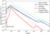 |
Fig. 5 Size distribution at 100 au in the three runs in the initial state (thin lines) and at T = 100 Myr (thick lines). |
5.3 Spatial distribution
Next, we look at the optical depth profiles of the simulated debris disks (Fig. 6). For an idealized disk, the normal geometrical optical depth τ should decay at greater distances from the star as (Strubbe & Chiang 2006; Krivov 2010)
 (15)
(15)
While the optical depth profiles in the Reference and Fomalhaut runs do converge to this idealized one, the profile in the Zodi run differs dramatically. In this case, the optical depth increases farther out from the star, which is totally unexpected and needs to be understood. In addition, the profile is not quite smooth, exhibiting, for instance, some dips at ≈ 160 au and ≈ 240 au. This behavior arises from the discrete phase space grid of the numerical simulation.
To find a physical mechanism behind the increasing optical depth profile in the Zodi run, we first looked at the size distribution of dust at different locations, both in the parent ring and exterior to it. The left panel of Figure 7 shows the size distribution for s < 10 µm in all three runs at 100 au, 200 au, and 300 au. For the Reference and Fomalhaut runs, the 100 au distribution extends across the entire size range, the 200 au distribution has a significant cross-section density between somewhat below the blowout size and ≈2 µm, and the 300 au distribution between the minimum size and ≈1 µm. However, the Zodi run is very different. The 100 au distribution has a broad peak at s ≈ 5 µm, and the 200 au and 300 au distributions feature very sharp peaks at 0.9 µm and 0.6 µm, respectively. This suggests that in the Zodi run, each radial location in the outer disk is preferentially populated by grains of specific sizes. While size sorting is a known phenomenon in debris disks (Strubbe & Chiang 2006; Thébault & Wu 2008; Thebault et al. 2014), the effect is much more pronounced in the Zodi run than in the Reference and Fomalhaut runs.
Next, we checked the average orbital eccentricity of different-sized dust grains in the same runs and at the same three distances as before. The results are shown in the right panel of Fig. 7. We see that in the Zodi run, the size distributions in the outer disk (at 200 au and 300 au) peak at the grain sizes at which the average eccentricity reaches its minimum. This implies that specific regions in the outer disk exist where particles of certain sizes accumulate on nearly circular orbits.
Trying to explain why in the Zodi run small grains concentrate in nearly circular orbits on the outer disk, we made additional test runs with different combinations of collisional outcomes described in Section 3. The results are described in Appendix B. We found that excluding rebounding collisions (Eqs. (8)–(10)) changes the evolution dramatically (see Appendix B). This is illustrated by Fig. B.1 (radial profiles of optical depth), Fig. B.2 (size distribution), and Fig. B.3 (average eccentricity of grains of different sizes). Excluding cratering collisions in addition to rebounding collisions brought about results that were almost indistinguishable from those with just the rebounding collisions removed. No runs were performed without sticking collisions, as they occur too rarely to make a difference.
Accordingly, next we focus on how rebounding collisions in the Zodi run circularize orbits of dust grains of specific sizes. Analysis of the simulation bins uncovered the following picture (Fig. 8):
– Collisions in the parent ring at R = 100 au generate dust. Grains with a certain size s and β = β(s) are sent by radiation pressure in eccentric orbits with semimajor axes and eccentricities (Burns et al. 1979)
 (16)
(16)
respectively. The pericenter of these orbits lies in the parent ring at rΠ = R, and apocenter is at rA = R/(1 − 2β). These grains form well-known halos exterior to the parent belt.
– Around the apocenter, rebounding collisions between those grains and highly eccentric particles with pericenters in the main belt produce yet smaller dust debris. Again, radiation pressure sends these to new orbits with semi-major axes a′′ and eccentricities e′′, depending on their β-ratio. Since the release point of those secondary debris is at the apoc-enter, there exist some sizes s′ (and β′) such that the new debris gets on circular orbits with a′′ = rA and e′′ = 0. The enhancement of density (or optical depth) at distance r caused by grains on circular orbits is a simple geometrical effect (see, e.g. Haug 1958).
Next, we consider a certain distance r in the outer disk (e.g., one of the distances at which an enhanced optical depth is seen in Fig. 6). It is easy to derive both the β-ratio of the “primary” ejecta from the parent ring with apocenters at distance r,
 (17)
(17)
and that of the “secondary” debris arising from rebounding collisions and placed into circular orbits or radius r,
 (18)
(18)
Next, we make simple numerical estimates. At r = 200 au, we obtain β = 0.25 and β′ = 0.50, which translate to sizes s = 0.9 µm and s′ = 0.5 µm. At r = 300 au, we get β = 0.33 and β′ = 0.67, which correspond to sizes s = 0.7 µm and s′ = 0.4 µm. The sizes s′ deviate somewhat from the positions of the eccentricity minima seen in Fig. 7, which are 0.9 µm and 0.6 µm, respectively. Further investigation revealed that while the size-dependent radial location of the circularized dust does not perfectly match the predictions of Eq. (18) at 100 Myr, it does at beginning of the collisional evolution. To demonstrate this, in Fig. 9 the positions of the peaks of the size distributions of the Zodi run versus stellocentric distance are plotted at system ages of 0.01 Myr, 0.1 Myr, and 100 Myr. The expected grain sizes from Eq. (18) are overplotted for comparison. It is evident that, at 0.01 Myr, the Zodi run matches Eq. (18) reasonably well, but starts to deviate from it quickly, with even the 0.1 Myr distribution being very different from it. This suggests that the circular dust orbits in the Zodi run do appear at the positions predicted by Eq. (18) and later “migrate” outwards. Analyzing the simulation bins, we conclude that expansion of the circular dust orbits is caused by a cascade of rebounding collisions which gradually erode the grains, reducing their sizes, and shift them to greater radii. Further details and plots illustrating the circularization of dust orbits in the Zodi run are given in Appendix C.
The question arises why we do not see such circular orbits in the Reference and Fomalhaut runs. In all three runs, dust particles born in the main belt are placed in orbits with high apocenters by radiation pressure. However, only in the Zodi run, rebounding collisions dominate, which reduce particle sizes more gently than disruptive collisions would do, producing grains with “right” sizes (Eq. (18)) to get in circular orbits. In the Reference and Fomalhaut runs, however, these particles get destroyed via disruptive collisions with high-eccentricity grains stemming from the main belt. The fragments of these collisions are too small to be placed by radiation pressure in circular orbits. Instead, they typically get in hyperbolic orbits and are blown out of the system. If any particles on circular orbits are produced, they are quickly destroyed by subsequent collisions.
In summary, we found that a disk of hard dust, represented by our Zodi run, contains a large amount of small dust particles in circular orbits at large stellocentric distances. These are produced by rebounding collisions in the outer disk and, due to their high  value, survive subsequent collisions with other particles. These small dust grains in circular orbits are so numerous that the cross-section density in the outer disk gets larger than in the main belt (see Fig. 7 left). It is this phenomenon that explains the increase of the optical depth with distance seen in Fig. 6.
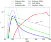 |
Fig. 6 Radial profiles of normal geometrical optical depth in the three runs. An idealized profile (Eq. (15)) and is shown for comparison. Both axes are logarithmic. |
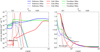 |
Fig. 7 Size distribution of dust grains (left) and average eccentricity of different-sized dust grains (right) in the Reference, Fomalhaut, and Zodi runs at three selected stellocentric distances: 100 au (solid lines), 150 au (dashed), and 200 au (dotted). Note that only dust grains smaller than 10 µm are shown. In both panels, the blowout grain size is marked with a vertical black line. |
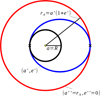 |
Fig. 8 Schematic of the proposed circularization mechanism. Black, the parent belt; blue, a halo grain; red, a secondary debris particle in a circular orbit. |
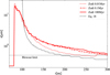 |
Fig. 9 Peak positions of cross-section density distributions of the Zodi run as functions of distance from the star at three different system ages. Overplotted in black is the theoretical curve, Eq. (18). |
5.4 Spectral energy distributions
Our intention in this study is to find out whether one can distinguish between different  models from debris disk observations. The simplest “observable” for a debris disk is its SED. However, the SEDs derived for our three runs turn out to be pretty similar (Fig. 10). This might not be intuitive as the size distributions differ markedly (Fig. 5). In particular, Zodi run’s distribution peaks at a larger particle size than the Reference run’s. Since larger particles at the same distance are colder, we should expect its SED to peak at a longer wavelength. However, Fig. 5 only shows the size distribution at 100 au, whereas the Zodi disk contains many more small particles at larger stellocentric distances. The net effect is that the SEDs are roughly the same. Indeed, most of the Zodi run’s SED originates from high stellocentric distances and not from the main belt. This can be seen in Fig. 10, where the hatched area represents the part of the SED which is generated by the outer disk at r > 150 au. While its contribution can be neglected for the Reference and Fomalhaut runs, it makes up most of the SED for the Zodi run.
To compare the SEDs quantitatively, a useful quantity is Γ, the ratio of the dust belt radius R and its blackbody radius Rbb (Booth et al. 2013; Pawellek et al. 2014; Pawellek & Krivov 2015):
 (19)
(19)
where R = 100 au in our simulations, and the blackbody radius is given by (Backman & Paresce 1993)
 (20)
(20)
with L∗ being the stellar luminosity and Tdust the dust temperature,
 (21)
(21)
which is computed from the peak wavelength λmax of the SED (assuming that thermal emission flux is given in Jy, i.e., is measured per unit frequency).
The thermal emission of all three dust belts peaks at λpeak = 63 µm which, using the above formulae, corresponds to a black body equilibrium temperature of T = 81 K and a blackbody radius of Rbb = 12 au. The resulting Γ = 8.3 is therefore the same for all three runs and thus prevents one from distinguishing between different  prescriptions based on a disk’s SED.
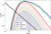 |
Fig. 10 Thermal emission SEDs in the three runs analyzed (colored lines). The hatched regions indicate the portion of the SEDs generated by the part of the disk outside of 150 au. The black line is the stellar photosphere. |
5.5 Radial brightness profiles
While the differences in the optical depth profiles (Fig. 6) are interesting, more promising for our purposes are brightness profiles at different wavelengths. We computed them as explained in Section 5.1. These are shown in Fig. 11 for the three runs after 100 Myr, both in scattered light at 1 µm and in thermal emission at 1 mm.
For the sake of clarity, we only consider here the simplest case of a debris disk with a single, narrow parent belt (see the setup of our simulations, Section 4.2). A significant fraction of the observed disks do belong to this category (Han et al. 2026). We note, however, that disks with a more complex radial structure exist as well. Some appear broad at millimeter wavelengths (e.g. Matrà et al. 2025; Marino et al. 2026), while some others contain multiple parent rings, often both narrow and broad (Han et al. 2026). There are even atypical systems such as HD 131835 (Jankovic et al. 2026) where the millimeter and scattered-light profiles peak at completely different distances from the star. Analysis of such systems is out of the scope of this paper and would require a separate study.
In thermal emission, brightness profiles of debris disks with a single, narrow parent belt are observed to show a pronounced peak around the parent belt, followed by a falloff farther out from the star that often drops quickly to below the noise level (e.g., Marino 2021; Han et al. 2026). In scattered light, a peak nearly at the same position1 as with thermal radiation is seen, followed by a gentle decrease in brightness, often – although not always – approximately as r−3.5 (Thébault & Wu 2008; Thébault et al. 2023; Engler et al. 2025; Milli et al. 2026). Figure 11 readily demonstrates that both Reference and Fomalhaut profiles are fully compatible with these expected brightness profiles. It would be difficult to distinguish between the two models, Reference and Fomalhaut, given numerous and diverse uncertainties, ranging from unknown distributions of dust-producing planetesimals to challenges of finding the phase function that reproduces scattered light data adequately.
While the Reference and Fomalhaut runs yield reasonable results fully compatible with typical debris disk data, the Zodi profiles are completely different. The only similarity of the thermal emission profile with actual data is that it peaks at the parent ring. Exterior to it, the brightness profile is pretty flat. This might seem unexpected given that 1 mm flux is typically generated mostly by dust roughly of the size of 1 mm, and that there is no such dust at distances of 200 au or greater (see Fig. 7). In this case, however, the 1 mm flux is generated by the very small ≈1 µm dust which is abundant at those distances. While its absorption and emission efficiency is very low, Qabs ~ 10−4 using Fig. 6 from Krivov et al. (2008), the amount of small dust is so high that the mm flux in the outer disk stays nearly constant. The scattered-light profile of the Zodi run is pathological as well, and clearly at odds with the actually observed profiles. No traces of the parent ring are visible at all, and the brightness increases outward.
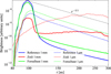 |
Fig. 11 Profiles of disk brightness (per pixel) in the three runs after 100 Myr of evolution, at wavelengths of 1 µm (dashed) and 1 mm (solid lines), using a resolution of 1 au/pixel. |
6 Discussion
6.1 When is dust too hard?
In Sections 5.3 and 5.5, we found that lowering the  value of dust particles below the value of the Reference run does not significantly alter the radial profile of a debris disk, while increasing
  leads to peculiar profiles that are clearly incompatible with observations. This raises a question: When is dust too hard?
From Section 5.3 and the analysis in Appendix C, we know that peculiar radial profiles arise if small particles in the outer disk are placed in circular orbits. This was the case in the Zodi run. And conversely, orbits of small dust grains in the outer disk do not get circularized, if their source – halo particles with pericenter in the main belt and apocenters far away from the star – get destroyed by near-blowout particles created in the main belt. In this case, exemplified by the Reference run, the radial profiles are “normal” and consistent with the observed ones.
This allows us to derive a simple criterion for the absence or presence of dust grains in circular orbits in the outer disk. Analyzing the results of the Reference run, we found that only 10–20% of collisions between the near-blowout particles and the halo ones occur in the main ring, while half of them happen far away from it, closer to the apocenters of the halo grains. To make a rough estimate, we assume that the collisions take place at the apocenters. Further, we assume that small projectiles, which are created at R and are to destroy a particle of size st in an eccentric orbit with apocenter at r, the splinter fragments of which would get in a circular orbit of radius r, have β = 1/2 and so exactly the blowout size sblow. They move away from the star in a parabolic orbit, so that their velocity at the distance r is
 (22)
(22)
where vK(r) is the circular Keplerian speed at a distance r. Finally, we assume that the relative velocity between the target particles in eccentric orbits and projectiles in parabolic ones is approximately equal to the speed of the latter, v.
The maximum critical fragmentation energy  for which the collision will be disruptive is given by (see Eq. (5.3) in Krivov et al. 2005)
 (23)
(23)
or
 (24)
(24)
where mblow and mt are the masses of the blowout-sized bullets in parabolic orbits and the target grains in eccentric orbits, respectively. Equations (23) and (24) are valid for mblow ≪ mt.
We now express st through the distance r. Since grains of size st are the source of grains in circular orbits at the distance r, their β is given by Eq. (17). Assuming that radiation pressure efficiency for particles with st > sblow is unity, β ∝ 1/s, and we write
 (25)
(25)
so that
 (26)
(26)
With the above assumptions and using Eqs. (22) and (26), Eq. (24) takes the form:
 (27)
(27)
For any distance r > R in the outer disk, Eq. (26) gives the size st, and Eq. (27) gives the maximum  that dust grains of that size are allowed to have in order not to send splinters to circular orbits and not to form abnormal radial profiles.
Since the above derivation assumes mblow ≪ mt, the model is no longer valid for r ≫ R. In that case, a general Eq. (5.2) from Krivov et al. (2005) instead of Eq. (5.3) shall be used. For large r, Eq. (26) becomes
 (28)
(28)
and Eq. (27) is replaced by
 (29)
(29)
We make some numerical estimates with Eqs. (26)–(27), which are valid at distances within a few R. As before, we take R = 100 au, v(R) = 3 km s−1, and sblow = 0.5 µm. At r = 2R = 200 au, we get st = 1 µm (close to the exact value 0.9 µm which comes from the actual β(s) dependence that assumes a realistic radiation pressure efficiency) and  . This is larger than
  at 0.9 µm of the Reference run, 7 × 10⁸ erg g−1, and smaller than in the Zodi run, 2 × 10¹⁰ erg g−1. Similarly, at r = 3R = 300 au, the result is st = 0.75 µm and
  . Again, this is larger than
  in the Reference run and smaller than in the Zodi one. At large distances, such as r = 10R = 1000 au, we use Eqs. (28)–(29) to get st ≈ 0.5 µm and
  . These estimates are fully consistent with that fact that circular orbits do appear in the Zodi run, but get destroyed in the Reference run.
The above analysis gives the strength threshold above which small grains in the outer disk are sent into circular orbits. Strictly speaking, this alone may not be sufficient for peculiar brightness profiles to arise. It can happen that circular orbits form, but get swiftly destroyed – by the same near-blowout particles produced in the main ring. To check when this happens, we start again with the relative velocities between the target grains in circular orbits and near-blowout grains impacting them. Within a factor of two, these relative velocities are still given by Eq. (22). Further, particles in circular orbits typically have sizes close to the blowout one (see Section 5.3). Therefore, we now have the case st ≈ sblow, which is described by Eq. (29). We conclude that the criteria for creation and survival of dust grains in circular orbits are almost the same. For ball-park estimates, one can simply use Eqs. (28)–(29).
6.2 Caveats
In our simulations, several physical effects of potential importance were omitted. One of the them is the Poynting-Robertson (PR) effect. The PR effect can often, although not always, be ignored, especially in bright disks that have high optical depth (Wyatt 2005; Kennedy & Piette 2015; Rigley & Wyatt 2020; Sommer et al. 2025). This is because the collisional lifetimes of dust particles are typically much shorter than their PR lifetimes. However, in this work’s Zodi run, collisions are not necessarily catastrophic anymore and, at least in the outer region of the disk, just slightly erode the particles and stochastically change their orbits. As a result, grain lifetimes in disks composed of hard dust may become much longer. Therefore, including PR effect in simulations seems reasonable. Accordingly, we made an additional test run with the same setup as in the Zodi one, but with the PR drag switched on. The differences to the normal Zodi run without PR drag turned out to be only marginal.
Nevertheless, including the PR effect is absolutely necessary for debris disks with low fractional luminosities such as the Solar system’s zodiacal dust cloud. Therefore, we performed one more Zodi run with PR drag included and an initial disk mass set to an arbitrary low value (10−4 M⊕). This run did not reveal the pathological optical depth profile seen in the Zodi run. Instead, the profile turned out to be perfectly consistent with the one typical of transport-dominated disks: τ ∝ r−2.5 exterior to the parent ring and τ ∝ r0 interior to it (Strubbe & Chiang 2006). We conclude that the constraints on  obtained in this paper do not necessarily apply to disks with low optical depths. This might also be part of the explanation why Rigley & Wyatt (2022) found hard dust to fit well the zodiacal cloud data (see also discussion in Section 6.3). Including the PR effect would be required to place constraints on the critical fragmentation energy of dust in such disks. Unfortunately, handling transport processes like PR drag is more expensive computationally than that of pure collisional evolution. Also, the mass scaling (Eq. (13)) is not valid in the presence of transport, which would further hamper the analysis.
Another effect not included in our modeling is collisional damping (Pan & Schlichting 2012). This might become important in realistic disks with hard dust (Jankovic et al. 2024). If so, damping would also affect the vertical velocities, flattening the disks. Such effects cannot be modeled with our collisional code ACE, as it assumes the vertical velocities to be constant and does not resolve the inclination.
6.3 Do rebound-dominated disks exist?
In collisional modeling of debris disks, it is typically assumed that disks are dominated by disruptive collisions (see, e.g., Dohnanyi 1969; Wyatt et al. 1999; Wyatt & Dent 2002, among others). Thébault et al. (2003) and Kobayashi & Tanaka (2010) pointed out that cratering collisions can be even more important in many cases. In this work, we found that rebounding collisions (those in which both impactors bounce off each other and survive, only experiencing some erosion) may play the leading role in some disks.
Reboundung (or bouncing) collisions have been in the focus of interest for protoplanetary disks, and were intensively studied in laboratory experiments and theoretical studies of the early stages of planet formation (e.g., Güttler et al. 2010). For instance, the “bouncing barrier,” which describes the inability of solids to grow further beyond some sizes or velocities due to the repeated bouncing events, is a well-known challenge of planet formation theory (e.g. Zsom et al. 2010; Windmark et al. 2012; Bukhari Syed et al. 2017, among others). However, to our knowledge, this type of collisional outcome has never been considered in the context of protoplanetary disk descendants, debris disks. A natural question is: Do such rebound-dominated debris disks exist in reality? In other words, are there any conditions under which  of dust grains would lie above the critical value (Eqs. (27) and (29))? These equations suggest that, somewhat counterintuitively, the critical value of
  does not depend on the stirring level of the disk material (i.e., the eccentricity and inclination dispersion of solids or, equivalently, their relative velocities). Instead, it only depends on the local circular Keplerian velocity at the debris location. This means that the smallest critical values are expected where vK is the lowest, i.e., in the outermost parts of large disks – or around very low-mass stars. However, that dependence is not strong: the critical
  is proportional to the square root of the stellar mass and inversely proportional to the square root of distance. Therefore, the expected critical value could only be lowered by a factor of several – even on the outskirts of large disks of low-mass stars. Another logical possibility would be to find debris disk systems in which the dust itself is mechanically much harder than in classical exo-Kuiper belts. One might think of some material compositions; also, this would certainly require the absence of any microporosity. However, it is not clear whether, and in which systems, this could be the case.
Remember that our Zodi model was motivated by the results of Rigley & Wyatt (2022) who found a steep  – implying hard micrometer-sized dust – to fit best the zodiacal dust cloud data in their model. The reasons for such a
  are explained in their Section 4.2. Considering dust produced by cometary sources and its subsequent evolution under PR drag and collisions, they found that in a canonical model (similar to our Reference one) the radial slope of the optical depth in the dust cloud (−0.45) was steeper than that inferred from the data (−0.34, Kelsall et al. 1998). A steeper
  dependence allowed them to skew the size distribution towards larger sizes and to flatten the radial slope, achieving a good fit to the data. We note, however, that this was done based on the model that only included disruptive collisions. Any collision with energy above the disruption threshold was assumed to eliminate the colliders from the system. And conversely, any collision with insufficient impact energy left the colliding grains intact. It would be interesting to see how the results of their modeling would be affected if additional collisional outcomes, especially rebounding collisions, were implemented and the fragments of such collisions were taken into account. On the other hand, the Rigley & Wyatt (2022) model did include the PR effect, which our simulations did not. Hence it would be desirable to redo a similar analysis both with realistic collisional outcomes and PR drag switched on.
Although it is questionable that rebound-dominated debris disks exist, and actually because of that, this regime of collisional evolution is as yet unexplored and lacks theoretical groundwork, similar to the one laid over the last decades for the disruption- and cratering-dominated regimes. Analysis of circular orbits of small particles with certain sizes that form at large stellocentric distances performed in Section 5.3 is the first step. Moreover, future research in this direction may provide further insights into disruption- or cratering-dominated disks, since rebounding collisions are very common in those as well.
6.4 Can this analysis help solve the “mass problem”?
Our attempts to constrain the mechanical strength of dust might have some implications to the “mass problem of debris disks” described in Krivov et al. (2018); Krivov & Wyatt (2021). Using standard prescriptions for  similar to this work’s Reference run and a maximum planetesimal size of ≈100 km, one can calculate the total mass of a debris disk just using its dust mass inferred from observations. For many debris disks, this estimate results in disk masses greater than 1000 M⊕, which exceeds the mass of solids available for planetesimal formation at the preceding, protoplanetary stage of systems’ evolution. One possible solution to this problem is to reduce the maximum size of planetesimals, as most of the disk mass resides in the largest planetesimals (Krivov & Wyatt 2021). Another one would be a steeper
  dependence than usually assumed. This is because a steeper
  prescription would lead to a steeper size distribution (O’Brien & Greenberg 2003), thus requiring fewer large planetesimals to sustain the same amount of the observed dust. Indeed, we saw that in our Zodi run with its steeper
  in the strength regime, a total disk mass of 0.3 M⊕ in bodies up to 200 km in size yields the same amount of mm-sized dust as the Reference run with a 100 M⊕ disk. Of course, this would solve the mass problem. However, the main argument against this as a solution remains the same: the disk modeled in the Zodi run is incompatible with observations. Further, as discussed above, using a steep
  at sizes larger than about a millimeter lacks justification – and, in fact, is at odds with dedicated numerical simulations of collisions at such sizes (e.g., Benz & Asphaug 1999; Leinhardt & Stewart 2012, and references therein).
7 Conclusions
In this study, we sought to constrain a poorly known tensile strength of dust in debris disks. To this end, we simulated collisional evolution of several fiducial debris disks to see how it responds to changes in the critical fragmentation energy of dust,  . We arrive at the following conclusions:
We find an upper limit on
 above which collisional evolution of a disk changes significantly. That limit lies about a order of magnitude above the values typical of standard
  prescriptions commonly used in debris disk modeling. For a disk with a radius of 100 au around a Sun-like star, the threshold lies at ∼109…10 erg g−1 for micrometer-sized particles. If debris dust is harder than that, collisions in the outer disk (outside the parent planetesimal ring) are no longer disruptive or cratering. Instead, they are rebounding, i.e., changing the orbits of dust grains while eroding both colliding particles only slightly. This alters the size-spatial distribution of dust tangibly, compared to disks with softer dust;
Collisional evolution of such rebound-dominated disks can be summarized as follows. Collisional cascade in the parent planetesimal ring produces micron-sized dust grains that are sent by radiation pressure into eccentric orbits with peri-centers in the birth ring and apocenters farther out, forming a halo of small grains exterior to the main belt. Collisions between the halo grains fragment them into yet smaller dust; radiation pressure leads to size-sorting of these fragments, placing small dust motes in the outer disk in circular orbits. At each distance outside the main belt, disk is composed of grains of a certain size in nearly circular orbits. The larger the distance, the smaller that size. Both the collisions between the circularized particles themselves and the collisions between the these grains and halo particles are rebounding, making these size-sorted grains in circular orbits long-lived. However, small mass losses in those collisions decrease the sizes of the circularized particles, causing their orbits to slowly expand over time. The circular dust orbits at large stellocentric distances lead to peculiar profiles of dust density (or optical depth, or brightness) very different from those in debris disks where collisions are predominantly disruptive;
In order to see how different mechanical strength of dust would show up in debris disk observations, we analyze typical observables. We find that both long-term decay of the disk brightness with system’s age and SED are pretty similar for all
 models probed in our study. In contrast, radial brightness profiles of disks turn out to be a sensitive tracer of the dust strength. We show that disks of very hard dust would imply brightness profiles clearly incompatible with those actually observed for resolved debris disks, especially in scattered light.
Acknowledgements
We thank Philippe Thébault and an anonymous reviewer for their thorough, constructive, and speedy reports that greatly helped to improve the paper.
References
- Backman, D. E., & Paresce, F. 1993, in Protostars and Planets III, eds. E. H. Levy, & J. I. Lunine, 1253 [Google Scholar]
- Benz, W., & Asphaug, E. 1999, Icarus, 142, 5 [NASA ADS] [CrossRef] [Google Scholar]
- Beuzit, J.-L., Vigan, A., Mouillet, D., et al. 2019, A&A, 631, A155 [NASA ADS] [CrossRef] [EDP Sciences] [Google Scholar]
- Bohren, C. F., & Huffman, D. R. 1983, Absorption and Scattering of Light by Small Particles (Wiley and Sons: New York – Chichester – Brisbane – Toronto – Singapore) [Google Scholar]
- Booth, M., Kennedy, G., Sibthorpe, B., et al. 2013, MNRAS, 428, 1263 [Google Scholar]
- Bukhari Syed, M., Blum, J., Wahlberg Jansson, K., & Johansen, A. 2017, ApJ, 834, 145 [NASA ADS] [CrossRef] [Google Scholar]
- Burns, J. A., Lamy, P. L., & Soter, S. 1979, Icarus, 40, 1 [Google Scholar]
- Campo Bagatin, A., Cellino, A., Davis, D. R., Farinella, P., & Paolicchi, P. 1994, Planet. Space Sci., 42, 1079 [NASA ADS] [CrossRef] [Google Scholar]
- Chen, C. H., Mittal, T., Kuchner, M., et al. 2014, ApJS, 211, 25 [Google Scholar]
- Costa, T., Pearce, T. D., & Krivov, A. V. 2024, MNRAS, 527, 7317 [Google Scholar]
- Crameri, F. 2023, Scientific colour maps, https://doi.org/10.5281/zenodo.8409685 [Google Scholar]
- Davis, D. R., & Ryan, E. V. 1990, Icarus, 83, 156 [Google Scholar]
- Dohnanyi, J. S. 1969, J. Geophys. Res., 74, 2531 [Google Scholar]
- Draine, B. T. 2003, ApJ, 598, 1017 [NASA ADS] [CrossRef] [Google Scholar]
- Eiroa, C., Marshall, J. P., Mora, A., et al. 2013, A&A, 555, A11 [NASA ADS] [CrossRef] [EDP Sciences] [Google Scholar]
- Engler, N., Milli, J., Pawellek, N., et al. 2025, A&A, 704, A21 [NASA ADS] [CrossRef] [EDP Sciences] [Google Scholar]
- Fujiwara, A., Kamimoto, G., & Tsukamoto, A. 1977, Icarus, 31, 277 [NASA ADS] [CrossRef] [Google Scholar]
- Gáspár, A., Wolff, S. G., Rieke, G. H., et al. 2023, Nat. Astron., 7, 790 [CrossRef] [Google Scholar]
- Greaves, J. S., & Wyatt, M. C. 2003, MNRAS, 345, 1212 [Google Scholar]
- Güttler, C., Blum, J., Zsom, A., Ormel, C. W., & Dullemond, C. P. 2010, A&A, 513, A56 [Google Scholar]
- Habing, H. J., Dominik, C., Jourdain de Muizon, M., et al. 1999, Nature, 401, 456 [Google Scholar]
- Habing, H. J., Dominik, C., Jourdain de Muizon, M., et al. 2001, A&A, 365, 545 [NASA ADS] [CrossRef] [EDP Sciences] [Google Scholar]
- Han, Y., Mansell, E., Jennings, J., et al. 2026, A&A, 705, A196 [NASA ADS] [CrossRef] [EDP Sciences] [Google Scholar]
- Haug, U. 1958, Zeitsch. Astrophys., 44, 71 [Google Scholar]
- Holland, W. S., Matthews, B. C., Kennedy, G. M., et al. 2017, MNRAS, 470, 3606 [NASA ADS] [CrossRef] [Google Scholar]
- Horikawa, K., Arakawa, M., Yasui, M., & Hasegawa, S. 2025, Icarus, 429, 116449 [Google Scholar]
- Housen, K. R., & Holsapple, K. A. 1999, Icarus, 142, 21 [NASA ADS] [CrossRef] [Google Scholar]
- Jankovic, M. R., Pawellek, N., Zander, J., et al. 2026, A&A, 705, A204 [NASA ADS] [CrossRef] [EDP Sciences] [Google Scholar]
- Jankovic, M. R., Wyatt, M. C., & Löhne, T. 2024, A&A, 691, A302 [NASA ADS] [CrossRef] [EDP Sciences] [Google Scholar]
- Jutzi, M., Michel, P., Benz, W., & Richardson, D. C. 2010, Icarus, 207, 54 [Google Scholar]
- Kelsall, T., Weiland, J. L., Franz, B. A., et al. 1998, ApJ, 508, 44 [Google Scholar]
- Kennedy, G. M., & Piette, A. 2015, MNRAS, 449, 2304 [NASA ADS] [CrossRef] [Google Scholar]
- Kobayashi, H., & Tanaka, H. 2010, Icarus, 206, 735 [NASA ADS] [CrossRef] [Google Scholar]
- Krivov, A. V. 2010, Res. Astron. Astrophys., 10, 383 [Google Scholar]
- Krivov, A. V., & Wyatt, M. C. 2021, MNRAS, 500, 718 [Google Scholar]
- Krivov, A. V., Sremčević, M., & Spahn, F. 2005, Icarus, 174, 105 [NASA ADS] [CrossRef] [Google Scholar]
- Krivov, A. V., Löhne, T., & Sremčević, M. 2006, A&A, 455, 509 [NASA ADS] [CrossRef] [EDP Sciences] [Google Scholar]
- Krivov, A. V., Müller, S., Löhne, T., & Mutschke, H. 2008, ApJ, 687, 608 [NASA ADS] [CrossRef] [Google Scholar]
- Krivov, A. V., Eiroa, C., Löhne, T., et al. 2013, ApJ, 772, 32 [NASA ADS] [CrossRef] [Google Scholar]
- Krivov, A. V., Ide, A., Löhne, T., Johansen, A., & Blum, J. 2018, MNRAS, 474, 2564 [NASA ADS] [CrossRef] [Google Scholar]
- Landeck, W. A. 2023, PhD thesis, TU Braunschweig, Germany [Google Scholar]
- Leinhardt, Z. M., & Stewart, S. T. 2012, ApJ, 745, 79 [NASA ADS] [CrossRef] [Google Scholar]
- Löhne, T. 2015, Habilitation thesis, Friedrich-Schiller-Universität, Jena [Google Scholar]
- Löhne, T., Krivov, A. V., & Rodmann, J. 2008, ApJ, 673, 1123 [CrossRef] [Google Scholar]
- Löhne, T., Augereau, J.-C., Ertel, S., et al. 2012, A&A, 537, A110 [NASA ADS] [CrossRef] [EDP Sciences] [Google Scholar]
- Löhne, T., Krivov, A. V., Kirchschlager, F., Sende, J. A., & Wolf, S. 2017, A&A, 605, A7 [Google Scholar]
- Macintosh, B., Graham, J. R., Ingraham, P., et al. 2014, Proc. Natl. Acad. Sci. U.S.A., 111, 12661 [Google Scholar]
- Marino, S. 2021, MNRAS, 503, 5100 [NASA ADS] [CrossRef] [Google Scholar]
- Marino, S., Matrà, L., Hughes, A. M., et al. 2026, A&A, 705, A195 [NASA ADS] [CrossRef] [EDP Sciences] [Google Scholar]
- Matrà, L., Wyatt, M. C., Wilner, D. J., et al. 2019, AJ, 157, 135 [CrossRef] [Google Scholar]
- Matrà, L., Marino, S., Wilner, D. J., et al. 2025, A&A, 693, A151 [NASA ADS] [CrossRef] [EDP Sciences] [Google Scholar]
- Matthews, B. C., Krivov, A. V., Wyatt, M. C., Bryden, G., & Eiroa, C. 2014, in Protostars and Planets VI, eds. H. Beuther, R. Klessen, C. Dullemond, & T. Henning (Tucson: University Arizona Press), 521 [Google Scholar]
- Milli, J., Olofsson, J., Bonduelle, M., et al. 2026, A&A, 705, A199 [NASA ADS] [CrossRef] [EDP Sciences] [Google Scholar]
- Moór, A., Ábrahám, P., Derekas, A., et al. 2006, ApJ, 644, 525 [Google Scholar]
- Moór, A., Kóspál, Á., Ábrahám, P., et al. 2015, MNRAS, 447, 577 [Google Scholar]
- Nakamura, A. M., Yamane, F., Okamoto, T., & Takasawa, S. 2015, Planet. Space Sci., 107, 45 [Google Scholar]
- O’Brien, D. P., & Greenberg, R. 2003, Icarus, 164, 334 [CrossRef] [Google Scholar]
- Pan, M., & Schlichting, H. E. 2012, ApJ, 747, 113 [NASA ADS] [CrossRef] [Google Scholar]
- Pawellek, N., & Krivov, A. V. 2015, MNRAS, 454, 3207 [Google Scholar]
- Pawellek, N., Krivov, A. V., Marshall, J. P., et al. 2014, ApJ, 792, 65 [Google Scholar]
- Pearce, T. D. 2026, Encyclopedia of Astrophysics, 1, 270 [Google Scholar]
- Pokorny, P., Moorhead, A. V., Kuchner, M. J., Szalay, J. R., & Malaspina, D. M. 2024, PSJ, 5, 82 [Google Scholar]
- Rieke, G. H., Su, K. Y. L., Stansberry, J. A., et al. 2005, ApJ, 620, 1010 [NASA ADS] [CrossRef] [Google Scholar]
- Rigley, J. K., & Wyatt, M. C. 2020, MNRAS, 497, 1143 [NASA ADS] [CrossRef] [Google Scholar]
- Rigley, J. K., & Wyatt, M. C. 2022, MNRAS, 510, 834 [Google Scholar]
- Sende, J. A., & Löhne, T. 2019, A&A, 631, A141 [NASA ADS] [CrossRef] [EDP Sciences] [Google Scholar]
- Sibthorpe, B., Kennedy, G. M., Wyatt, M. C., et al. 2018, MNRAS, 475, 3046 [Google Scholar]
- Sommer, M., Wyatt, M., & Han, Y. 2025, MNRAS, 539, 439 [Google Scholar]
- Spangler, C., Sargent, A. I., Silverstone, M. D., Becklin, E. E., & Zuckerman, B. 2001, ApJ, 555, 932 [NASA ADS] [CrossRef] [Google Scholar]
- Stewart, S. T., & Leinhardt, Z. M. 2009, ApJL, 691, L133 [Google Scholar]
- Strubbe, L. E., & Chiang, E. I. 2006, ApJ, 648, 652 [NASA ADS] [CrossRef] [Google Scholar]
- Terrill, J., Marino, S., Booth, R. A., et al. 2023, MNRAS, 524, 1229 [NASA ADS] [CrossRef] [Google Scholar]
- Thébault, P., & Wu, Y. 2008, A&A, 481, 713 [Google Scholar]
- Thébault, P., Augereau, J.-C., & Beust, H. 2003, A&A, 408, 775 [NASA ADS] [CrossRef] [EDP Sciences] [Google Scholar]
- Thebault, P., Kral, Q., & Augereau, J.-C. 2014, A&A, 561, A16 [NASA ADS] [CrossRef] [EDP Sciences] [Google Scholar]
- Thébault, P., Olofsson, J., & Kral, Q. 2023, A&A, 674, A51 [NASA ADS] [CrossRef] [EDP Sciences] [Google Scholar]
- Windmark, F., Birnstiel, T., Güttler, C., et al. 2012, A&A, 540, A73 [NASA ADS] [CrossRef] [EDP Sciences] [Google Scholar]
- Woods, T. N., Chamberlin, P. C., Harder, J. W., et al. 2009, Geophys. Res. Lett., 36, L01101 [NASA ADS] [CrossRef] [Google Scholar]
- Wootten, A., & Thompson, A. R. 2009, Proc. IEEE, 97, 1463 [NASA ADS] [CrossRef] [Google Scholar]
- Wyatt, M. 2020, in The Trans-Neptunian Solar System, eds. D. Prialnik, M. A. Barucci, & L. Young (Elsevier), 351 [Google Scholar]
- Wyatt, M. C. 2005, A&A, 433, 1007 [NASA ADS] [CrossRef] [EDP Sciences] [Google Scholar]
- Wyatt, M. C. 2008, ARA&A, 46, 339 [Google Scholar]
- Wyatt, M. C., & Dent, W. R. F. 2002, MNRAS, 334, 589 [NASA ADS] [CrossRef] [Google Scholar]
- Wyatt, M. C., Dermott, S. F., Telesco, C. M., et al. 1999, ApJ, 527, 918 [Google Scholar]
- Wyatt, M. C., Clarke, C. J., & Booth, M. 2011, CMDA, 111, 1 [Google Scholar]
- Zawadzki, B., Fehr, A., Hughes, A. M., et al. 2026, A&A, 705, A197 [NASA ADS] [CrossRef] [EDP Sciences] [Google Scholar]
- Zsom, A., Ormel, C. W., Güttler, C., Blum, J., & Dullemond, C. P. 2010, A&A, 513, A57 [NASA ADS] [CrossRef] [EDP Sciences] [Google Scholar]
- Zuckerman, B., & Becklin, E. E. 1993, ApJ, 414, 793 [Google Scholar]
Appendix A Mass scaling
The collisional evolution, with objects grouped in discrete bins, can be described by a kinetic master equation:
 (A.1)
(A.1)
where n are the numbers of objects in the bins, with each index i (or j or k) being multi-dimensional (masses, pericenter distances, eccentricities, in our case). The constant coefficient Gijk describes how many objects of type i are gained in collisions between j and k; Lij describes the losses in collisions between i and j.
Applying a transformation
 (A.2)
(A.2)
we obtained
 (A.3)
(A.3)
which can be made equivalent to Eq. (A.1) if we let
 (A.4)
(A.4)
This is the scaling law (13) used by Löhne et al. (2008) and Krivov et al. (2008). It holds if all gains and losses are caused by two-body collisions. Where other effects are important for the evolution, such as Poynting–Robertson drag or radiation pressure blowout, the scaling law no longer holds.
For unbound grains, now denoted by the index β, losses are dominated by dynamical ejection from the system, which occurs on a (typically short) timescale, Tβ:
 (A.5)
(A.5)
where we assume j, k ≠ β, thus neglecting contributions of the β grains to their own gains. In equilibrium, where  , we have
 (A.6)
(A.6)
such that the transformations (A.2) and (A.4) lead to
 (A.7)
(A.7)
This shows that the number of unbound grains scales with x2 instead of x, justifying Eq. (14).
Appendix B The role of rebounding collisions
As found in Section 5.3, the Zodi run tends to form circular orbits of small dust in the outer disk. A natural guess is that, since the dust in that run has a high  , disruptive collisions may not be efficient, and other collisional outcomes may take over. To investigate this, an additional Zodi run was performed with rebounding collisions turned off.
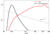 |
Fig. B.1 Radial profiles of normal optical depth in the Zodi run (red lines) and an additional Zodi run without rebounding collisions (black). An idealized profile (Eq. 15) is shown for comparison. |
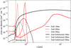 |
Fig. B.2 Size distribution of small grains (s < 10 µm) in the Zodi run (red lines) and an additional Zodi run without rebounding collisions (black) at three selected distances: 100 au (solid lines), 200 au (dashed), and 300 au (dotted). |
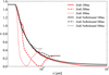 |
Fig. B.3 Average eccentricity in the Zodi run with rebounding collisions (red lines, same as in Fig. 7) and without them (black lines) plotted against particle size at different distances. |
Figure B.1 compares the optical depth profiles for the Zodi run with and without rebounding collisions. Without rebounding collisions, the optical depth profile exhibits the “normal” decrease with stellocentric distance. Figure B.2 shows the size distribution in the two runs. The most visible difference is that without rebounding collisions, the size distributions become smooth and similar to those in the Reference and Fomalhaut runs (cf. Fig. 7 left). In Fig. B.3, the mean eccentricities of different-sized particles with and without rebounding collisions are plotted, at several distances. The peculiar behavior described in Section 5.3 disappears when rebounding collisions are switched off. These results demonstrate that rebounding collisions, as opposed to disruptive ones, are the dominant collisional outcome in the Zodi run.
Appendix C Circular orbits in the outer disk
Here we investigate in more detail the collisions in the outer disk of the Reference and Zodi runs, in order to get more insights into the absence of circular orbits in the former one and their presence in the latter.
We first remind the reader how ACE simulations work. All disk particles are distributed into a three-dimensional grid of bins (m, q, e), where m is the mass of a particle, q the pericenter distance of its orbit, and e the orbital eccentricity. For every pair of bins, collisions with four collisional outcomes can occur: disruptive, cratering, rebounding, and sticking (eqs. 5–12), of which only the former three are relevant for our simulations. When a collision happens, the two colliders are removed from their bins and the appropriate bins are incremented to accommodate the particles created in that collision. Each of those collision types can happen a certain number of times during one time step, which associates each collision type with a certain collision rate.
As an example, we consider 0.9 µm particles with pericenters at 100 au and apocenters at 200 au, giving us an eccentricity of e = 1/3. (Note that, due to the discrete grid of the simulation, we actually consider the bin s = 0.93 µm, e = 0.35, q = 102 au.) This bin was chosen because in the Zodi run 0.9 µm-sized particles get in circular orbits of radius 200 au (see Fig. 7). We wish to see further evidence of the existence of these orbits in the Zodi run, as well as the absence thereof in the Reference one. Collisions experienced by the grains in that bin are visualized in Fig. C.1 as a heatmap2. It shows how often collisions in the bin occur with projectiles of different sizes and pericenter distances, and what the typical eccentricities of those impactors are.
We start by discussing the Reference run (Fig. C.1 left). Inspecting how the bins are incremented and decremented, we found that the (s = 0.93 µm, e = 0.35, q = 102 au) ring experiences all relevant collisional outcomes – destructive, cratering, and rebounding. This means that in the Reference run, collisions efficiently reduce particle mass, creating fragments that are too small to get injected by radiation pressure in circular orbits. Interestingly, the map demonstrates that the halo particles in the Reference run get destroyed by highly eccentric particles with various sizes and various pericenter distances – predominantly by ∼0.5 µm-sized particles with pericenters in the main belt and very high eccentricities.
We now consider the Zodi run. Our analysis of the bin evolution confirmed that only rebounding collisions are at work, as dust in the bin in question is too hard to undergo destructive and cratering collisions. Rebounding collisions gradually erode the grains, slightly reducing their sizes. In particular, they produce the particles with β = β′ (Eq. 18), which get in circular orbits. The heatmap in Fig. C.1 (right) also shows that the vast majority of collisions experienced by the halo particles in the (s = 0.93 µm, e = 0.35, q = 102 au) bin – i.e., those that act as a source for the circular orbits 200 au in radius – are particles that have different sizes, but all move in nearly circular orbits of different radii in the outer disk.
In addition to the already mentioned differences between the two heatmaps, it is clearly visible that there are many more collisions happening in the Zodi run than in the Reference one. This is because there are more small dust particles that act as possible collision partners in the Zodi run, in particular near the apocenter at 200 au where the collisional rates are highest.
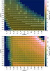 |
Fig. C.1 Collisions that remove particles from the (s = 0.93 µm, e = 0.35, q = 102 au) bin at T = 100 Myr in the Reference (left) and Zodi runs (right). The vertical and horizontal axes are the pericenter distance q and size s of the grains that collide with grains in that bin, respectively. Colors represent the collisional rates. These rates are summed over all collision partner’s eccentricities, and the numbers in the bins represent the eccentricity of the projectile with the highest collision rate. Bins where the collision with the projectile with the highest collision rate is disruptive or cratering are hatched while the ones where it is rebounding are not. |
In some debris disks with CO gas detections, the scattered light intensity peaks somewhat farther out from the star than the thermal emission does, which is attributed to outward drift of small µm-sized grains by gas drag forces (see Milli et al. 2026, and Olofsson et al., A&A, submitted).
To minimize visual distortion, heatmaps in this study employ the perceptually uniform colormap batlow (Crameri 2023).
All Tables
All Figures
|
Fig. 1 Chosen |
| In the text | |
|
Fig. 2 Schematic of the four possible collisional outcomes, Eqs. (5)–(12). The “projectile” particle (the less massive of the two colliders, marked with “p” and shown in red), and the “target” one (the more massive one, “t,” in blue) collide to produce one or two remnants (“rem” or “rem, p” and “rem, t,” each having the color of its progenitor particle) and a cloud of fragments that may originate from both colliders (“frag,” shown in black). |
| In the text | |
|
Fig. 3 Dust mass evolution for the three runs. Dashed lines depict the original (unscaled) and solid lines the scaled versions of the runs. Only one curve is shown for the Reference run as the scaled and unscaled versions are equivalent here. |
| In the text | |
|
Fig. 4 Time evolution of disk brightness in all three runs at 1 µm (dashed lines) and 1 mm (solid lines). |
| In the text | |
|
Fig. 5 Size distribution at 100 au in the three runs in the initial state (thin lines) and at T = 100 Myr (thick lines). |
| In the text | |
|
Fig. 6 Radial profiles of normal geometrical optical depth in the three runs. An idealized profile (Eq. (15)) and is shown for comparison. Both axes are logarithmic. |
| In the text | |
|
Fig. 7 Size distribution of dust grains (left) and average eccentricity of different-sized dust grains (right) in the Reference, Fomalhaut, and Zodi runs at three selected stellocentric distances: 100 au (solid lines), 150 au (dashed), and 200 au (dotted). Note that only dust grains smaller than 10 µm are shown. In both panels, the blowout grain size is marked with a vertical black line. |
| In the text | |
|
Fig. 8 Schematic of the proposed circularization mechanism. Black, the parent belt; blue, a halo grain; red, a secondary debris particle in a circular orbit. |
| In the text | |
|
Fig. 9 Peak positions of cross-section density distributions of the Zodi run as functions of distance from the star at three different system ages. Overplotted in black is the theoretical curve, Eq. (18). |
| In the text | |
|
Fig. 10 Thermal emission SEDs in the three runs analyzed (colored lines). The hatched regions indicate the portion of the SEDs generated by the part of the disk outside of 150 au. The black line is the stellar photosphere. |
| In the text | |
|
Fig. 11 Profiles of disk brightness (per pixel) in the three runs after 100 Myr of evolution, at wavelengths of 1 µm (dashed) and 1 mm (solid lines), using a resolution of 1 au/pixel. |
| In the text | |
|
Fig. B.1 Radial profiles of normal optical depth in the Zodi run (red lines) and an additional Zodi run without rebounding collisions (black). An idealized profile (Eq. 15) is shown for comparison. |
| In the text | |
|
Fig. B.2 Size distribution of small grains (s < 10 µm) in the Zodi run (red lines) and an additional Zodi run without rebounding collisions (black) at three selected distances: 100 au (solid lines), 200 au (dashed), and 300 au (dotted). |
| In the text | |
|
Fig. B.3 Average eccentricity in the Zodi run with rebounding collisions (red lines, same as in Fig. 7) and without them (black lines) plotted against particle size at different distances. |
| In the text | |
|
Fig. C.1 Collisions that remove particles from the (s = 0.93 µm, e = 0.35, q = 102 au) bin at T = 100 Myr in the Reference (left) and Zodi runs (right). The vertical and horizontal axes are the pericenter distance q and size s of the grains that collide with grains in that bin, respectively. Colors represent the collisional rates. These rates are summed over all collision partner’s eccentricities, and the numbers in the bins represent the eccentricity of the projectile with the highest collision rate. Bins where the collision with the projectile with the highest collision rate is disruptive or cratering are hatched while the ones where it is rebounding are not. |
| In the text | |
Current usage metrics show cumulative count of Article Views (full-text article views including HTML views, PDF and ePub downloads, according to the available data) and Abstracts Views on Vision4Press platform.
Data correspond to usage on the plateform after 2015. The current usage metrics is available 48-96 hours after online publication and is updated daily on week days.
Initial download of the metrics may take a while.