| Issue |
A&A
Volume 707, March 2026
|
|
|---|---|---|
| Article Number | A209 | |
| Number of page(s) | 16 | |
| Section | Planets, planetary systems, and small bodies | |
| DOI | https://doi.org/10.1051/0004-6361/202558607 | |
| Published online | 13 March 2026 | |
Characterising injection signatures in Jupiter’s ultraviolet aurora using Juno observations
1
Laboratory for Planetary and Atmospheric Physics, University of Liège,
Liège,
Belgium
2
Institute for Space Astrophysics and Planetology, National Institute for Astrophysics (INAF-IAPS),
Rome,
Italy
3
Southwest Research Institute,
San Antonio,
TX,
USA
4
Aix-Marseille Université, CNRS, CNES, Institut Origines, LAM,
Marseille,
France
5
University of Minnesota,
Minneapolis,
MN,
USA
6
The Johns Hopkins University Applied Physics Laboratory,
Laurel,
MD,
USA
7
Department of Earth & Planetary Sciences, University of Hong Kong,
Hong Kong,
China
8
Laboratory of Optical Astronomy and Solar-Terrestrial Environment, Institute of Space Sciences, School of Space Science and Technology, Shandong University,
Weihai,
Shandong,
China
★ Corresponding author: This email address is being protected from spambots. You need JavaScript enabled to view it.
Received:
17
December
2025
Accepted:
5
February
2026
Abstract
Discrete features in Jupiter’s ultraviolet aurora have been interpreted as signatures of plasma injections in the middle magnetosphere. There exists some ambiguity as to whether magnetodisc scattering or high-latitude Alfvénic acceleration best describes the observed properties of these injection signatures, and also the extent to which extent arcs in the outer emission are related to injections. Many injection signatures are the result of the evolution of dawn storms; however, there is limited evidence that non-dawn-storm injection signatures are sometimes present in the aurora. We use automatic detection of these discrete features, alongside data from Juno-UVS and in situ measurements by other Juno instruments, to show that scattering likely accounts for most of the electron precipitation associated with injection signatures. Additionally, there is evidence that injection signatures can be classified into two types: dawnstorm and non-dawn-storm. Arc-like features in the outer emission show very similar properties to traditional blob-like injection signatures and may consist of sequences of injection signatures that have broadened into an arc via energy-dependent electron drift.
Key words: planets and satellites: aurorae / planets and satellites: gaseous planets / planets and satellites: magnetic fields
© The Authors 2026
 Open Access article, published by EDP Sciences, under the terms of the Creative Commons Attribution License (https://creativecommons.org/licenses/by/4.0), which permits unrestricted use, distribution, and reproduction in any medium, provided the original work is properly cited.
This article is published in open access under the Subscribe to Open model. This email address is being protected from spambots. You need JavaScript enabled to view it. to support open access publication.
1 Introduction
In the equatorward region or outer emission of Jupiter’s ultraviolet (UV) aurora, discrete or patch-like features are frequently observed that can be linked to plasma injections in Jupiter’s magnetosphere (Dumont et al. 2014). These plasma injections were first detected by the Galileo probe (Mauk et al. 1997) and are expected to arise from interchange instability, whereby hot plasma from the distant magnetosphere moves inwards to compensate for the outward flow of new plasma from Io (Paranicas et al. 1991). Plasma injections frequently, but not always (Haggerty et al. 2019), give rise to injection signatures in Jupiter’s UV aurora. These signatures typically have an amorphous or blob-like morphology and can on occasion emit more power than the main emission (Palmaerts et al. 2023). The prevailing understanding suggests that anisotropic electron distributions induced by interchange events (injections) favour the production of plasma waves in the equatorial plane (Daly et al. 2023). These waves impose isotropic pitch-angle scattering on the magnetospheric electrons, filling the loss cone, leading to electron precipitation in the ionosphere, and hence auroral emission (Li et al. 2021), which has been directly observed in a young plasma injection by Juno (Menietti et al. 2021). However, an alternative high-latitude mechanism has been suggested to explain certain characteristics of injection signatures (Gray et al. 2017; Dumont 2023) and could provide sufficient energy flux to power the equatorward aurora (Gershman et al. 2019). In this second scenario, changes in the magnetic-field topology induced by an injection may launch Alfvén waves towards the ionosphere, where they accelerate electrons at high latitude and provoke auroral emission (Gray et al. 2017). It is not yet entirely clear to what extent these two mechanisms contribute to injection signatures; the diffuse aurora, in which injection signatures are sometimes embedded, appears to some extent to result from high-latitude Alfvénic acceleration, at least at low electron energies (Sulaiman et al. 2022; Kruegler et al. 2025). A third scenario, in which field-aligned electrical currents created by the accumulation of charge on the flanks of plasma injections give rise to injection signatures (Radioti et al. 2010), analogous to the terrestrial case (Chen & Wolf 1993), has also been suggested, though the absence of inverted-V potential structures in the middle equatorial magnetosphere (Salveter et al. 2022) makes this scenario unlikely. In the scattering scenario, the electron population is expected to become more isotropic under the effects of pitch-angle scattering (Li et al. 2017), and thus enhancements in the field-aligned electron flux should be accompanied by an enhancement in the perpendicular electron flux. Additionally, since the precipitating electron flux would be controlled by the loss-cone angle in the ionosphere, the corresponding injection signatures should emit less power in regions of the ionosphere where the magnetic field is stronger, since this reduces the loss-cone angle (Gérard et al. 2013). In the high-latitude Alfvénic scenario, the electron acceleration is instead expected to be largely field-aligned (Saur et al. 2018), and thus not accompanied by perpendicular acceleration. Alfvénic acceleration is also expected to be more efficient at higher magnetic-field strength (Hess et al. 2013), and thus, contrary to the scattering case, injection signatures should emit more power where the ionospheric magnetic field is stronger. These characteristics provide us with metrics to determine the extent to which these two acceleration mechanisms contribute to injection signatures. Gérard et al. (2013) observed that the north-south power ratio for injection signatures was neither directly nor inversely proportional to the surface field-strength ratio and were thus unable to differentiate between the two scenarios, though this was based on a single observation.
Discrete features between the main emission (e.g. Grodent 2015) and the statistical Io footpath (e.g. Bonfond et al. 2017; Palmaerts et al. 2023) are observed at all System-III longitudes, at radial distances between 7 and 40 Jupiter radii (RJ), and have lifetimes greater than 45 minutes, compatible with Galileo observations of plasma injections and first leading to their identification as injection signatures (Dumont et al. 2014). In addition, an increase in the brightness of injection signatures was observed when the main emission was expanded (Tao et al. 2018; Nichols et al. 2017), consistent with increased mass loading of the plasma torus, more iogenic plasma to be evacuated, and thus enhanced hot plasma injections to balance the magnetic-flux outflow (Bonfond et al. 2012). This link between internal processes and plasma injections is strengthened by the appearance of large injection signatures during periods of solar-wind quiescence (Kimura et al. 2016). Since 2016, Juno traversals of plasma injections have permitted a direct comparison with auroral morphology and the confirmation that discrete features in the outer emission are likely linked to plasma injections (Nichols et al. 2023). Injection signatures are frequently observed to be approximately conjugate between hemispheres (Gérard et al. 2013), consistent with the assumption that they are produced along closed field lines in the magnetosphere (Nichols et al. 2023). In addition to ‘blob-like’ injection signatures, arc-like discrete features with isotropic electron distributions (Radioti et al. 2009) have also been identified that were not directly identified as injection signatures, despite being observed to enhance in brightness several days after plasma injection (Gray et al. 2017).
Injection signatures are often associated with dawn storms in the UV aurora (Bonfond et al. 2021). Dawn storms are very bright discrete features coincident with the dawn-side main emission that arise from dipolarisation in the dawn-side magnetosphere, provoked by reconnection in the magnetotail, which itself gives rise to plasma injections in the post-noon sector (Yao et al. 2020; Bonfond et al. 2021). Ebert et al. (2021) associated auroral dawn storms with plasma injections and field-aligned currents. However, injections are only the final step of the dawn storm evolution track; an active dawn storm is more likely associated with dipolarisation rather than plasma injection (Bonfond et al. 2021), which may not energise auroral electrons via the same mechanisms. This transition from dawn storm has previously been reported from Hubble Space Telescope data (Gray et al. 2016). However, in one case, an injection signature was observed to arise in the absence of any preceding dawn storm (Bonfond et al. 2017). This hints that not all injections are the consequence of the evolution of dawn storms, though the limited number of observed cases makes it difficult to draw concrete conclusions. Indeed, quasi-constant small-scale-plasmoid or drizzle-like outflow have been suggested as mechanisms for outward mass transfer in the magnetosphere even in the absence of large-scale magnetotail reconfiguration (Bagenal 2007; Bagenal & Delamere 2011).
The outstanding questions in the literature that this work aims to tackle are thus: whether injection signatures can be classed into two types (dawn-storm and non-dawn-storm) based on their behaviour and characteristics; whether injection signatures are predominantly driven by scattering in the magnetodisc or high-latitude Alfvénic acceleration, and; whether there is a phenomenological difference between (blob-like) injection signatures and arcs in the outer emission. The Juno spacecraft, with its UV imager and suite of complementary instruments, is uniquely placed to improve our understanding of these aspects.
2 Observations
Composite UV images from the Juno UltraViolet Spectrograph (Juno-UVS) (68-210 nm; Gladstone et al. 2017) are used in this work. Juno’s highly elliptical polar orbit allows it to view Jupiter’s aurora in both hemispheres. Since Juno is a spin-stabilised spacecraft, Juno-UVS observes ‘strips’ of Jupiter’s aurora as the spacecraft rotates that can be collaged to create maps of the aurora. For each pass of the Juno spacecraft over Jupiter’s poles (a perijove; e.g. PJ1-N for perijove 1, northern hemisphere), an exemplar map was produced by collating a 100-spin (~50-minute) stack of Juno-UVS data that is centred as close as possible to the perijove time whilst covering at least 75% of the auroral region (Bonfond et al. 2018). Radiation noise from the impact of high-energy electrons on the detector is also removed (Bonfond et al. 2021). A more detailed description of the production of this exemplar map is given in Head et al. (2024). This results in a representative view of the aurora in each hemisphere during each perijove, though care must be taken when interpreting these exemplar maps. Different parts of the same feature may be sampled by spins that differ by 50 minutes, which may smear non-corotating auroral features. When the fine detail of features is being investigated, or comparisons drawn between auroral morphology and instantaneous in situ measurements, a ten-spin moving-window stack of Juno-UVS maps is more appropriate; this is mentioned where relevant in the text.
In addition to image data from Juno-UVS, data from the FluxGate Magnetometer (MAG-FGM; Connerney et al. 2017) and the Juno Energetic-particle Detector Instrument (JEDI; Mauk et al. 2017a) on board Juno are used. Technical details of each instrument are contained within their associated reference.
3 Methods
For this work, it is essential to have reliable estimates for the locations and shapes of injection signatures in UVS images of the aurora. To this end, an injection-detection pipeline was developed that uses manual designations of injection-signature locations to train a pixelwise random-forest classifier (Ho 1998). This benefits from the accuracy of the manual designations whilst incorporating the objectivity of the automatic classifier. A full description of this pipeline is given in Appendix A. These detected discrete features were further sub-divided into three categories based on their shape when projected from the ionosphere into the magnetosphere equatorial plane:
Small blobs: longitudinal extent <30°, radial extent <5 RJ;
Large blobs: longitudinal extent <30°, radial extent >5 RJ;
Arcs: longitudinal extent >30°, radial extent <5 RJ.
The radial-extent cutoff of 5 RJ was chosen to coincide with the ‘compact-structure’ latitudinal-width cutoff (3°; 1° latitude ~ 1.75 RJ in the outer emission) used in Dumont et al. (2014). The longitudinal-extent cutoff was selected qualitatively to differentiate between obvious arcs and more compact structures. A sensitivity analysis to support the use of this cutoff, in the context of the analysis surrounding Fig. 2, is given in Appendix B. A case showing the three types of feature morphology is given in Fig. 1.
Perijoves 1-40 are considered in this work. The evolution of Juno’s orbit is such that passes over the northern aurora occurred at increasing speed and passes over the southern aurora at increasing altitude towards later perijoves. This resulted in a diminishing UVS coverage of the aurora in the north and a diminishing resolution in the south, both of which hamper the reliable identification of injection signatures. As such, perijove 40 represents a reasonable cutoff for this work. In total, this corresponds to 78 exemplar maps of the aurora (Sect. 2), one per hemisphere per perijove excluding PJ2, when Juno was placed into safe mode. Exemplar maps of auroral brightness, B, in the non-absorbed (145-165 nm) band in Rayleigh were converted to maps of estimated emitted power, P, in watts by determining the surface area subtended by each pixel, A, and applying
 (1)
(1)
derived from the definition of the Rayleigh, where h is the Planck constant, c the speed of light, and 4.4 an empirical factor to convert the non-absorbed brightness into the full UV brightness (Groulard et al. 2024), calculated from a synthetic spectrum of H2 (Gustin et al. 2013; Hue et al. 2019). In this work, the nonabsorbed band was preferred over the more typical Lyman-α band (155-162 nm) because of its wider spectral range and hence greater signal-to-noise, especially to detect dimmer injection signatures. This estimation of emitted power in this wavelength band is very approximate and assumes that all UV photons have the same wavelength of |λ| = 160 nm. In this work, emitted power was only ever considered as the ratio of emitted power in the northern and southern hemispheres, and so the accuracy of the conversion is not essential as long as it is consistent between hemispheres.
In addition to maps of the auroral UV brightness, colour-ratio maps were also used in this work. The (methane) colour ratio is used to probe the average energy of precipitating electrons, which we take as the ratio of the intensity in the 155-162 nm and 135-140 nm bands, since this definition has been shown to be less sensitive to known calibration issues in Juno-UVS (Vinesse et al. 2026) than the typical (155-162)∕(125-130) nm definition (Gustin et al. 2013). In any case, Vinesse et al. (2026) indicate that the two colour ratios deviate mainly for very bright features (such as the main emission and dawn storms) and so the effect of this new colour ratio on our conclusions is expected to be slight, especially since the absolute value of the colour ratio is not used to draw conclusions in this work.
The auroral brightness at the Juno footprint was determined separately from the exemplar maps to ensure that the instantaneous brightness of the aurora below Juno is captured, since the exemplar maps represent a single snapshot of the aurora during Juno’s traversal of each hemisphere. For the peak brightnesses (embodied by the 90th-percentile brightness seen during Juno crossings of a discrete feature), an additional geometric correction of r2, where r is the radial distance from the centre of Jupiter in RJ, has been applied. This is to compensate for the effect that Juno’s altitude has on peak brightness; while the loss of resolution at higher altitudes should not affect the total power of an injection signature, the peak brightness value will decrease as r−2.
The downward (planetward), upward, and perpendicular electron energy flux was determined from JEDI data accessed via the JMIDL tool provided by John Hopkins University. Typically, JEDI data would be taken in conjunction with JADE data, which can sample lower-energy electrons than JEDI; however, since we used detected electron properties to calculate the total energy flux, JEDI higher-energy electrons contribute far more to the energy flux than the JADE lower-energy electrons, and so we consider this a reasonable simplification, used in previous work (e.g. Clark et al. 2018). Nevertheless, it should be stated that the electron energy fluxes presented in this work therefore represent lower limits, as per Clark et al. (2018). The downward and upward fluxes take electrons within 20° of the local magnetic-field vector, whereas the perpendicular flux takes electrons in the 45-135° range. This is to ensure that the loss cone is never sampled by the ‘perpendicular’ electron flux, since a loss-cone angle of 45° corresponds to an altitude of ~0.26 RJ, below the minimum Juno-crossing altitude for the injection signatures presented in this work. An approximate loss-cone angle of 20° is reasonable for Juno’s low-altitude passes over the aurora (Mauk et al. 2017b), though the exact angle varies with altitude and local surface magnetic field. Since it would be prohibitively time-consuming to download electron-flux data within the exact loss-cone angle for each timestamp during each perijove, a geometric correction is applied by multiplying the 20° electron energy flux by the ratio between the calculated loss-cone angle at each point during Juno’s traversal and 20°. This is a simple correction that does not take into account, for example, the potential inhomogeneity of the flux within the loss cone, but it is necessary to get reasonable estimates of the loss-cone electron flux from JMIDL data. In any case, perfect estimation of the losscone electron flux is difficult due to the lack of sampling by the most-field-aligned JEDI channels (Mauk et al. 2017b; Clark et al. 2018).
Alfvénic Poynting flux was determined from Juno-FGM data extrapolated via magnetic-flux conservation to the assumed auroral altitude of 400 km to ensure that the flux within the flux tube is correctly compared between perijoves regardless of Juno’s observing altitude, after the method presented by Gershman et al. (2019). A bandpass frequency filter with limits of (0.2, 5) Hz was applied to high-resolution (64 Hz; Connerney et al. 2017) Juno-FGM data; these filter frequencies were chosen to investigate Alfvén waves that could potentially give rise to auroral electron precipitation (Lorch et al. 2022). This filtered magnetic-field data was compared to the JRM33 magnetic-field model to determine the field residual, δB, and hence estimate the Alfvénic Poynting flux in this frequency range:
 (2)
(2)
where μ0 is the permeability of free space, as per Gershman et al. (2019).
Magnetic-field-line tracing was performed using the 18th-order JRM33 internal-field model (Connerney et al. 2022) combined with the Con2020 external-field model (Connerney et al. 2020), via routines made available by the JupiterMag Python library (James et al. 2022; Wilson et al. 2023). Field-aligned currents were calculated from FGM data compared against the above magnetic-field model and extrapolated via conservation of current to the assumed auroral altitude of 400 km as per Al Saati et al. (2022); a full description is given in Appendix A.2 of Head et al. (2025).
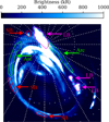 |
Fig. 1 Exemplar map of UV brightness from PJ7-N, saturated to highlight injection signatures. Automatically detected features in the outer emission have been highlighted according to their feature type as defined in the text: red = small blob (SB), magenta = large blob (LB), green = arc. Gridlines are in jovicentric coordinates and are spaced by 15° in latitude and longitude. |
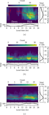 |
Fig. 2 Histogram in radial distance and local time of the projected extent in the equatorial plasma sheet of (a) large blobs, (b) small blobs, and (c) arcs in the outer emission. The mean-average location for each local-time bin is given by the red line; error bars denote the standard deviation. Histograms flattened in local time and radial distance are given to the bottom and right of the main plot, respectively. |
4 Results
4.1 Juno-UVS analysis
Via magnetic mapping into the equatorial plasma sheet, the magnetospheric location of injection signatures can be investigated, as is shown in Fig. 2; ‘Count’ denotes the number of different signatures that cover a given bin, though a single signature can cover multiple bins in the magnetosphere. Figure 2a indicates that large-blob features predominantly map to the dusk-side magnetosphere between 10 and 20 RJ from Jupiter. This radial distance is compatible with the preferred distance for young plasma injections identified by Juno (~17 RJ; Daly et al. 2024). The location of these large-blob features in the dusk-side magnetosphere is consistent with their interpretation as evolved dawn storms (Bonfond et al. 2021); as dawn storms evolve, they move duskwards and equatorwards, transforming into injection signatures in the dusk-side outer emission. This interpretation is strengthened by the fact that the average projected radial distance of the features decreases when moving from midday into dusk, as dawn storms leave the main emission and move equatorwards in the midday sector (Bonfond et al. 2021). The absence of these features in the dawn-side outer emission therefore strengthens the link between large injection signatures and evolved dawn storms, which remain coincident with the main emission in the dawn sector and only transform into large injection signatures once they leave the main emission in the post-noon sector (Bonfond et al. 2021).
As is shown in Fig. 2b, small-blob features are observed much more uniformly at all magnetic local times (MLTs), though there is still a slight preference for the dusk- and night-side aurora. Additionally, their projected radial distance is closer to Jupiter than that of big-blob features, forming a dense population around 11 RJ in agreement with earlier work (Dumont et al. 2014). It is curious that a significant portion of the small-blob population is located in the dawn side aurora, since dawn storms are expected to give rise to injections in the post-noon, dusk, and night sectors (Bonfond et al. 2021). This may be the result of a second class of injections that occur at all MLTs. Arc-like features in the outer emission show a very similar distribution as small-blob features (Fig. 2c), being concentrated around a radial distance of 11 RJ. Their distribution in MLT, while more uniform than the large-blob injection signatures, is decidedly biased towards the dusk-side aurora when compared with the small-blob features. The consequences of these results are discussed further in Sect. 5.
In addition to the example given by Bonfond et al. (2017), this work identifies several further cases of injection signatures that appear in the absence of a preceding dawn storm; an example from PJ6-S is given in Fig. 3. Here, at 06:51, the injection signature is barely present in the aurora, with a brightness comparable to the background brightness provided by the diffuse emission. Later, at 07:17, the power of the injection signature has increased threefold and now forms a clear, discrete structure distinct from the diffuse emission. This example is present in the post-noon aurora (−13 MLT); two further examples in Figs. E.1 and E.2 are located at ~9 MLT and ~11 MLT, respectively, indicating that non-dawn-storm injections may occur at a variety of local times.
Figure 4 shows the shift between the brightness peak and colour-ratio peak for blob-like injection signatures. A positive (negative) shift indicates that the brightness peak is at higher (lower) System-III longitude than the colour-ratio peak. These shifts were calculated from the ten highest-resolution (lowest-altitude) consecutive Juno-UVS spins that captured at least 90% of the injection signature; signatures with fewer than ten consecutive spins were ignored. This is to avoid spurious shift measurements in cases in which the injection signature has not been sufficiently sampled by Juno-UVS either spatially or temporally. This method is preferred over the use of the exemplar maps to avoid introducing artefact brightness or colour-ratio peaks, since the exemplar maps are built from spins that may sometimes differ considerably in time. Around half of detected injection signatures show no discernible shift between the brightness and colour-ratio peaks (absolute shift < 0.5°). These features are relatively uniformly distributed in MLT, and a homogeneity test (a two-sided t-test) between the feature counts in the dawn sector (3 MLT to 12 MLT; this choice is motivated by the empty region in Fig. 2a where large-blob signatures are absent) and the dusk and night (non-dawn) sectors (12 MLT to 3 MLT) returns a p value of 0.16. This is insufficient to indicate non-homogeneity at the 95% confidence level. Cases with noticeable shift have been separated into slight shifts (0.5° ≤ shift < 1°) and considerable shifts (shift ≥ 1°) to increase the granularity of the analysis. The negative-shift cases, which collectively account for 32% of all detected features, appear to be concentrated in the dusk sector between 12 and 21 MLT; the same homogeneity test indicates a probability of 95% that the negative-shift cases are not homogenous between the dawn and non-dawn sectors, which is a stronger indication of non-homogeneity than for the no-shift cases. Positive-shift cases only account for 15% of the detected injection signatures. Of the 20 cases with strong positive shifts (>1°), 18 were found to be due to misdetection by the peak-finding algorithm, typically because the closest colourratio peak to the brightness peak was significantly smaller than a more distant peak (or vice versa), or because a single brightness peak presents as two slightly separated colour-ratio peaks (or vice versa). This leaves only two signatures with strong (>1°) positive shifts that are not obviously the consequence of algorithmic failure. In both of these cases, however, the widths of the brightness and colour-ratio peaks show significant overlap. A similar inspection of the strong-negative-shift cases provides many more examples (36 out of 51 signatures, or 70%) of convincing negative shift; some examples are given in Figs. E.3 and E.4. This is as expected, since negative-shift cases correspond to injections where energy-dependent drift has forced the high-energy electrons (that give rise to the colour-ratio peak) ahead in System-III longitude of the lower-energy electrons (that, through a greater population, give rise to the brightness peak). Positive-shift cases are therefore difficult to describe in this framework, since our current understanding supposes that energy-dependent drift always pushes the high-energy electrons ahead of the low-energy electrons (Mauk et al. 2002) due to the properties of the energy-dependent drift imposed by curvature and gradients in the magnetic field (Mauk et al. 1999; Dumont et al. 2018). If we assume that all positive-shift cases are due to a deficiency in the algorithm, and that this deficiency works to introduce positive and negative artefacts symmetrically, we can subtract the positive-shift counts from the negative-shift counts to estimate the ‘true’ distribution. This returns a population of 75% no-shift features, 9% slight-negative-shift features, and 15% negative-shift features. Thus, even after we compensate for the deficiencies of the peak-detection algorithm, negative-shift cases still make up a significant portion (24%) of all injection signatures. Note that exact proportions of each shift type are dependent on the implementation of the peak-detection algorithm; nevertheless, it can be said that negative-shift cases likely constitute a non-negligible portion of all injection signatures.
One of the key observable differences between the magnetodisc-scattering and high-latitude-acceleration scenarios to precipitate electrons into injection signatures is the relation between injection-signature power and the local magnetic-field strength present for the injection signature within the ionosphere. In the latter case, a greater precipitating electron flux is expected in regions of higher surface field strength, due to increased efficiency of the Alfvénic acceleration process (Hess et al. 2013). However, in the isotropic-scattering case, the precipitating electron flux is controlled by the loss-cone angle in the ionosphere, and hence
 (3)
(3)
following the derivation given in Appendix C, where P is the emitted UV power, extrapolated from the power in the nonabsorbed band as per Sect. 3, and B the surface magnetic-field strength in the northern (N) and southern (S) hemispheres. Here, the ratio of auroral power between hemispheres is preferred to a direct comparison of auroral power with surface field strength to remove the influence of the intrinsic intensity of the plasma injection, the same for the injection signature in the northern and southern aurora, since this may otherwise mask the influence of surface field strength on injection-signature power. This analysis also supposes that conjugate injection signatures are sufficiently long-lived to remain visible in the southern hemisphere even after the approximately three-hour traversal of Juno between hemispheres, which is supported by previous work (Gérard et al. 2013; Dumont et al. 2018).
This theoretical relation is plotted in Fig. 5 alongside the observed hemispheric (north over south) power ratios for the injection signatures analysed in this work. Here, the pixel masks covered by the detected injection signatures (see Appendix A) in one hemisphere are projected along magnetic field lines to the other hemisphere, which creates a similar pixel mask in the other hemisphere. The total projected power can be calculated from this projected mask and compared to the total power in the original mask, though this assumes that the injection is in full corotation and produces conjugate signatures in both hemispheres. This means that most injections have two points in Fig. 5 (N→S, S→N), but both points are included to account for cases where the injection signature is detected in only one hemisphere. The projection of a detected injection signature into the other hemisphere is also preferred over a comparison of two conjugate detected signatures because the areas returned by the signature-detection algorithm may not be exactly conjugate between the two hemispheres, and some signatures may be missed entirely in one hemisphere. It is nevertheless expected that injection signatures be magnetically conjugate (Gérard et al. 2013), as seen frequently by Juno (e.g. Bonfond et al. 2017; Palmaerts et al. 2023). Of the injection signatures detected in this work, 33% were found to have at least 50% of their conjugate area covered by another detected injection signature. It is expected that this relatively low conjugate-detection fraction is a consequence of algorithmic failure and the longitude precession of the injections, rather than a genuine lack of hemispheric conjugacy.
It can be seen that the linear relation fitted to these points is very close to the theoretical scattering relation. However, there exists significant scatter in the data points, as evidenced by the low R2 value of 0.11. Firstly, a t-test was performed with the null hypothesis that the power ratios of points with (negative log2) field-strength ratios above zero are higher than those below zero. This led to a rejection of the null hypothesis with a probability of 10−13, indicating that the clustered population of points on the left of Fig. 5 are strongly suggested to have greater power ratios than those points on the right. This is not incompatible with the large scatter in Fig. 5; though the data in the left and right clusters show reasonable overlap in their (presumed Gaussian) power-ratio distributions, these distributions are sufficiently well sampled by the data to say with considerable certainty that data on the right are taken from a population with a lower average power ratio than the data on the left. Secondly, injections are known to slightly sub-corotate (Gérard et al. 2013; Dumont et al. 2018), and so will have moved slightly between Juno’s northern and southern pass. This may explain why the power contained within the other-hemisphere-projected injection-signature mask is consistently lower than the power within the original mask, regardless of in which hemisphere the original injection signature is detected; an injection signature may move enough between Juno’s northern and southern pass that a part of it lies outside the projected mask, reducing the total power within the mask. Taking a representative corotation of 85% (Dumont et al. 2018), an injection signature will have moved by ~14° between Juno’s northern and southern pass, which may be sufficient to explain the ~50% scatter (~1 on the y axis of Fig. 5) for injection signatures typically of comparable longitudinal extent. This possibility is investigated more rigorously in Appendix D, where it is shown that, for a typical injection signature, a slight subcorotation of 80-90% may largely explain the distribution of points in Fig. 5. These analyses increase confidence that the fitted relation in Fig. 5 reflects physical reality, though the extent to which this scatter can be accounted for by the results of these analyses is difficult to estimate. It should be noted that, while these caveats exist for the interpretation of the fitted relation in Fig. 5, positive correlation between increased field-strength ratio and power ratio, and hence high-latitude Alfvénic acceleration within injection signatures, is not supported by Fig. 5.
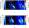 |
Fig. 3 Injection signature observed on May 19, 2017, at (a) 06:51:03 and (b) 07:17:19 by Juno-UVS during PJ6-S, highlighted in green. The brightness map is given on the left and the colour-ratio map on the right. The main emission is present to the right of the injection signature. |
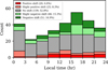 |
Fig. 4 Histogram in magnetospheric local time of (small and large) blob-like injection features in the outer emission. Features are categorised by the magnetospheric longitude shift between the brightness peak and colour-ratio peak: no shift (<0.5°), slight shift (0.5° to 1°), and shift (>1°), from positive (red, bottom) through to negative (green, top) shifts. |
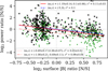 |
Fig. 5 North-to-south UV auroral power ratio vs surface magnetic-field-magnitude ratio for injection signatures detected by Juno-UVS during the first 40 perijoves. The N→S projections are denoted by black ×, and the S→N projections by green +. The best-fit linear relation for all points is given by a solid red line, and separate fitted relations for the N→S and S→N case by dotted and dash-dotted lines, respectively. The theoretical pitch-angle-scattering relation is given by a dashed blue line. |
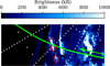 |
Fig. 6 Juno footprint path (green) overlaid on the exemplar map of the aurora for PJ21-N. An automatically detected small-blob-type discrete feature crossed by Juno is highlighted in red. The direction of travel of Juno is denoted by the green arrow. |
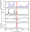 |
Fig. 7 Juno instrument data for PJ21-N. The crossing of the discrete feature in Fig. 6 is given in red. From top to bottom: JEDI field-aligned (0°-20° upwards, 160°-180° downwards) electron energy flux; UVS footprint brightness; calculated ionospheric field-aligned electrical current; calculated ionospheric Alfvénic Poynting flux. |
4.2 Juno multi-instrument analysis
In addition to the analysis of auroral maps made by Juno-UVS, the properties of injection signatures can be investigated using other instruments on board Juno. Figures 6 and 7 show the evolution of several calculated parameters as the Juno footprint passed through a blob-like injection signature during PJ21-N. The footprint UVS brightness was observed to peak within the range attributed to the feature crossing, which increases confidence that this feature is being properly detected. The field-aligned downward electron energy flux shows a small peak (~15 mW m−2) during the feature crossing, which is slightly below the energy flux expected to produce an auroral brightness of ~200 kR (20 mW m−2; Gérard et al. 2016). The dissipative Alfvénic flux also shows a clear peak far above the background level. A similar case where Juno instead flew over an arc-like feature (Figs. E.5 and E.6) shows very similar behaviour.
When considering Juno crossings of both blob-like and arclike discrete features in the outer emission during the first 40 perijoves, there exists a noticeable correlation between the downward electron-energy flux measured by JEDI and the instantaneous Juno-footprint auroral brightness, as given by the solid black line in Fig. 8. However, while high electron-energy flux (≳80 mW m−2) can be robustly associated with high auroral brightness (≳800 kR), the R2 value of only 0.32 does not strongly support the fitted linear relation, and there exist several injectionsignature crossings where high auroral brightness was coincident with only modest downward electron flux. Several mitigating factors exist that may partially explain this discrepancy. Firstly, the most field-aligned electrons are often poorly sampled by the JEDI instrument (Mauk et al. 2017b). This can lead to an underestimation of the field-aligned electron energy flux, and one that is inconsistent between injection-signature crossings. Secondly, while, for a typical average electron energy of 100 keV, the expected relation between electron energy flux and auroral brightness is 1 mW m−2 - 10 kR, this relation can vary slightly with electron energy (Gustin et al. 2016), which may work to disrupt any linear relation that would otherwise be expected in Fig. 8. Finally, the loss-cone correction applied to the electron flux (described in Sect. 3), while necessary to extrapolate the electron flux within 20° to the loss-cone electron flux at Juno, may also introduce some artificial error, especially when this relatively coarse correction is applied where the loss-cone angle differs significantly from 20°, though it should be noted that this correction improves the strength of the linear relation in Fig. 8 (R2 = 0.11 → 0.32). With these caveats in mind, the principle that an increased downward electron energy flux leads to a higher auroral brightness is somewhat supported by Fig. 8. Figure 8 also shows no meaningful separation between blob-like and arclike discrete features in the outer emission. Both morphologies occupy the same regions of the plot, and the fitted linear relations are identical within the calculated uncertainties. This indicates that blob-like and arc-like outer-emission features have similar typical ratios between brightness and electron flux, and hence a similar range of typical electron energies.
As is shown in Figs. 9 and 10, there exist also moderately strong linear relations between the upward and downward, and downward and perpendicular, electron energy fluxes. Here, ‘upward’ and ‘downward’ refer to the electron population within 20° of the local magnetic-field vector, without the loss-cone correction as described in Sect. 3. ‘Perpendicular’ electrons have pitch angles between 45° and 135°. The lack of loss-cone-angle correction is to be able to compare the (fixed-angular-width) perpendicular electron flux with other parts of the pitch-angle profile, rather than to compare the auroral brightness with the precipitating electrons that give rise to it, as in Fig. 8. In any case, the effect of this correction on Figs. 9 and 10 is minimal. The reasonable correlation between all three portions of the directional electron flux indicates that the electron acceleration is likely to be, for the most part, isotropic and not simply bidirectional and field-aligned. This is more compatible with magnetodisc scattering to provoke auroral electron precipitation (Li et al. 2017), rather than high-latitude field-aligned acceleration, discussed further in Sect. 5.
The full average electron pitch-angle profiles (in log10 to highlight order-of-magnitude differences and normalised to prevent dominance of the greatest absolute electron flux in the average profile) for both blob-like and arc-like features (Fig. 11) show butterfly distributions (Ma et al. 2017), which indicate the same loss-cone depletion as pancake distributions (Salveter et al. 2022) but also include a ‘notch’ at 90°. This notch is tentatively associated with a slight parallelisation of a pancake distribution via Landau damping of electrostatic waves at low altitude (Ma et al. 2017). Alternatively, Sulaiman et al. (2022) suggest that this notch be likely unphysical and related to spacecraft shadowing effects (Sulaiman et al. 2022). From Fig. 11, it would appear that there is no significant difference in the average electron pitch-angle profiles of blob-like and arc-like features in the outer emission. Additionally, the pancake-like butterfly distribution shown by both types of feature is indicative of partial refilling of the loss cones by isotropic scattering (Salveter et al. 2025), which implies that the two corresponding source processes are at least comparable, if not the same process.
Similarly, the Alfvénic Poynting flux (in the potentially dissipative frequency range of 0.2-5 Hz; Lorch et al. 2022) observed during Juno crossings of injection signatures shows a reasonable linear correlation with auroral brightness, as in Fig. 12. It should be noted that Fig. 12 only includes cases where the Juno crossing occurred below an altitude of 1 RJ, since no peaks in the Alfvénic flux were observed above this altitude. Additionally, to ensure a sensible comparison between data points, cases where the Juno crossing occurred in a region of magnetic field strength above 0.1 mT (where Juno-FGM has a higher operational range than during the rest of a pass over the aurora; Connerney et al. 2017) have been ignored. Here, unlike in Fig. 8, there appears to be a separation between arc-like and blob-like features, with the high-flux, high-brightness populated predominantly by blob-like features. Given the lack of such a separation in Fig. 8, it is anticipated that this is a result of the stricter filters for feature crossings in Fig. 12 and low-number statistics rather than a physical effect. In any case, there remains a reasonable (R2 = 0.52) correlation between Alfvénic Poynting flux below 1 RJ and feature brightness for ‘traditional’ blob-like injection signatures. Since this Alfvénic flux is still observable at low altitudes, and therefore not consumed by wave-particle interactions as expected for the main emission (Sulaiman et al. 2022), we suggest that it does not contribute significantly to the electron precipitation associated with injection signatures and may instead be a by-product of the pitch-angle scattering process.
Similar to the Alfvénic flux, the magnitude of the upward electrical currents (that correspond to a majority of downward travelling electrons) also show some measure (R2 = 0.32) of correlation with observed auroral brightness for the discrete outer-emission features investigated in this work. This is as expected for plasma injections; a parcel of plasma moving within a magnetic field will naturally lead to the production of electrical currents (Radioti et al. 2010). We may also expect that whichever property (or properties) of the plasma injection governs the brightness of the corresponding injection signature may also govern the intensity of the produced electrical currents. However, similarly to the Alfvénic flux discussed above, correlation between upward current density and auroral brightness does not necessarily imply a current-based origin for injection signatures, as discussed further in Sect. 5.
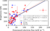 |
Fig. 8 90th-percentile brightness vs 90th-percentile precipitating energy flux based on downward JEDI electrons (25-1000 keV) observed by Juno during crossings of arc-like (blue) and blob-like (red) features in the outer emission. Error bars denote the 80th-100th percentile range. The best-fit linear relation is given by a solid black line, as well as separate best-fit relations for the arc-like (dashed) and blob-like (dash-dotted) features. The theoretical relation after Gérard et al. (2016) is given by the dotted grey line. |
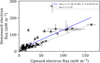 |
Fig. 9 90th-percentile upward vs downward electron energy flux observed by JEDI during crossings of discrete features in the outer emission. Error bars denote the 80th-100th percentile range. The bestfit linear relation is given by a solid blue line, and the 1:1 relation by a dashed grey line. |
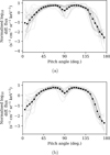 |
Fig. 11 Average electron pitch-angle distribution observed by JEDI during crossings of (a) blob-like and (b) arc-like features in the outer emission. Pitch-angle distributions from individual crossings are given in light grey. 0° (180°) denotes downward (upward) field-aligned electron flux. |
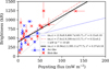 |
Fig. 12 90th-percentile brightness vs 90th-percentile ionospheric Alfvénic flux extrapolated from Juno(-UVS, -FGM) observations below an altitude of 1 RJ during crossings of arc-like (blue) and blob-like (red) features in the outer emission. Error bars and best-fit relations are denoted as per Fig. 8. |
5 Discussion
This work presents evidence that there may exist two classes of auroral injection signature, and hence two classes of injection. The first, that we refer to as dawn-storm injections, is that of dawn storms that evolve through the large-blob phase and become smaller injection signatures. We would expect these injection signatures to be found in the post-noon, dusk, and night sectors (Bonfond et al. 2021) as the (sub-)corotating dawn storms move duskwards as they evolve. We would also expect these dusk-side injection signatures to show signs of ageing via energy-dependent electron drift (Bonfond et al. 2017). The second is injection signatures that arise even in the absence of dawn storms. The onset of a non-dawn-storm injection signature has been observed in only a single case prior to this work (Bonfond et al. 2017), perhaps owing to their relatively short onset time compared to the typical lifetime of an injection signature. This work (Figs. 3, E.1, and E.2) provides further examples of this phenomenon, indicating that the case presented by Bonfond et al. (2017) was not a one-off event. Indeed, the example given in Fig. 3 is a small feature with no discernable shift between the brightness and colour-ratio peaks, indicative of a ‘young’ injection. We suggest that these smaller non-dawn-storm injection signatures arise at all MLTs and therefore account for the considerable population of injection signatures in the dawn-side aurora; the dusk-side aurora thus consists of a mixture of the two types of injection signature. This interpretation is consistent with the local-time distribution of injection signatures (Fig. 2). Large-blob injection signatures are found exclusively at dusk because dawn storms evolve into injection signatures in this sector (Bonfond et al. 2021), and small-blob injection signatures show a uniform distribution of non-dawn-storm injection signatures overlain by dusk-side dawn-storm injection signatures. This is compatible with the distribution of brightness and colour-ratio shifts (Fig. 4), which shows a uniform no-shift baseline for the young non-dawn-storm injections and a dusk-side concentration of negative-shift cases for the aged dawn-storm injection signatures. The existence of non-dawn-storm injections at any local time may be consistent with a finger-like, interchange-dominated magnetodisc structure (Feng et al. 2023; Yao et al. 2025) and/or the presence of reconnection events identified at all local times in the magnetodisc (Guo & Yao 2024; Zhao et al. 2024). Alternatively, the dawn-side population of no-shift injection signatures may be explained by the existence of significantly aged dawnstorm injections that have remained detectable and sub-corotated into the dawn-side aurora; in this scenario, the high-energy electron population may be completely depleted, which would bring the colour-ratio peak back in line with the brightness peak. However, the threefold increase in auroral power over a timescale of hours for the dawn-side examples given in Figs. 3, E.1, and E.2 is not easily compatible with significantly aged injection signatures arising from later-stage injections, since we would not expect these to increase in brightness at such a late stage in their evolution. More work is required regarding the distribution, properties, and evolution of injections to be able to differentiate between these two scenarios.
The results of this work do not support high-latitude Alfvénic acceleration as the dominant mechanism for the production of injection signatures. Firstly, the butterfly pitch-angle distributions (Fig. 11) and the correlation between the downward, upward, and perpendicular flux in the low-altitude electron populations above injection signatures (Figs. 9 and 10) are consistent with an isotropic acceleration process, such as pitch-angle scattering in the magnetodisc, rather than a largely field-aligned process, as high-latitude Alfvénic acceleration (and, indeed, acceleration via electrical currents; Ebert et al. 2021) is expected to be. This interpretation is strengthened by the lack of a positive correlation between hemispheric surface-field and auroral-power ratios for injection signatures, as would be expected for high-latitude Alfvénic acceleration. Indeed, Fig. 5 shows some evidence for the inverse-log proportionality expected of isotropic scattering, though the dispersion in the data prevents us from drawing concrete conclusions from this analysis alone. Finally, the existence of injection signatures with upstream drift of their colour-ratio peak (Fig. 4) is far more consistent with the isotropic scattering of an energy-differentiated (aged) plasma injection than with high-latitude Alfvénic acceleration (Dumont et al. 2018). Dumont (2023) suggests that more no-shift (young) injection signatures are detectable at higher surface field strength in the north, whereas this distribution is more uniform in the south, which was suggested to be the consequence of Alfvénic acceleration and its positive correlation between surface magnetic-field strength and auroral brightness. We suggest instead that no-shift injection signatures are biased at high surface field strength (the maximum surface field strength is higher in the north) because a stronger surface field reduces the size of features in the ionosphere and thus makes it more difficult to identify non-zero brightness and colour-ratio peak shifts with the finite spatial resolution of Juno-UVS. It has also been suggested that modification of the local magnetic-field topology by a plasma injection may produce Alfvén waves (Gray et al. 2017), which may be the source of the Alfvénic-flux peaks seen by Juno during traversals of injection signatures. However, since the evidence presented in this work indicates that pitch-angle scattering is the dominant acceleration process, it is unlikely that this Alfvénic flux, which is expected to produce field-aligned acceleration, contributes significantly to electron acceleration above injection signatures. Indeed, the fact that Alfvénic flux in the potentially dissipative regime (Lorch et al. 2022) is observable at low altitude above injection signatures at all indicates that this flux does not significantly contribute to electron acceleration. For example, the main emission, which is more frequently attributed to Alfvénic acceleration in recent years (e.g. Sulaiman et al. 2022; Head et al. 2024; Kruegler et al. 2025), is not associated with significant Alfvénic flux at low altitude (Sulaiman et al. 2022); instead, dissipative Alfvénic flux is observable at ~ 10 RJ (Lorch et al. 2022) that is then efficiently converted into electron acceleration at low altitude, resulting in bidirectional field-aligned electron distributions but no low-altitude Alfvénic flux. A similar scenario does not appear to be valid for injection signatures. The moderate correlation between Alfvénic flux and auroral brightness (Fig. 12) is perhaps indicative that the source process that isotropically scatters electrons in the equatorial plane also produces Alfvénic perturbations, the strength of which scales with the strength of the scattering process. Overall, the results of this work support pitch-angle scattering as the dominant mechanism for electron precipitation by plasma injections, consistent with previous work (e.g. Li et al. 2017; Dumont et al. 2018; Devinat et al. 2025).
Similarly, the correlation between upward electrical current density and auroral brightness shown in Fig. 13 reminds us that correlation between two parameters does not imply causality. Electrical currents, despite this correlation, are unlikely to be significant contributors to the electron precipitation associated with injection signatures; as discussed above, the ubiquity of electron pitch-angle distributions associated with isotropic scattering, as well the absence of inverted-V structures (Salveter et al. 2022), above injection signatures is inconsistent with precipitation from currents induced by quasi-static electrical potentials. We propose instead that plasma injections that give rise to injection signatures also produce field-aligned electrical currents due to charge accumulation on their flanks, as has previously been suggested (Radioti et al. 2010), but that these currents do not result in significant auroral precipitation.
This work also presents evidence that blob-like and arc-like discrete features in the outer emission are both governed by the same fundamental processes. Both feature types present comparable relations between downward electron flux or Alfvénic flux and auroral brightness (Figs. 8 and 12) and show near-identical average electron pitch-angle distributions (Fig. 11). Additionally, small blob-like and arc-like features are both projected to a preferred radial distance of ~11 RJ in the equatorial magnetosphere (Fig. 2). This indicates that there is some measure of similarity between blob-like and arc-like features in the outer emission. One key difference is that arc-like features seem to be less common in the dawn-side aurora. We suggest that these results may be explained if arc-like features are interpreted as sequences of broadened or ‘smeared-out’ blob-like features under the influence of energy-dependent electron drift, as is expected to occur (Dumont et al. 2018). Dawn storms are known to sometimes produce sequences of injection signatures in the post-noon sector (Bonfond et al. 2021). If these injections are sufficiently closely packed, energy-dependent electron drift may make it difficult to ascertain where one injection signature ends and the next begins. Importantly, only dawn-storm injection signatures would be expected to show sufficient dispersion during the aged small-blob phase to broaden into an arc, since we anticipate that non-dawn-storm small-blob injection signatures would decay below the detection threshold before sufficient broadening had occurred; in any case, it is not presently clear why these nondawn-storm injection signatures should occur in a sequence. This interpretation explains why arc-like and small blob-like injection signatures preferentially occur at the same radial distance, but why arc-like signatures are less forthcoming in the dawnside aurora, where dawn-storm injection signatures are absent. The extended ‘second auroral oval’ in the dawn-side aurora reported by Gray et al. (2017) observed five days after a series of exceptionally bright injection signatures may be explained if the exceptional brightness of these sequential injection signatures allows them to remain detectable even once they have sub-corotated into the dawn aurora, at which point they would be expected to have undergone significant energy-dependent drift and hence have formed an extended arc. The requirement for injection signatures to be initially exceptionally bright if they are to remain detectable once they reach the dawn-side aurora may explain the reduced (though still present) population of dawn-side arc-like features in Fig. 2c.
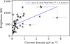 |
Fig. 13 90th-percentile brightness vs 90th-percentile upward ionospheric current density extrapolated from Juno(-UVS, -FGM) observations during crossings of discrete features below an altitude of 1 RJ in the outer emission. Error bars denote the 80th-100th percentile range. The best-fit linear relation is given by a solid blue line. |
6 Conclusions
In response to the three questions tackled by this work, presented in the introduction, we present the following results:
There is some evidence to suggest that injection signatures (and consequently injections) can be classified into two types: dawn-storm and non-dawn-storm. Dawn-storm injections occur primarily in the dusk and night sector and present as large, bright injection signatures that decay into smaller injection signatures that show ageing via energy-dependent electron drift. Non-dawn-storm injections can occur at any local time and present as small, unaged injection signatures. Dawn-storm injections occur over a range of radial distances (10-20 RJ), whereas non-dawn-storm injections appear to occur predominantly below 15 RJ, with a peak at 11 RJ;
Injection signatures appear to be dominated by pitch-angle scattering of electrons in the magnetospheric equatorial plane rather than by field-aligned currents or Alfvénic acceleration at high latitude. The low-altitude auroral electron energy flux increases isotropically with injection-signature brightness, and higher surface magnetic-field strength typically leads to a dimmer injection signature, consistent with pitch-angle scattering;
Arc-like discrete features in the outer emission may consist of sequences of dawn-storm injection signatures that have undergone broadening via energy-dependent electron drift. Juno crossings of both types of feature revealed no significant difference in their typical electron populations or Alfvénic flux. They map to the same radial distance as small blob-like features but are more preferentially located in the dusk-side aurora, consistent with injection signatures resulting from dawn storms.
Further work should aim to identify further examples of nondawn-storm injection signatures and test whether they are truly uniformly distributed in local time, an analysis that is not possible at present due to the low number of conclusively identified non-dawn-storm injection signatures. Confirmed Juno crossings of non-dawn-storm injection signatures would also allow us to investigate whether the two classes of injection signature differ in their particle or wave or current properties, which would likely require a combination of in situ measurement and remote observation. A more extensive comparison of blob-like and arc-like discrete features, perhaps looking at the average energy of the precipitating electrons or an extended sequence of observations, may provide further evidence that arc-like features in the outer emission consist of sequences of broadened injection signatures.
Data availability
Juno data can be obtained from the NASA Planetary Data System (https://pds-atmospheres.nmsu.edu/data_and_services/atmospheres_data/JUNO/juno.html).
Acknowledgements
We are grateful to NASA and contributing institutions that have made the Juno mission possible. This work was funded by NASA’s New Frontiers Program for Juno via contract with the Southwest Research Institute. This publication benefits from the support of the French Community of Belgium in the context of the FRIA Doctoral Grant awarded to L.A. Head. B. Bonfond is a Research Associate of the Fonds de la Recherche Scientifique - FNRS. Data analysis was performed with the AMDA science analysis system provided by the Centre de Données de la Physique des Plasmas (CDPP) supported by CNRS, CNES, Observatoire de Paris and Université Paul Sabatier, Toulouse. A. Moirano is supported by the Fonds de la Recherche Scientifique - FNRS under Grant(s) No. T003524F. V. Hue acknowledges support from the French government under the France 2030 investment plan, as part of the Initiative d’Excellence d’Aix-Marseille Université - A*MIDEX AMX-22-CPJ-04, and CNES.
References
- Al Saati, S., Clément, N., Louis, C., et al. 2022, JGR: Space Phys., 127, e2022JA030586 [Google Scholar]
- Bagenal, F. 2007, J. Atmos. Sol. Terrestr. Phys., 69, 387 [Google Scholar]
- Bagenal, F., & Delamere, P. A. 2011, JGR: Space Phys., 116 [Google Scholar]
- Bonfond, B., Grodent, D., Gérard, J.-C., et al. 2012, GRL, 39 [Google Scholar]
- Bonfond, B., Saur, J., Grodent, D., et al. 2017, JGR: Space Phys., 122, 7985 [Google Scholar]
- Bonfond, B., Gladstone, G. R., Grodent, D., et al. 2018, GRL, 45, 12108 [Google Scholar]
- Bonfond, B., Yao, Z. H., Gladstone, G. R., et al. 2021, AGU Adv., 2, e2020AV000275 [CrossRef] [Google Scholar]
- Chen, C. X., & Wolf, R. A. 1993, JGR: Space Phys., 98, 21409 [Google Scholar]
- Clark, G., Tao, C., Mauk, B. H., et al. 2018, JGR: Space Phys., 123, 7554 [Google Scholar]
- Connerney, J. E. P., Benn, M., Bjarno, J. B., et al. 2017, Space Sci. Rev., 213, 39 [Google Scholar]
- Connerney, J. E. P., Timmins, S., Herceg, M., & Joergensen, J. L. 2020, JGR: Space Phys., 125, e2020JA028138 [Google Scholar]
- Connerney, J. E. P., Timmins, S., Oliversen, R. J., et al. 2022, JGR: Planets, 127, e2021JE007055 [Google Scholar]
- Daly, A., Li, W., Ma, Q., et al. 2023, GRL, 50, e2023GL103894 [Google Scholar]
- Daly, A., Li, W., Ma, Q., et al. 2024, GRL, 51, e2024GL110300 [Google Scholar]
- Devinat, M., André, N., Vinci, G., et al. 2025, GRL, 52, e2025GL116114 [Google Scholar]
- Dumont, M. 2023, PhD thesis, Université de Liège [Google Scholar]
- Dumont, M., Grodent, D., Radioti, A., Bonfond, B., & Gérard, J.-C. 2014, JGR: Space Phys., 119, 10068 [Google Scholar]
- Dumont, M., Grodent, D., Radioti, A., et al. 2018, JGR: Space Phys., 123, 8489 [Google Scholar]
- Ebert, R. W., Greathouse, T. K., Clark, G., et al. 2021, JGR: Space Phys., 126, e2021JA029679 [Google Scholar]
- Feng, E., Zhang, B., Yao, Z., et al. 2023, GRL, 50, e2023GL104046 [Google Scholar]
- Gershman, D. J., Connerney, J. E. P., Kotsiaros, S., et al. 2019, GRL, 46, 7157 [Google Scholar]
- Gladstone, G. R., Persyn, S. C., Eterno, J. S., et al. 2017, Space Sci. Rev., 213, 447 [Google Scholar]
- Gray, R. L., Badman, S. V., Bonfond, B., et al. 2016, JGR: Space Phys., 121, 9972 [Google Scholar]
- Gray, R. L., Badman, S. V., Woodfield, E. E., & Tao, C. 2017, JGR: Space Phys., 122, 6415 [Google Scholar]
- Grodent, D. 2015, Space Sci. Rev., 187, 23 [CrossRef] [Google Scholar]
- Groulard, A., Bonfond, B., Grodent, D., et al. 2024, Icarus, 413, 116005 [NASA ADS] [CrossRef] [Google Scholar]
- Guo, R., & Yao, Z. 2024, Rev. Mod. Plasma Phys., 8, 12 [Google Scholar]
- Gustin, J., Gérard, J. C., Grodent, D., et al. 2013, J. Mol. Spectrosc., 291, 108 [NASA ADS] [CrossRef] [Google Scholar]
- Gustin, J., Grodent, D., Ray, L. C., et al. 2016, Icarus, 268, 215 [NASA ADS] [CrossRef] [Google Scholar]
- Gérard, J. C., Grodent, D., Radioti, A., Bonfond, B., & Clarke, J. T. 2013, Icarus, 226, 1559 [Google Scholar]
- Gérard, J. C., Bonfond, B., Grodent, D., & Radioti, A. 2016, Planet. Space Sci., 131, 14 [NASA ADS] [CrossRef] [Google Scholar]
- Haggerty, D. K., Mauk, B. H., Paranicas, C. P., et al. 2019, GRL, 46, 9397 [Google Scholar]
- Head, L. A., Grodent, D., Bonfond, B., et al. 2024, A&A, 688, A205 [NASA ADS] [CrossRef] [EDP Sciences] [Google Scholar]
- Head, L. A., Grodent, D., Bonfond, B., et al. 2025, A&A, 700, A142 [NASA ADS] [CrossRef] [EDP Sciences] [Google Scholar]
- Hess, S. L. G., Bonfond, B., Chantry, V., et al. 2013, Planet. Space Sci., 88, 76 [NASA ADS] [CrossRef] [Google Scholar]
- Ho, T. K. 1998, IEEE Trans. Pattern Anal. Mach. Intell., 20, 832 [Google Scholar]
- Hue, V., Greathouse, T. K., Bonfond, B., et al. 2019, JGR: Space Phys., 124, 5184 [Google Scholar]
- James, M. K., Provan, G., Kamran, A., et al. 2022, https://doi.org/10.5281/zenodo.6822191 [Google Scholar]
- Kimura, T., Kraft, R. P., Elsner, R. F., et al. 2016, JGR: Space Phys., 121, 2308 [Google Scholar]
- Kruegler, N. S., Sulaiman, A. H., Elliott, S. S., et al. 2025, JGR: Space Phys., 130, e2025JA034156 [Google Scholar]
- Li, W., Thorne, R. M., Ma, Q., et al. 2017, GRL, 44, 10162 [Google Scholar]
- Li, W., Ma, Q., Shen, X.-C., et al. 2021, GRL, 48, e2021GL095457 [Google Scholar]
- Lorch, C. T. S., Ray, L. C., Wilson, R. J., et al. 2022, JGR: Space Phys., 127, e2021JA029853 [Google Scholar]
- Ma, Q., Thorne, R. M., Li, W., et al. 2017, GRL, 44, 4489 [Google Scholar]
- Mauk, B. H., Williams, D. J., & McEntire, R. W. 1997, GRL, 24, 2949 [Google Scholar]
- Mauk, B. H., Williams, D. J., McEntire, R. W., Khurana, K. K., & Roederer, J. G. 1999, JGR: Space Phys., 104, 22759 [Google Scholar]
- Mauk, B. H., Clarke, J. T., Grodent, D., et al. 2002, Nature, 415, 1003 [Google Scholar]
- Mauk, B. H., Haggerty, D. K., Jaskulek, S. E., et al. 2017a, Space Sci. Rev., 213, 289 [Google Scholar]
- Mauk, B. H., Haggerty, D. K., Paranicas, C., et al. 2017b, GRL, 44, 4410 [Google Scholar]
- Menietti, J. D., Averkamp, T. F., Imai, M., et al. 2021, JGR: Space Phys., 126, e2020JA028742 [Google Scholar]
- Nichols, J. D., Badman, S. V., Bagenal, F., et al. 2017, GRL, 44, 7643 [Google Scholar]
- Nichols, J. D., Allegrini, F., Bagenal, F., et al. 2023, GRL, 50, e2023GL105549 [Google Scholar]
- Palmaerts, B., et al. 2023, Icarus, 408, 115815 [Google Scholar]
- Paranicas, C. P., Mauk, B. H., & Krimigis, S. M. 1991, JGR: Space Phys., 96, 21135 [Google Scholar]
- Radioti, A., Tomás, A. T., Grodent, D., et al. 2009, GRL, 36, 2009GL037857 [Google Scholar]
- Radioti, A., Grodent, D., Gérard, J.-C., & Bonfond, B. 2010, JGR: Space Phys., 115, 2009JA014844 [Google Scholar]
- Salveter, A., Saur, J., Clark, G., & Mauk, B. H. 2022, JGR: Space Phys., 127, e2021JA030224 [CrossRef] [Google Scholar]
- Salveter, A., Saur, J., Clark, G., et al. 2025, JGR: Space Phys., 130, e2025JA033816 [Google Scholar]
- Saur, J., Janser, S., Schreiner, A., et al. 2018, JGR: Space Phys., 123, 9560 [Google Scholar]
- Sulaiman, A. H., Mauk, B. H., Szalay, J. R., et al. 2022, JGR: Space Phys., 127, e2022JA030334 [CrossRef] [Google Scholar]
- Tao, C., Kimura, T., Tsuchiya, F., et al. 2018, GRL, 45, 71 [Google Scholar]
- Vinesse, J., Bonfond, B., Benmahi, B., et al. 2026, A&A, in press https://doi.org/10.1051/0004-6361/202556908 [Google Scholar]
- Wilson, R. J., Vogt, M. F., Provan, G., et al. 2023, Space Sci. Rev., 219, 15 [NASA ADS] [CrossRef] [Google Scholar]
- Yao, Z. H., Bonfond, B., Clark, G., et al. 2020, JGR: Space Phys., 125, e2019JA027663 [Google Scholar]
- Yao, Z. H., Xu, Y., Zeng, Z. L., et al. 2025, GRL, 52, e2025GL116277 [Google Scholar]
- Zhao, J., Guo, R., Shi, Q., et al. 2024, JGR: Planets, 129, e2023JE008240 [Google Scholar]
Appendix A Description of feature-detection algorithm
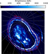 |
Fig. A.1 Exemplar map of UV brightness for PJ11-N. Manually designated features in the outer emission have been highlighted in red. |
In order to determine the location of potential injection signatures in maps of the aurora, an algorithm was developed that combines manual feature designations with an automatic random-forest classifier. This combines the accuracy of manual designation of which features constitute probable injection signatures with the objectivity of the automatic randomforest classifier. A random-forest classifier is a classification model that uses a large number of decision trees to assign labels to data points (Ho 1998). Each decision tree is trained on a random subset of the data and assigns a label to each data point by taking the most common result from the ensemble of decision trees (a ‘forest’). The total number of decision trees in the forest and their length (number of branches or decisions in the tree) can be varied to produce labellings of varying accuracy to the original labels. Random-forest classifiers can be applied to assign labels to unseen data in a partially labelled dataset or, as is the case in this work, to improve the objectivity of a set of manual labels. By varying the number and length of the decision trees in the forest, the ‘coarseness’ of the generated labelling can be modified, from unusably coarse for very small forests of very short trees up to a perfect recreation of the original labelling for very large forests of very tall trees. Somewhere between these two extremes lies a middle ground that will return a labelling that is more objective than the original manual labelling while still approximating it in a broad sense.
Manual labelling of potential injection signatures was performed by designating polygons on maps of the aurora. Since the colour-bar limits of these maps was set at (0, 250) kR, these manual designations are likely insensitive to injection signatures with maximum brightnesses below ~50 kR, though this brightness is comparable with the background brightness of the diffuse aurora and thus injection signatures with this maximum brightness are, in any case, not likely to be easily differentiable from the rest of the aurora. These polygons were designed to comfortably contain the entire injection signature rather than to follow its border exactly, since it was expected that further refinement of the injection-signature masks would be performed by the random-forest classifier. Since these designations were performed ‘by eye’, they are naturally more sensitive to injection signatures that are large in the ionosphere, and thus to regions of weak surface magnetic field. This is not expected to significantly affect the results of this work as Juno performs its perijoves without any bias in subsolar longitude, and hence a particular local time will correspond to many System-III longitudes during the first 40 perijoves.
The random-forest classifier used in this work takes the pixel masks generated by the above manual-designation process and combines them with the pixelwise brightness, colour ratio, and projected radial distance, System-III longitude, and local time in the equatorial magnetosphere to produce automatic pixelwise masks of potential injection signatures. Each data point to be assigned a label by the random-forest classifier is thus a polar-projected-image pixel represented as a vector with five properties. The projected location in the magnetosphere is used alongside the (ionospheric) brightness and colour ratio to refine the behaviour of the detector; the brightness of injection features or the background aurora may vary based on local magnetic-field strength, local time, or distance from the main emission, and so it is important to encode these parameters for the detector. It was a posteriori determined that the random-forest classifier does a very poor job of creating masks for injection signatures when only the brightness and colour ratio are used as inputs. A standard 4:1 train-test split was used to train the classifier and assess its accuracy. A 50-tree forest with tree depth of 100 was determined to adequately perform the classification. Smaller forest sizes or shorter trees gave far less precise injection-signature masks, whereas increasing these parameters above these values, even by orders of magnitude, did not materially alter the performance of the classifier; the results of the 50-tree, 100-depth random-forest classifier represent a settled solution for this dataset. The training of this classifier was performed using the scikit-learn Python package, and resulted in a model accuracy of 97%. Qualitatively, the masks produced by the automatic classifier strongly resemble the manual designations but smoother and more granular. Some injection signatures are split or merged, some are absent, and extra injections have been identified, as expected from an automatic method, but it fundamentally identifies the same population of potential injection signatures as the manual designation. An example of manual designations of potential injection signatures and their automatically determined equivalents is given in Figs. A.1 and A.2. The trained classifier is available for download1.
Appendix B Sensitivity analysis for blob and arc longitudinal extent
It can been seen in Figs. B.1 and B.2 that varying the longitudinal-extent cutoff between automatically detected bloblike and arc-like features in the outer emission by ±10° has little effect on the distribution shown in Fig. 2 (longitudinalextent cutoff = 30°). In all cases, the small-blob features and arc-like features are both concentrated around a projected radial distance of ~11 RJ, with arc-like features being more concentrated in the dusk sector than the noticeably more uniformly distributed small-blob features. The choice of a 30° longitudinalextent cutoff, while chosen as an approximate cutoff between the longitudinal spans of blob-like and arc-like features, is thus not expected to materially affect the conclusions of this work. Indeed, the fact that Figs. B.1 and B.2 show such similar distributions is itself indicative that most blob-like features have longitudinal extents of less than 20°, as assumed by Dumont et al. (2014), and that arc-like features mostly have longitudinal extents of greater than 40°.
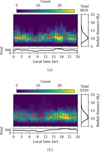 |
Fig. B.1 Histogram in radial distance and local time of the projected position in the equatorial plasma sheet of (a) small blobs and (b) arcs (longitudinal-extent cutoff = 20°) in the outer emission. The meanaverage location for each local-time bin is given by the red line; error bars denote the standard deviation. Histograms flattened in local time and radial distance are given to the bottom and right of the main plot, respectively. |
Appendix C Derivation of scattering surface-field-strength vs. power relation
For the isotropic-scattering case, the precipitating electron flux is controlled by the loss-cone angle α in the ionosphere, which goes as
 (C.1)
(C.1)
where BIS is the magnetic-field strength in the ionosphere and BMS the magnetic-field strength at the source of the scattering in the magnetosphere (Mauk et al. 2017b), or
 (C.2)
(C.2)
since BJS ≫ BMS. If we assume, based on the area subtended by the loss cone for a given loss-cone angle, a power of P ∞ α2, then
 (C.3)
(C.3)
and hence the ratio of power in the northern and southern hemispheres, assuming that injection signatures are conjugate between hemispheres and hence arise from the same location in the magnetosphere,
 (C.4)
(C.4)
or equivalently
 (C.5)
(C.5)
This relation assumes that the variability of the intrinsic ‘intensity’ or the average electron energy of the plasma injection has little effect on the ratio of hemispheric auroral power. Different penetration depths (and hence different absorption profiles) between hemispheres may slightly affect this relation and hence account for some of the scatter in Fig. 5.
Appendix D Effect of sub-corotation on the hemispheric power ratio
Figure 5 shows a large degree of scatter, which we suggest may be partially accounted for by the slight sub-corotation of injections. The north-to-south auroral power ratio of injection signatures is typically greater than one for N→S projections (i.e. where the injection signature is detected in the northern hemisphere and magnetically projected to the south) and less than one for S→N projections. In other words, the emitted power in the detected injection signature is larger than the emitted power in the projection of the injection signature in the other hemisphere. This may be due to the slight sub-corotation of injections, which would mean that, for a given injection signature, the conjugate signature in the other hemisphere would be located slightly ahead or behind the original signature in magnetospheric System-III longitude, since Juno has a hour-scale travel time between hemispheres. To test this hypothesis, we consider a hypothetical injection signature with Gaussian power profile
 (D.1)
(D.1)
where p0 is the peak power, θ is the System-III longitude of a given point, μ is the central longitude, and σ is the RMS width of the injection signature. To calculate the total power, P, of the injection signature, we integrate within a set of reasonable bounds for our detected signature, that we take to be μ ± 2σ, and so
![Mathematical equation: \begin{split} P &= p_{0} \int_{\mu - 2\sigma}^{\mu + 2\sigma} d\theta \cdot \exp \left( -\frac{(\theta - \mu)^2}{2\sigma^2} \right) \\ &= p_{0} \cdot \left[\sqrt{\frac{\pi}{2}} \cdot \sigma \cdot \text{erf} \left( \frac{\mu - \theta}{\sqrt{2}\sigma} \right) \right]_{\mu - 2\sigma}^{\mu + 2\sigma}. \end{split}](/articles/aa/full_html/2026/03/aa58607-25/aa58607-25-eq10.png) (D.2)
(D.2)
For the power contained in the projected injection-signature bounds, Pproj, we assume that the injection signature has moved by θ̇t, where θ̇ is the sub-corotation rate in degrees per hour and t the Juno hemisphere traversal time in hours, and hence
![Mathematical equation: P_{\text{proj}} = p_{0} \cdot \left[\sqrt{\frac{\pi}{2}} \cdot \sigma \cdot \text{erf} \left( \frac{\mu - \theta}{\sqrt{2}\sigma} \right) \right]_{\mu - 2\sigma + \dot{\theta}t}^{\mu + 2\sigma + \dot{\theta}t}.](/articles/aa/full_html/2026/03/aa58607-25/aa58607-25-eq11.png) (D.3)
(D.3)
Since the Gaussian function is symmetrical about its mean, this expression is valid for both N→S and S→N projections, i.e. whether the conjugate injection signature is ahead or behind of its expected (fully corotational) projected location. The ratio of these two powers is thus
![Mathematical equation: \frac{P}{P_{\text{proj}}} = \frac{\left[ \text{erf} \left( \frac{\mu - \theta}{\sqrt{2}\sigma} \right) \right]_{\mu - 2\sigma}^{\mu + 2\sigma}}{\left[ \text{erf} \left( \frac{\mu - \theta}{\sqrt{2}\sigma} \right) \right]_{\mu - 2\sigma + \dot{\theta}t}^{\mu + 2\sigma + \dot{\theta}t}}](/articles/aa/full_html/2026/03/aa58607-25/aa58607-25-eq12.png) (D.4)
(D.4)
or equivalently
 (D.5)
(D.5)
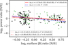 |
Fig. D.1 North-to-south UV auroral power ratio (conjugate area only) vs surface magnetic-field-magnitude ratio for injection signatures detected by Juno-UVS during the first 40 perijoves. The N→S projections are denoted by black ×, and the S→N projections by green +. The best-fit linear relation for all points is given by a solid red line, and separate fitted relations for the N→S and S→N case by dotted and dash-dotted lines, respectively. The theoretical pitch-angle-scattering relation is given by a dashed blue line. |
The average vertical shift between the full linear relation in Fig. 5 and the linear relation for the N→S and S→N cases separately is 0.57±0.1, or equivalently, since Fig. 5 is given in log2 space,
 (D.6)
(D.6)
and hence, by assuming that the Juno hemisphere traversal time t = 3 hr, that injection signatures are approximately of longitudinal width σ = 10°, and solving Eq. (D.5) numerically,
 (D.7)
(D.7)
which is equivalent to a corotation fraction of 85±1%. This is within the 80-to-90% corotation fraction given by Dumont et al. (2018) and hence we suggest that the slight sub-corotation of injection signatures combined with Juno’s hour-scale traversal from the northern to the southern hemisphere may account for a significant proportion of the scatter present in Fig. 5.
To test this hypothesis, a modified version of the analysis of Fig. 5 was performed in which only those injection signatures with a detected conjugate signature in the other hemisphere were used. If the injection-signature polygon projected into the other hemisphere has less than 50% of its area covered by a (presumed conjugate) detected injection signature, it is ignored. Additionally, only the area of the two conjugate injection signatures that maps within the area of the other signature is considered when calculating the total emitted power ratio. In principle, this should greatly reduce the effect of a slight sub-corotation on the emitted power ratio. The results of this analysis are shown in Fig. D.1. There remains some significant scatter in the data; however, the fitted linear relations for the N→S and S→N projections are no longer distinct from the overall linear relation. In other words, the notion that the original detected injection signature always emits more power than its projected conjugate in the other hemisphere (present in Fig. 5) is not present in Fig. D.1. We thus conclude that the slight sub-corotation of injections likely plays a significant role in explaining the distribution of points in Fig. 5, in line with the mathematical argument presented above. It should be noted that injection signatures that are small enough to have no overlap in their detection polygons between hemispheres because of this sub-corotation are necessarily ignored by this analysis. This is expected to correspond to injection signatures less than 15° in longitudinal extent (since a feature moving at 85% of corotation moves ~15° in the ~3 hours between Juno passes of the two hemispheres), which may slightly affect the results in Fig. D.1.
Appendix E Supplementary figures
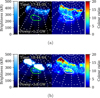 |
Fig. E.1 Injection signature observed on December 11, 2016, at (a) 17:41:35 and (b) 18:44:44 by Juno-UVS during PJ3-S, highlighted in green. The brightness map is given on the left and the colour-ratio map on the right. The main emission is present above the injection signature. |
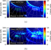 |
Fig. E.2 Injection signature observed on July 11, 2017, at (a) 02:52:48 and (b) 04:21:10 by Juno-UVS during PJ7-S, highlighted in green. The brightness map is given on the left and the colour-ratio map on the right. The main emission is present above the injection signature. |
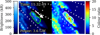 |
Fig. E.3 Injection signature observed at UTC 11:32:49 on April 6, 2019, by Juno-UVS during PJ19-N, highlighted in green. The brightness map is given on the left and the colour-ratio map on the right. The main emission is present to the left of the injection signature. The direction of increasing magnetospheric System-III longitude is indicated by the white arrow. The position of the brightness peak is given by a dotted magenta square in both maps for the sake of comparison. |
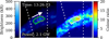 |
Fig. E.4 Injection signature observed at UTC 13:26:13 on April 6, 2019, by Juno-UVS during PJ19-S, highlighted in green. The brightness map is given on the left and the colour-ratio map on the right. The main emission is present below the injection signature. The direction of increasing magnetospheric System-III longitude is indicated by the white arrow. The position of the brightness peak is given by a dotted magenta square in both maps for the sake of comparison. |
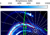 |
Fig. E.5 Juno footprint path (green) overlaid on the exemplar map of the aurora for PJ13-N. An automatically detected arc-type discrete feature crossed by Juno is highlighted in red. The direction of travel of Juno is denoted by the green arrow. |
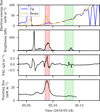 |
Fig. E.6 Juno instrument data for PJ13-N. The crossing of the discrete feature in Fig. E.5 is given in red, and the crossing of the Io footprint tail in green. From top to bottom: JEDI field-aligned (0°-20°, 160°-180°) electron energy flux; UVS footprint brightness; calculated ionospheric field-aligned electrical current; calculated ionospheric Alfvénic Poynt-ing flux. |
All Figures
|
Fig. 1 Exemplar map of UV brightness from PJ7-N, saturated to highlight injection signatures. Automatically detected features in the outer emission have been highlighted according to their feature type as defined in the text: red = small blob (SB), magenta = large blob (LB), green = arc. Gridlines are in jovicentric coordinates and are spaced by 15° in latitude and longitude. |
| In the text | |
|
Fig. 2 Histogram in radial distance and local time of the projected extent in the equatorial plasma sheet of (a) large blobs, (b) small blobs, and (c) arcs in the outer emission. The mean-average location for each local-time bin is given by the red line; error bars denote the standard deviation. Histograms flattened in local time and radial distance are given to the bottom and right of the main plot, respectively. |
| In the text | |
|
Fig. 3 Injection signature observed on May 19, 2017, at (a) 06:51:03 and (b) 07:17:19 by Juno-UVS during PJ6-S, highlighted in green. The brightness map is given on the left and the colour-ratio map on the right. The main emission is present to the right of the injection signature. |
| In the text | |
|
Fig. 4 Histogram in magnetospheric local time of (small and large) blob-like injection features in the outer emission. Features are categorised by the magnetospheric longitude shift between the brightness peak and colour-ratio peak: no shift (<0.5°), slight shift (0.5° to 1°), and shift (>1°), from positive (red, bottom) through to negative (green, top) shifts. |
| In the text | |
|
Fig. 5 North-to-south UV auroral power ratio vs surface magnetic-field-magnitude ratio for injection signatures detected by Juno-UVS during the first 40 perijoves. The N→S projections are denoted by black ×, and the S→N projections by green +. The best-fit linear relation for all points is given by a solid red line, and separate fitted relations for the N→S and S→N case by dotted and dash-dotted lines, respectively. The theoretical pitch-angle-scattering relation is given by a dashed blue line. |
| In the text | |
|
Fig. 6 Juno footprint path (green) overlaid on the exemplar map of the aurora for PJ21-N. An automatically detected small-blob-type discrete feature crossed by Juno is highlighted in red. The direction of travel of Juno is denoted by the green arrow. |
| In the text | |
|
Fig. 7 Juno instrument data for PJ21-N. The crossing of the discrete feature in Fig. 6 is given in red. From top to bottom: JEDI field-aligned (0°-20° upwards, 160°-180° downwards) electron energy flux; UVS footprint brightness; calculated ionospheric field-aligned electrical current; calculated ionospheric Alfvénic Poynting flux. |
| In the text | |
|
Fig. 8 90th-percentile brightness vs 90th-percentile precipitating energy flux based on downward JEDI electrons (25-1000 keV) observed by Juno during crossings of arc-like (blue) and blob-like (red) features in the outer emission. Error bars denote the 80th-100th percentile range. The best-fit linear relation is given by a solid black line, as well as separate best-fit relations for the arc-like (dashed) and blob-like (dash-dotted) features. The theoretical relation after Gérard et al. (2016) is given by the dotted grey line. |
| In the text | |
|
Fig. 9 90th-percentile upward vs downward electron energy flux observed by JEDI during crossings of discrete features in the outer emission. Error bars denote the 80th-100th percentile range. The bestfit linear relation is given by a solid blue line, and the 1:1 relation by a dashed grey line. |
| In the text | |
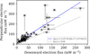 |
Fig. 10 As Fig. 9 but for the downward vs perpendicular electron energy flux. |
| In the text | |
|
Fig. 11 Average electron pitch-angle distribution observed by JEDI during crossings of (a) blob-like and (b) arc-like features in the outer emission. Pitch-angle distributions from individual crossings are given in light grey. 0° (180°) denotes downward (upward) field-aligned electron flux. |
| In the text | |
|
Fig. 12 90th-percentile brightness vs 90th-percentile ionospheric Alfvénic flux extrapolated from Juno(-UVS, -FGM) observations below an altitude of 1 RJ during crossings of arc-like (blue) and blob-like (red) features in the outer emission. Error bars and best-fit relations are denoted as per Fig. 8. |
| In the text | |
|
Fig. 13 90th-percentile brightness vs 90th-percentile upward ionospheric current density extrapolated from Juno(-UVS, -FGM) observations during crossings of discrete features below an altitude of 1 RJ in the outer emission. Error bars denote the 80th-100th percentile range. The best-fit linear relation is given by a solid blue line. |
| In the text | |
|
Fig. A.1 Exemplar map of UV brightness for PJ11-N. Manually designated features in the outer emission have been highlighted in red. |
| In the text | |
 |
Fig. A.2 Same as Fig. A.1 but with automatically detected features. |
| In the text | |
|
Fig. B.1 Histogram in radial distance and local time of the projected position in the equatorial plasma sheet of (a) small blobs and (b) arcs (longitudinal-extent cutoff = 20°) in the outer emission. The meanaverage location for each local-time bin is given by the red line; error bars denote the standard deviation. Histograms flattened in local time and radial distance are given to the bottom and right of the main plot, respectively. |
| In the text | |
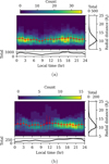 |
Fig. B.2 As Fig. B.1 (a: small blobs, b: arcs) but with a longitudinalextent cutoff of 40°. |
| In the text | |
|
Fig. D.1 North-to-south UV auroral power ratio (conjugate area only) vs surface magnetic-field-magnitude ratio for injection signatures detected by Juno-UVS during the first 40 perijoves. The N→S projections are denoted by black ×, and the S→N projections by green +. The best-fit linear relation for all points is given by a solid red line, and separate fitted relations for the N→S and S→N case by dotted and dash-dotted lines, respectively. The theoretical pitch-angle-scattering relation is given by a dashed blue line. |
| In the text | |
|
Fig. E.1 Injection signature observed on December 11, 2016, at (a) 17:41:35 and (b) 18:44:44 by Juno-UVS during PJ3-S, highlighted in green. The brightness map is given on the left and the colour-ratio map on the right. The main emission is present above the injection signature. |
| In the text | |
|
Fig. E.2 Injection signature observed on July 11, 2017, at (a) 02:52:48 and (b) 04:21:10 by Juno-UVS during PJ7-S, highlighted in green. The brightness map is given on the left and the colour-ratio map on the right. The main emission is present above the injection signature. |
| In the text | |
|
Fig. E.3 Injection signature observed at UTC 11:32:49 on April 6, 2019, by Juno-UVS during PJ19-N, highlighted in green. The brightness map is given on the left and the colour-ratio map on the right. The main emission is present to the left of the injection signature. The direction of increasing magnetospheric System-III longitude is indicated by the white arrow. The position of the brightness peak is given by a dotted magenta square in both maps for the sake of comparison. |
| In the text | |
|
Fig. E.4 Injection signature observed at UTC 13:26:13 on April 6, 2019, by Juno-UVS during PJ19-S, highlighted in green. The brightness map is given on the left and the colour-ratio map on the right. The main emission is present below the injection signature. The direction of increasing magnetospheric System-III longitude is indicated by the white arrow. The position of the brightness peak is given by a dotted magenta square in both maps for the sake of comparison. |
| In the text | |
|
Fig. E.5 Juno footprint path (green) overlaid on the exemplar map of the aurora for PJ13-N. An automatically detected arc-type discrete feature crossed by Juno is highlighted in red. The direction of travel of Juno is denoted by the green arrow. |
| In the text | |
|
Fig. E.6 Juno instrument data for PJ13-N. The crossing of the discrete feature in Fig. E.5 is given in red, and the crossing of the Io footprint tail in green. From top to bottom: JEDI field-aligned (0°-20°, 160°-180°) electron energy flux; UVS footprint brightness; calculated ionospheric field-aligned electrical current; calculated ionospheric Alfvénic Poynt-ing flux. |
| In the text | |
Current usage metrics show cumulative count of Article Views (full-text article views including HTML views, PDF and ePub downloads, according to the available data) and Abstracts Views on Vision4Press platform.
Data correspond to usage on the plateform after 2015. The current usage metrics is available 48-96 hours after online publication and is updated daily on week days.
Initial download of the metrics may take a while.