| Issue |
A&A
Volume 707, March 2026
|
|
|---|---|---|
| Article Number | A328 | |
| Number of page(s) | 15 | |
| Section | Galactic structure, stellar clusters and populations | |
| DOI | https://doi.org/10.1051/0004-6361/202558789 | |
| Published online | 20 March 2026 | |
Abundances in 78 metal-rich bulge spheroid stars from APOGEE
1
Lund Observatory, Department of Geology, Lund University, Sölvegatan 12, Lund, Sweden
2
Nicolaus Copernicus Astronomical Center, Polish Academy of Sciences, ul. Bartycka 18, 00-716 Warsaw, Poland
3
Universidade de São Paulo, IAG, Departamento de Astronomia, 05508-090 São Paulo, Brazil
4
Astrophysikalisches Institut Potsdam, An der Sternwarte 16, Potsdam, 14482, Germany
5
Instituto de Astronomía, Universidad Nacional Autónoma de México, A. P. 106, C.P. 22800, Ensenada, B.C., Mexico
6
Max Planck Institute for Astronomy, Königstuhl 17, 69117 Heidelberg, Germany
7
Instituto de Astrofísica de Canarias, C/ Via Lactea s/n, 38205 La Laguna, Tenerife, Spain
8
Departamento de Astrofísica, Universidad de La Laguna, 38205 La Laguna, Tenerife, Spain
9
Universidad Católica del Norte, Núcleo UCN en Arqueología Galáctica - Inst. de Astronomía, Av. Angamos 0610, Antofagasta, Chile
10
Universidad Católica del Norte, Departamento de Ingeniería de Sistemas y Computación, Av. Angamos 0610, Antofagasta, Chile
★ Corresponding author.
Received:
25
December
2025
Accepted:
9
February
2026
Abstract
Context. The inner Galaxy is the most complex region of the Milky Way, comprising the early bulge, inner thin and thick discs, and inner halo stars; moreover, the formation of the bar caused transfer of gas and stars from the disc to the inner Galaxy. Moreover, accretion of dwarf galaxies took place along the Galaxy’s lifetime, merging with the original bulge. In this work, we sought to constrain the metal-rich stars of the earliest spheroidal bulge.
Aims. With the aim of studying the oldest bulge stars, which show a distribution in a spheroid, we applied a selection based on kinematical and dynamical criteria, in the metal-rich range [Fe/H] >-0.8. This analysis complements our previous work on a symmetric sample with [Fe/H] <-0.8.
Methods. We derived the individual abundances through spectral synthesis for the elements C, N, O, Al, P, S, K, Mn, and Ce using the stellar physical parameters available for our sample from Data Release 17 of the Apache Point Observatory Galactic Evolution Experiment (APOGEE DR17) project in the H band. We also compared the present results, together with literature data, with chemicalevolution models.
Results. The abundances of the alpha elements Mg Si, and Ca, and iron-peak elements V, Cr, Co, and Ni from APOGEE DR17 follow the expected behaviour as compared with the chemical-evolution models. Mn shows the expected secondary behaviour. S and K show a large star-to-star spread, but remain broadly compatible with the model predictions. Phosphorus and cerium display a clear abundance excess around [Fe/H]~ -0.7 that is more pronounced than in our metal-poor sample, suggesting a distinctive chemical signature for the earliest bulge population. Diagnostic diagrams involving [Mg/Mn] versus [Al/Fe] and [Ni/Fe] versus [(C+N)/O] indicate an in situ origin of the bulk of the sample. At super-solar metallicities, a subset of stars shows enhanced K and Mn (and possibly S) together with low [Ce/Fe] ratios, hinting at enrichment processes linked to the nuclear disc and bar. These stars may therefore trace a chemically distinct population shaped by the unique dynamical and star formation conditions of the innermost Galaxy.
Key words: stars: abundances / Galaxy: abundances / Galaxy: bulge / Galaxy: evolution / Galaxy: formation / Galaxy: structure
© The Authors 2026
 Open Access article, published by EDP Sciences, under the terms of the Creative Commons Attribution License (https://creativecommons.org/licenses/by/4.0), which permits unrestricted use, distribution, and reproduction in any medium, provided the original work is properly cited.
This article is published in open access under the Subscribe to Open model. This email address is being protected from spambots. You need JavaScript enabled to view it. to support open access publication.
1 Introduction
The Galactic bulge plays a fundamental role in our understanding of the formation and early evolution of the Milky Way, as it is expected to host a large fraction of the Galaxy’s oldest stellar populations. Its central location, high stellar density, and wide metallicity distribution make the bulge a key laboratory for testing early chemical enrichment and assembly scenarios. Indeed, metallicities of the bulk of the bulge stellar populations span a broad range of approximately -1.5 < [Fe/H] < +0.5 (McWilliam & Rich 1994; Barbuy et al. 2018; Queiroz et al. 2021), reflecting a complex formation history involving rapid early star formation and subsequent dynamical evolution.
Strong age constraints further support the bulge as an ancient Galactic component. The bulk of bulge stars have an estimated age of about 11 Gyr (Clarkson et al. 2008), while the oldest component of, commonly associated with a spheroidal bulge, is inferred to be ~13 Gyr. This is indicated by the ages of bulge globular clusters (GCs) with moderate metallicities (see Table 3 in Souza et al. 2024). These findings are consistent with early formation scenarios in which a significant fraction of the oldest stars in the Galaxy formed rapidly and are now concentrated in the central regions (e.g. Gao et al. 2010; Tumlinson 2010).
We note that at the metal-poor end of the metallicity distribution, the nature of stellar populations in the inner Galaxy becomes increasingly ambiguous. In particular, it is not always clear whether stars with [Fe/H] < -1.5 should be considered bona fide bulge members, part of a metal-poor inner halo, or remnants of accreted systems (e.g. Howes et al. 2016; Geisler et al. 2023; Ardern-Arentsen et al. 2024; Nepal et al. 2026). Despite this ambiguity, metal-poor stars are of exceptional importance, as they are commonly interpreted as tracers of the earliest phases of star formation and chemical enrichment in the Milky Way. Disentangling their origin is therefore both challenging and crucial for reconstructing the bulge’s formation history.
Using a combination of photometric, kinematical, and dynamical diagnostics, Queiroz et al. (2021) identified distinct stellar populations in the inner Galaxy and proposed selection criteria aimed at isolating the spheroidal bulge component. Their analysis showed that these criteria are particularly effective at identifying moderately metal-poor bulge stars, which are often associated with the earliest stellar populations formed in the Milky Way. The identification of the spheroidal bulge is nevertheless difficult, especially given that the bulk of stars in Queiroz et al. (2021) were metal-rich. Building on the selection strategy introduced by Queiroz et al. (2021) and the calculation of stellar orbits, we carried out a series of studies focusing on the chemical properties of the most metal-poor spheroidal bulge candidates, with [Fe/H] < -0.8 (Razera et al. 2022; Barbuy et al. 2023, 2024, 2025a). The abundance patterns of these stars were interpreted in the context of rapid early chemical enrichment.
While metal-poor stars provide a direct window to the earliest bulge formation, extending the analysis to higher metal-licities offers a complementary and necessary perspective. The metal-rich regime may retain chemical signatures of the early bulge while also reflecting later evolutionary processes, and thus it provides an open pathway to understanding the continuity and full metallicity distribution of the spheroidal bulge population. In the present work, we applied the same kinematical and dynamical selection criteria to explore this more metal-rich regime, targeting spheroidal bulge candidates with [Fe/H] > -0.8. This extension allowed us to investigate whether the chemical characteristics identified at lower metallicities persist into the metal-rich tail.
Recent studies have emphasised that particular care is required when interpreting metal-rich bulge samples. In particular, Nepal et al. (2026) identified a spheroidal bulge component with a metallicity distribution function peaking at [Fe/H] ≃ -0.7, but also cautioned that contamination from bar stars on hotter orbits cannot be entirely excluded at the metal-rich end. This highlights the importance of a detailed chemical analysis based on a broad set of elemental abundances, which can provide additional constraints on the nature and origin of these stars beyond kinematical selection alone. Therefore, we selected stars from the reduced proper-motion (RPM) sample of Queiroz et al. (2020, 2021), cross-matched with stars observed in the H band by the Apache Point Observatory Galactic Evolution Experiment (APOGEE; Majewski et al. 2017). We further required effective temperatures of Teff > 3900 K and additional quality control requirements on the spectra, in particular S/N>80. This selection resulted in a sample of 78 stars. For these stars, we analysed the spectra and derived chemical abundances, in particular revising the APOGEE abundances of C, N, O, Al, P, S, K, Mn, and Ce. The abundances of Mg, Si, Ca, V, Cr, Co, and Ni are adopted from the APOGEE Stellar Parameters and Chemical Abundances Pipeline (ASPCAP).
In Sect. 2 the sample is described. In Sect. 3 the analysis is presented. In Sect. 4 the results are reported and chemical evolution models are described. In Sect. 5 the results are compared with chemical evolution models and discussed. Conclusions are drawn in Sect. 6.
2 Data and selection sample
Our sample selection closely follows that described in Razera et al. (2022), with the additional requirement that stars satisfy a metallicity cut of [Fe/H] > -0.8. The criteria adopted to define the sample are as follows:
Azimuthal velocity, Vφ < 0, selecting stars counter-rotating with respect to the bulge rotation.
Non-bar-following orbits.
Metallicity: [Fe/H] > -0.8.
Apogalactic distance: Apo < 4 kpc.
Orbital eccentricity: ecc > 0.7.
The adopted cut in azimuthal velocity (Vφ < 0) is an effective criterion to select stars counter-rotating with respect to the bulge. While stars with low orbital eccentricities (ecc < 0.7) may also belong to the spheroidal component, disc stars are not expected to preferentially populate the Vφ < 0 regime. We therefore imposed an eccentricity cut of ecc > 0.7, acknowledging that this requirement introduces a selection bias. This choice is intended to minimise the inclusion of stars on resonant orbits with ambiguous dynamical origins.
The sample includes dynamical information from the studies by Queiroz et al. (2020, 2021), which combined distances derived with the StarHorse code (Santiago et al. 2016; Queiroz et al. 2018), proper motions in equatorial coordinates (RA, Dec) from Gaia Early Data Release 3 (EDR3; Gaia Collaboration 2021), and radial velocities and chemical abundances from the APOGEE survey. Applying the above selection criteria yields an initial sample of 349 stars. We further refined this sample by requiring effective temperatures of Teff ≥ 3900 K and APOGEE spectra with signal-to-noise ratios (S/Ns) > 80, resulting in a sample of 75 stars. Three stars with S/N < 80 (a18, a20, and a72) were also included because they are of interest due to their [Fe/H] ~ -0.5 permitting a better metallicity coverage; so, the final sample consists of 78 stars.
We note that four stars in the final sample (2M17384300-3904130 = a27, 2M17363449-3926379 = a25, 2M18034066-3002198 = a54, and 2M18075097-3202528 = a68) reported values of VSCATTER in the range of 2-5 km s−1. Such values may indicate the presence of binarity and/or pulsation variability. Interestingly, star a27 is classified as P-rich, while a54 is classified as N-rich, suggesting that their chemical abundance patterns may be related to the observed VSCATTER. The kinematical and dynamical characteristics of the sample stars, including coordinates, proper motions, distance, peri- and apo-Galactic distances, maximum height from the Galactic plane, and eccentricity are given in Table A.1.
In Fig. 1 a Kiel diagram of the sample stars is plotted with the effective temperature and gravity log g from APOGEE-ASPCAP, and compared with the RPM sample of Queiroz et al. (2021). We note that metal-rich red giant branch (RGB) stars are cool, as can be seen through the curved and cooler RGB of metal-rich GCs (e.g. Ortolani et al. 2025).
The APOGEE survey is part of the Sloan Digital Sky Survey IV (SDSS-IV/V; Blanton et al. 2017), offering high resolution (R ~ 22 500) and high S/Ns in the H band (15 14016 940 Â; Wilson et al. 2019) and including about 7 × 10⁵ stars. APOGEE-1 and APOGEE-2 used the 2.5 m Sloan Foundation Telescope at the Apache Point Observatory in New Mexico (Gunn et al. 2006), and the 2.5 m Irénée du Pont Telescope at the Las Campanas Observatory in Chile (Bowen & Vaughan 1973), respectively. Santana et al. (2021) and Beaton et al. (2021) reported the target selection for the Southern and Northern Hemispheres, respectively. The detectors are the H2RG (2048 × 2048) Near-Infrared HgCdTe Detectors with 18μ pixels.
A great advantage of the APOGEE project is the stellar parameter derivation, together with chemical abundances, through a Nelder-Mead algorithm (Nelder & Mead 1965) with a simultaneous fit of the stellar parameter’s effective temperature (Teff), gravity (log g), metallicity ([Fe/H]), and microturbulence velocity (vt), together with the abundances of carbon, nitrogen, and α elements. The ASPCAP pipeline (García Pérez et al. 2016) is based on the FERRE code (Allende Prieto et al. 2006) and the APOGEE line list Smith et al. (2021). In the present work, we use APOGEE DR 17 (Abdurro’uf et al. 2022) uncalibrated (spectroscopic) stellar parameters.
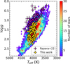 |
Fig. 1 Kiel diagram, based on TEFF_SPEC and LOGG_SPEC from APOGEE DR17 of the present sample, compared to Razera et al. (2022, purple). The RPM sample from Queiroz et al. (2021) is shown in the background as a hexagonally binned density distribution. |
3 Spectroscopic analysis
From our previous work (Razera et al. 2022; Barbuy et al. 2023, 2024, 2025a), we verified that the lines of the following elements were well analysed with the ASPCAP software within the APOGEE collaboration: Mg, Si, Ca, V, Cr, Co, and Ni. In this work, we derived abundances for the elements that are not fully treated with the APOGEE ASPCAP software; they are C, N, O, P, S, K, V, Mn, Ce, and Yb. We also preferred to revise Al. On the other hand, the Na and Ti lines were too blended to be reliable. We derived the abundances in the H band using the TURBOSPECTRUM code from Alvarez & Plez (1998) and Plez (2012) to compute synthetic spectra, which were compared with the observed spectra line-by-line and star-by-star.
The model atmospheres are interpolated within the CN-mild MARCS grids from Gustafsson et al. (2008). The solar abundances of the elements studied are from Asplund et al. (2021).
We adopted the uncalibrated, or ‘spectroscopic’, stellar parameter’s effective temperature (Teff), gravity (log g), metallicity ([Fe/H]), and microturbulence velocity (vt) from the APOGEE DR17 TURBOSPECTRUM results. These parameters are reported in Table 1, together with the S/Ns of the DR17 spectra.
Table 2 reports the lines in the H band that we used to measure the abundances of the elements in the spectra of the sample stars. Oscillator strengths were adopted from the line list of the APOGEE collaboration (Smith et al. 2021). The full atomic line list employed is that from the APOGEE collaboration, together with the molecular lines described in Smith et al. (2021).
Stellar parameters and S/Ns from DR 17.
Line list and oscillator strengths.
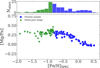 |
Fig. 2 [Mg/Fe] versus [Fe/H] with the histogram of metallicities for the present sample and the Razera et al. (2022) metal-poor sample. |
4 Results
Figure 2 shows the ASPCAP [Mg/Fe] versus [Fe/H] for the sample stars. It is showing the suitability of the sample as an old bulge one and as having a well-covered metallicity range.
4.1 Abundances
In this subsection we describe the derivation of the abundances from the different spectral lines. These are listed below.
C,N,O: for the C, N, O abundance derivation, we used the region 15525-15590 Å, which contains lines of CO, OH, and CN, as described and illustrated in Barbuy et al. (2021) and Razera et al. (2022). The fit is illustrated in Fig. 3 for star a70, where the location of CO, OH, and CN lines are indicated.
Aluminium : Al has three strong and rather clean lines in the H band, located at 16718.957, 16750.539, and 16763.359 Å. The bluest line has a blend in its left wing, and the 16750.539 Å line has two blended lines in its wings that are far enough from the centre to make its abundance reliable. The 16763.359 Å line has a small blend in its left side, as seen in Fig. 4.
Phosphorus : we carried out the fitting of the lines P I 15711.522 Å and P I 16482.932 Å with more weight on the stronger latter line. Only for the more metal-poor stars among the sample were we able to measure a P abundance higher than a solar ratio. In a number of stars, the P measurement is not possible in the spectra where the 16482.932 Å line is too noisy, has strong artefacts, or falls in a gap near the HgCdTe 2048 × 2048 detector edge. Figure 5 illustrates the fit to both P I lines and the nearby CO 15717.2 Å line, which attests the reliability of the strength of a CO feature that coincides with the stronger and more important P I line.
Sulphur : we fitted the three measurable lines: S I 15469.826, 15475.624, and 15478.406 Å. The first two were blended with other atomic and molecular lines; therefore, we derived the S abundances from the third line (see also Hayes et al. 2022; Barbuy et al. 2025a). For the metal-rich stars ([Fe/H]>0), the line is often dominated by other blends and is not very sensitive to the S abundances. Figure 6 shows the fit to the S lines, including the contribution from molecular lines.
Potassium : we simultaneously fitted the two available K I 15163.067 and 15168.376 Å lines, which are plotted in two different panels to better adapt their continua. In most cases, the two lines are well fit with the same K abundance, and in cases where they differ, we adopted a mean value. Figure 7 shows the fit to the K I lines for star a70.
Manganese : The three lines Mn I 15159.200, 15217.793, and 15262.702 Å were measured in all stars. Figure 8 illustrates the fit to the three lines for star a40: 2M17520538-1822315.
Cerium : we simultaneously fitted the six Ce II lines indicated in Table 2. Enhanced Ce was measured in particular for the moderately metal-poor stars with -0.8 < [Fe/H] < -0.7, and this is clear from all six lines. For the metal-rich stars, we relied on the Ce II 16722.51 Å, which is clean, although it is next to another line; the left side of this broad line is a good measure of the Ce abundance. Figure 9 shows the fits for star a15: 2M17263539-2035044, which has [Fe/H]=-0.72 and enhanced Ce.
Ytterbium : the unique Yb line at Yb I 16498.420 Å can only be measured reliably in the warmer and higher S/N spectra. As shown by Montelius et al. (2022), the line itself is blended with CO, but even more difficult is the continuum placement due to the many molecular bands near the Yb line. Due to the low S/N of the spectra in the Yb line region, we do not report their derived abundances.
4.2 Uncertainties
Typical systematic uncertainties due to stellar parameters were evaluated by varying the parameters by fixed amounts of ∆Teff = 100 K, ∆log g = 0.2dex, ∆vt = 0.2 km s−1, shown in Table 3. This was applied to the star a2. Note that the uncertainties in C,N,O are intertwined, as well as the P abundance, which is given by assuming the C,N,O derived for the modified parameters. From Table 3 it is clear that stellar parameters are crucial for having reliable abundances. Fortunately, it appears that the ASPCAP-derived parameters are suitable due to the simultaneous fitting of the parameters plus C,N,O abundances, as discussed in da Silva et al. (2024); however, for stars with over-solar metallicities the errors are larger.
Figure 10 shows the difference between our derived abundances of C, N, O, Al, S, K, Mn, and Ce minus the ones from APOGEE-ASPCAP DR17. The mean difference between the present results and ASPCAP DR17 are given in Eq. (1):
![Mathematical equation: \begin{array}{l}{\rm [C/Fe]}_{\rm present}-{\rm [C/Fe]}_{\rm ASPCAP}=+0.20\\{\rm [N/Fe]}_{\rm present}-{\rm [N/Fe]}_{\rm ASPCAP}=-0.01\\{\rm [O/Fe]}_{\rm present}-{\rm [O/Fe]}_{\rm ASPCAP}=+0.26\\{\rm [Al/Fe]}_{\rm present}-{\rm [Al/Fe]}_{\rm ASPCAP}=-0.13\\{\rm [S/Fe]}_{\rm present}-{\rm [S/Fe]}_{\rm ASPCAP}=-0.03\\{\rm [K/Fe]}_{\rm present}-{\rm [K/Fe]}_{\rm ASPCAP}=+0.03\\{\rm [Mn/Fe]}_{\rm present}-{\rm [Mn/Fe]}_{\rm ASPCAP}=+0.04\\{\rm [Ce/Fe]}_{\rm present}-{\rm [Ce/Fe]}_{\rm ASPCAP}=+0.25.\end{array}](/articles/aa/full_html/2026/03/aa58789-25/aa58789-25-eq1.png) (1)
(1)
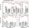 |
Fig. 3 Fit to the 15 525-15 590 Å region in star a70. The main lines are indicated. |
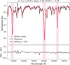 |
Fig. 4 Fit to Al I 16718.957, 16750.539, and 16763.359 Å lines. The synthetic spectra were computed with [Al/Fe] = 0.29 and are shown in red; we compare them with the observed spectrum, which is shown in black. |
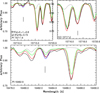 |
Fig. 5 Fit to PI 15711.522 Å and PI 16482.932 Å lines and the nearby CO 15717.2 Å line for star a2: 2M17031887-3421087; this confirms that the CO strength is reliable. Synthetic spectra were computed with [P/Fe] = 0.0 (green), +1.0 (blue), and the final value +0.8 (red), compared with the observed spectrum (black). The dotted line corresponds to molecular lines only. |
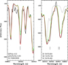 |
Fig. 6 Fit to SI 15469.8036 Å line (left panel) and S I 15475.604, SII 15478.194, and S I 15478.469 Å lines (right panel) for star a35: 2M17463610-2336189. Synthetic spectra were computed with [S/Fe] = 0.0 (green lines), and the final S/Fe] = +0.3 abundance (red lines) is compared with the observed spectrum (black). The dotted black line was computed with molecular lines only. |
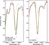 |
Fig. 7 Fit to KI 15163.067 and 15168.376 Å lines for star a70: 2M18084466-2529453. Synthetic spectra were computed with [K/Fe] = 0.0 (green lines); the final value of [K/Fe] = +0.25 (red lines) is compared with the observed spectrum (black). |
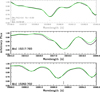 |
Fig. 8 Fit to Mn I 15159.26, 15217.70 and 15262.33 Å lines for star a40: 2M17520538-1822315. Synthetic spectra were computed with [P/Fe] = 0.0 (green lines), and are compared with the observed spectrum (black). |
4.3 Non-LTE effects
For Al, we computed abundances in local thermodynamic equilibrium (LTE) and non-LTE. For that analysis, we computed the synthetic spectra using TURBOSPECTRUM (Gerber et al. 2023), which allowed us to switch from LTE and non-LTE computations using the same code. The non-LTE aluminium calculations were based on the grids presented by Ezzeddine et al. (2018), which provide a prescription for inelastic hydrogen-atom collisions on their 1D non-LTE calculations. The same procedure was applied in Ernandes et al. (2025). It is found that the non-LTE calculation, using TURBOSPECTRUM version 2020 and non-LTE predictions tends to give too-low values of Al. Our Al LTE abundances have a mean value of -0.13, which is lower than the ASPCAP ones (see Eq. (1)). By applying the non-LTE corrections, as available with TURBOSPECTRUM-2020, Al becomes much lower; it is probably maximised non-LTE corrections. As discussed in Ernandes et al. (2025) and Feltzing & Feuillet (2023) based on calculations by Nordlander & Lind (2017), for a giant star a mean correction of -0.2 dex is expected. There are no calculations of non-LTE deviations for the lines of P I, and Ce I analysed in this work; therefore, these uncertainties cannot be evaluated.
For sulphur, Korotin & Kiselev (2024) presented grids of non-LTE corrections for the lines studied here. The corrections range from -0.06 dex for Teff < 4000 K up to about -0.25 dex for Teff ~ 4200 K and [SZFe]=+0.4 to +0.8. The sample stars have rather cool temperatures in the range of 4225 > Teff > 3900 K, where the corrections are not higher than -0.25 dex. Therefore, the non-LTE effects partly explain the S-excesses found for our sample. For K I, the differences between synspec calculations from APOGEE DR17 that take into account non-LTE, and LTE calculations give differences below 0.1 dex.
For manganese, corrections were provided for the lines at 15217.793 and 15262.702 Å by Bergemann & Gehren (2008), but with corrections of 0.1 and 0.5 dex in the mean, respectively. Given this disparity and no available corrections for the third line, we chose not to apply non-LTE corrections to Mn, likewise in Barbuy et al. (2024). Finally, abundances of Mg, Si, Ca, Ti, V, Cr, Co, and Ni adopted from ASPCAP, no non-LTE corrections were applied.
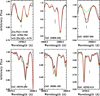 |
Fig. 9 Fit to six Ce lines for star a15: 2M17263539-2035044. Synthetic spectra were computed with [Ce/Fe] = 0.0 (green), and the final value +0.8 (red) is compared with the observed spectrum (black). |
Abundance uncertainties for star a2 due to changes in stellar parameters of ΔTeff = 100 K, Δlog g = 0.2 dex, and Δvt = 0.2 km s−1.
4.4 Chemical-evolution models
The chemical-evolution model first applied to elliptical galaxies (Friaca & Terlevich 1998) is a multi-zone chemical evolution coupled with a hydrodynamical code, allowing the inflow and outflow of gas. The Galactic bulge is assumed to be a classical spheroid with a baryonic mass of 2 × 10⁹ M⊙ and a darkhalo mass of 1.3 × 10¹⁰ M⊙. Cosmological parameters from the Planck Collaboration (2020) were adopted: Ωm = 0.31, ΩΛ = 0.69, a Hubble constant of H0 = 68 km s−1Mpc−1, and an age of the Universe of 13.801 ± 0.024 Gyr.
For the nucleosynthesis yields, we adopted (i) the metallicity-dependent yields from core-collapse supernovae and type II supernovae (SNe II) from Woosley & Weaver (1995) for massive stars, and for low metallicities (Z < 0.01 Z⊙ , or [Fe/H] < -2.5), the yields are from high-explosion-energy hypernovae from Nomoto et al. (2013); (ii) type Ia supernovae (SNe Ia) yields from Iwamoto et al. (1999) - their models W7 (progenitor star of initial metallicity Z = Z⊙) and W70 (zero initial metallicity); and (iii) yields from van den Hoek & Groenewegen (1997) with variable η (the asymptotic giant branch case) for intermediate-mass stars (0.8-8 M⊙) with initial Z = 0.001, 0.004, 0.008, 0.02, and 0.4. For the metal-poor stars, neutrino-interaction processes were also considered, adopting yields from Yoshida et al. (2008). For more details, see Barbuy et al. (2025a).
Corrections to yields from WW95 follow recommendations from Timmes et al. (1995); these are a factor-of-two multiplication for Co and P, and a factor of up to four for K measurements (see more details in Barbuy et al. 2024, 2025a). Models were computed for radii of r < 0.5, 0.5 < r < 1, 1 < r < 2, and 2 < r < 3 kpc from the Galactic centre and for specific star-formation rate values of ν = 1 and 3 Gyr−1. The final abundances are reported in Table A.1.
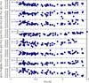 |
Fig. 10 [C, N, O, Al, S, K, MN, Ce/Fe] versus [Fe/H], plotting the differences between the present results and the APOGEE DR17 values. Error bars correspond to the errors for the cool star reported in Table 3. |
5 Discussion
Figure 11 shows the fit to the alpha elements Mg, Si, and Ca, which were derived in the ASPCAP procedure both for the present sample and the metal-poor spheroid sample described in Razera et al. (2022). For these elements, the lines are clean and the ASPCAP results are fully reliable, although for Si there is a non-negligible spread on the metal-poor side. Our chemical evolution model was applied to these alpha elements in Razera et al. (2022), and they were adopted here. The behaviour of these alpha elements is as expected from an old stellar population enriched by SNe II, where the lowering values of the [alpha/Fe] elements is due to the enrichment in Fe by SNe Ia over time; these have a time lag relative to the earliest chemical enrichment by massive stars. The chemical-evolution models form the bulk of the bulge in about 1-0.3 Gyr, showing the abundance ratios of alpha elements to be compatible with a fast chemical enrichment. Note that the more metal-rich stars (from [Fe/H] ≃ -0.7 onwards) appear to require models with higher star-formation efficiency to reproduce the Mg/Fe and Si/Fe ratios, whereas for Ca the same models over-predict the Ca/Fe ratios for metallicities larger than [Fe/H] ≃ -0.4.
Further evidence of alpha elements is shown in Fig. 12, which illustrates the magnesium excess relative to calcium in the metal-poor stars. Mg abundance is higher as a consequence of it being formed in the hydrostatic phases of massive stars, while calcium is produced in the explosive phases of the SNe II and SNe Ia (e.g. McWilliam 2016).
In Fig. 13, we plot the present results for [Al/Fe], compared with literature values, and those for chemical-evolution models. The LTE Al abundances fit the chemical-evolution models, whereas the non-LTE results are too low.
The literature data include results from Alves-Brito et al. (2010), Bensby et al. (2017), Johnson et al. (2014), Ryde et al. (2016), Siqueira-Mello et al. (2016), and Barbuy et al. (2023). The different datasets trace a consistent picture and are compatible with model predictions; Al/Fe increases with metallicity, reaches a peak, and then declines as the bulk of SNe Ia contributions to iron set in. The models also predict a substantial scatter at higher metallicities, highlighting the importance of this regime between [Fe/H] -0.8 to solar and beyond when it comes to constraining chemodynamical models of the bulge. The rather high Al abundance at the metal-rich end may be due to metallicity-dependent yields from SNe II (Curtis et al. 2019) and SNe Ia (Bravo 2019; Keegans et al. 2023).
The most interesting result of the present work is the excess abundances of P around the -0.9 ≲ [Fe/H] ≲ -0.6 metallicity range. This effect was already pointed out by Masseron et al. (2020a) and Brauner et al. (2023, 2024), and it was also detected by Barbuy et al. (2025a,b). In Fig. 14 we show the new data compared with values from previous works on the bulge; these include, in particular, our results for bulge stars with [Fe/H] < -0.8, which are complementary to the present data. Also included are stars from moderately metal-rich GCs by Barbuy et al. (2025b). We added the data of Nandakumar et al. (2022) for disc stars because their sample also shows a P excess at the same metallicities of our sample. It confirms that the higher P excesses are found at metallicities of -1.1 < [Fe/H] < -0.5, as already pointed out by Brauner et al. (2023). Here, we found P excess down to [Fe/H] ~ -1.2. We suggest that this is a characteristic of the oldest bulge stars or the inner disc. In Fig. 14, we overplot the chemical-evolution models for specific star-formation rates of ν =1 and 3 Gyr−1 for the phosphorus data. The models were adopted from Barbuy et al. (2025a). It is clear that models assuming standard nucleosynthesis for phosphorus are unable to reproduce the observed P excess, suggesting that this discrepancy may be related to the nature of the stars contributing to the very early phases of bulge enrichment (see discussions in Chiappini et al. 2011 and Barbuy et al. 2018). The evidence showing that it occurs in the limited-metallicity range cited above for our selected sample with characteristics of bulge spheroid stars coincides with the recent identification of the old spheroidal bulge from a large sample of APOGEE and Gaia RVS (Radial Velocity Spectrometer) by Nepal et al. (2026); this sample shows a peak metallicity at [Fe/H] ~ -0.7. The P excess in part of the stars could be seen as an effect of second-generation stars stripped from GCs or, otherwise, due to an early enrichment by massive stars Barbuy et al. (2025b, see discussion).
Figure 14 (middle panel) shows the present sulfur abundances compared with literature data by Lucertini et al. (2022) and Barbuy et al. (2025a). We see an S excess particularly around a metallicity of [Fe/H] ~ -0.7, and the same is found from the ASPCAP results. The non-LTE effects, as computed by Korotin & Kiselev (2024), partly explain this excess.
Figure 14 (lower panel) shows the K abundances for our sample compared with literature data, including those of Barbuy et al. (2025a) and Reinhard & Laird (2024) for halo stars, which we included to show the level of K abundances on the metal-poor side. There is a considerable spread in the K abundances, but it is compatible with the models. The K excess of the two very metalrich and K-rich stars is confirmed, and the spectra cannot be reproduced with the lower ASPCAP K abundances. The yields of 39K are over-estimated by the classic models of SNe II by a (high) factor of ten; following Timmes et al. (1995), we adopted a factor of four for Z≤Z⊙. Ingredients that can increase the yields would be the rotation of massive stars (Limongi & Chieffi 2018) or shell mergers in the late evolution of massive stars (Rauscher et al. 2002; Ritter et al. 2018). In fact, the abundances can inform us of the presence of these processes.
The iron-peak elements V, Cr, Co, and Ni are plotted in Fig. 15. The abundances for the present sample are the results from ASPCAP, which are combined with results from Razera et al. (2022) for the metal-poor spheroid sample. Our chemicalevolution models were presented in Ernandes et al. (2020) and Barbuy et al. (2024), and the same models are over-plotted on the data. The models fit the data very well, except for the metal-rich end of Ni, where the models tend to give higher Ni than observed for [Fe/H] > -0.5. This is due to yields from SNe Ia from Iwamoto et al. (1999), which over-estimated Ni. As commented in Barbuy et al. (2024), the W7 model over-produces 58Ni, the main Ni isotope. We also needed to take into account the impact of the uncertainties of the weak interaction rates on the yields predicted by Chandrasekhar-mass and sub-Chandrasekhar models of SNe Ia (Bravo 2019; Bravo et al. 2019). As an example, for sub-Chandrasekhar SNe Ia, the yields of 58Ni could increase by a factor of two.
For the iron-peak element Mn, in Fig. 16 the abundances are shown after being re-derived in this work for the sample stars; we added the Barbuy et al. (2024) results for the metal-poor sample and compared them with literature results for bulge stars, including the GCs from Ernandes et al. (2018), the metal-rich cluster NGC 6528 from Sobeck et al. (2006), and the relatively metal-poor cluster NGC 6355 from Souza et al. (2023). We also considered bulge field stars (Nandakumar et al. 2024; Lomaeva et al. 2019; Schultheis et al. 2017; Barbuy et al. 2013); McWilliam et al. (2003) data are from the inner galaxy Sagittarius. We note that although the values of Schultheis et al. (2017) are based on the early results from the APOGEE Data Release 13 (DR13), their dataset is still compatible with our new analysis. The models are the same as in Barbuy et al. (2024), and they clearly show the secondary behaviour of Mn. Overall, the models reproduce most of the data well. Interestingly, the most metal-rich stars exhibit an excess in [Mn/Fe] compared to the model predictions, which may indicate that these stars belong to a distinct stellar population and have experienced a different chemical evolution history. In addition, as discussed previously, a similar behaviour was also shown for K, where some of the most metal-rich stars clearly display enhanced values. Some of the over-abundances found here for the most metal-rich stars remind us of those found recently by Ryde et al. (2025) for nuclear stellar disc (NSD) giants and Nandakumar et al. (2025) for stars in an NSD cluster. An interesting feature is the presence of Mn-rich, metal-rich stars. The increase of [Mn/Fe] with [Fe/H] was already shown by McWilliam (2016). A possible explanation is metallicity-dependent yields, similar to those proposed above for Al. This hypothesis was tested, for instance, in Cescutti et al. (2008), which computed chemical-evolution models that explicitly include metallicity-dependent SN Ia yields for Mn.
Another result of interest is the behaviour of Ce abundances, shown in Fig. 17, with enhancements at the same metallicity range as the P enhancements. The correlation with P and the heavy elements of the fifirst peak (Sr, Y, and Zr) and second peak (Ba, La, Ce, and Nd), which are predominantly s elements was suggested by Masseron et al. (2020b). The present results, together with those from Razera et al. (2022), might suggest such a correlation, but with a large spread. For the most-metal rich stars, we find [Ce/Fe] to be below solar; this is again similar to what was found in the NSD by Ryde et al. (2025) and Nandakumar et al. (2025). In other words, the higher values of [Ce/Fe] at [Fe/H] ~ -0.7 appear to be an effect that we also noted with phosphorus, which is typical of the oldest bulge stellar population; this should be further investigated in future studies. The marked decline at the higher metallicities is another striking feature, and it could be explained by the fast star formation rate in the bulge, leading to solar-metallicity stars not having had time to be enriched by asymptotic giant branch stars.
An important verification is given in Fig. 18 displaying the [Mg/Mn] versus [Al/Fe], which indicates the location of the in situ and ex situ stars as well as high-alpha and low-alpha ones. In the present sample, the more metal-rich stars show a low alpha, as expected, even if they were selected to be part of the spheroidal bulge (see also discussion in Nepal et al. 2026). All our stars have [Al/Fe] ≳ 0.0, which is typical of in situ stars. The sample was compared with the loci of the RPM sample by Queiroz et al. (2021), the Gaia-Enceladus-Sausage (Limberg et al. 2022), and Heracles (Horta et al. 2021). All sample stars are in the in situ origin region. As for those showing low-alpha stars, this is expected since they are metal-rich ([Fe/H]≥0.0), as can be seen in Fig. 11. Some of the most metal-rich ones also show large enhancement of Mn (see Fig. 16), further lowering the [Mg/Mn] ratio. The Ni abundances are all [Ni/Fe]≥0.0, therefore once more indicating the in situ origin of the sample stars.
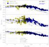 |
Fig. 11 [Mg,Si,Ca/Fe] versus [Fe/H] for bulge spheroid stars. Filled blue pentagons show the ASPCAP results for the present sample; filled yellow pentagons the ASPCAP results for the sample described in Razera et al. (2022). For the chemical-evolution models, different model lines correspond to the outputs of models computed for radii of r < 0.5, 0.5 < r < 1, 1 < r < 2, and 2 < r < 3 kpc from the Galactic centre. Black lines correspond to specific star formation of ν =1 Gyr−1, and blue lines refer to ν =3 Gyr−1. |
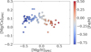 |
Fig. 12 [Mg/Ca] versus [Mg/H] indicating the nucleosynthesis proxies of hydrostatic phases (Mg) compared with a product of explosive phases (Ca). These are colour-coded by their [Fe/H] abundances using the noncalibrated APOGEE DR17 abundances. |
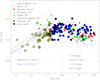 |
Fig. 13 [Al/Fe] versus [Fe/H] for the present results compared with literature bulge samples and chemical evolution models. Blue pentagons refer to this work; four-pointed grey stars to Alves-Brito et al. (2010); filled red circles to Bensby et al. (2017); filled grey triangles and cyan stars to Johnson et al. (2014); filled green circles to Ryde et al. (2016); open grey triangles to Siqueira-Mello et al. (2016); and yellow pentagons to Barbuy et al. (2023). Chemodynamical-evolution models with star formation rate of ν=1 and 3 Gyr−1 or formation timescale of 1 and 0.3 Gyr are over-plotted. |
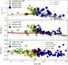 |
Fig. 14 [P/Fe] versus [Fe/H] (upper panel), [S/Fe] versus [Fe/H] (middle panel), and [K/Fe] versus [Fe/H] (lower panel) for the present data compared with literature and chemical evolution models. Blue pentagons show the present results, and yellow pentagons show those of Barbuy et al. (2025a). For P, dark green open stars are for Barbuy et al. (2025b), filled light grey circles for Nandakumar et al. (2022). For S, open forest green squares are for Lucertini et al. (2022). For K, filled green circles show the Reinhard & Laird (2024) results. Different model lines correspond to the outputs of models computed for radii r < 0.5, 0.5 < r < 1, 1 < r < 2, and 2 < r < 3 kpc from the Galactic centre. Black lines correspond to a specific star formation of ν =1 Gyr−1, while red lines show ν = 3 Gyr−1. |
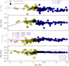 |
Fig. 15 [V, Cr, Co, Ni/Fe] versus [Fe/H] for bulge spheroid stars. Symbols: blue pentagons show ASPCAP results for the present sample, and yellow pentagons show ASPCAP results for the sample described in Razera et al. (2022). Chemical-evolution models Different model lines correspond to the outputs of models computed for radii of r < 0.5, 0.5 < r < 1, 1 < r < 2, and 2 < r < 3 kpc from the Galactic centre. Black lines correspond to a specific star formation of ν =1 Gyr−1, and blue lines show ν = 3 Gyr−1; the red lines are models for ν =1 Gyr−1 and original Co yields from WW95 multiplied by 2. |
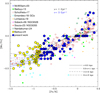 |
Fig. 16 Lower panel: [Mn/Fe] versus [Fe/H]. Chemical-evolution models with star formation rates of ν =1 and 3 Gyr −1 (black and blue lines, respectively) are over-plotted on the results of the present study (blue pentagons) and literature data. Bulge GCs are from Ernandes et al. (2018, blue squares), bulge field stars are from Nandakumar et al. (2024, sea green open stars), Lomaeva et al. (2019, filled orange triangles), Schultheis et al. (2017, open red circles), Barbuy et al. (2013, filled green circles), McWilliam et al. (2003, filled blue triangles), Barbuy et al. (2024, yellow pentagons), and GCs NGC 6528 by Sobeck et al. (2006, filled magenta triangles), NGC 6355 by Souza et al. (2023, filled red triangles). Different model lines correspond to the outputs of models computed for radii r < 0.5, 0.5 < r < 1, 1 < r < 2, and 2 < r < 3 kpc from the Galactic centre. |
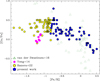 |
Fig. 17 [Ce/Fe] versus [Fe/H] for the present data (open blue stars) compared with literature data: Barbuy et al. (2025a, open red stars), Van der Swaelmen et al. (2016, filled dark green triangles), and Yong et al. (2014, filled magenta pentagons). |
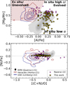 |
Fig. 18 Plotting distribution of our sample stars in the [Mg/Mn] versus [Al/Fe] parameter space, and [Ni/Fe] versus [C+N/O], compared with the loci of the RPM sample and the Heracles and Gaia-Sausage-Enceladus structures. The grey background points show the RPM sample from Queiroz et al. (2021). |
6 Conclusions
We studied bulge sample stars selected from kinematical and dynamical criteria and with a metallicity of [Fe/H] > -0.8, thus completing the work by Razera et al. (2022) and Barbuy et al. (2023, 2024, 2025a) on a symmetric sample with [Fe/H] < -0.8. APOGEE abundances of the alpha elements Mg, Si, and Ca and the iron-peak elements V, Cr, Co, and Ni from the APOGEE-ASPCAP DR17 were adopted, and these elements follow the chemical-evolution models very well.
We re-derived C, N, O, even if the ASPCAP results were reliable, due to the need to have these molecular lines fitted adequately in order to rely on the derivation of the P abundances, for which the unique line is blended with CO. Al abundances were used as indicators of an in situ or ex situ origin of stars. It is important to stress that the indicator is Al in LTE, given that the relative abundances are the reference, as explained in Ernandes et al. (2025). In the present work, essentially all the sample stars show [Al/Fe]≥0.0. S, K, Mn, and Ce were also re-derived, given our previous experience showing that these lines are susceptible to blends or the delicate fitting of profiles.
A first important result is represented by the excesses of P and, possibly, of Ce, with a peak at metallicity [Fe/H]--0.7 to -0.8. This is particularly interesting given that the selection of bulge spheroidal stars by Nepal et al. (2026) shows a metallicity peak exactly at [Fe/H]= -0.7. Therefore, the behaviour of P and Ce might be a particular characteristic of the earliest stellar populations in the Galaxy. S and K show a large spread, but they are compatible with models. For S in particular, non-LTE corrections is rather important.
Finally, the [Mg/Mn] versus [Al/Fe] plot suggested by Hawkins et al. (2015) to be a discriminator between in situ and ex situ stars indicates that our sample appears to have characteristics of an in situ origin. The complementary plot [Ni/Fe] versus [(C+N)/O] (Montalbán et al. 2021; Ortigoza-Urdaneta et al. 2023) also indicates the in situ origin of the sample stars.
Another interesting result, which needs to be confirmed with more data, is related to the most metal-rich stars in our sample. Some of these stars show clear enhancements of K and Mn (and maybe S) and low Ce/Fe ratios. Some of the abundance behaviour observed in the super-solar metallicity regime may be connected to enrichment processes specific to the nuclear disc and the Galactic bar (see discussions in Nepal et al. 2026 and Ryde et al. 2025). In particular, the enhanced abundance ratios seen in the most metal-rich stars could reflect a distinct chemical evolution pathway influenced by the high star-formation efficiency, gas inflows, and bar formation in the innermost regions. If so, these stars may not simply represent the metal-rich extension of inner-disc or bulge populations, but instead trace stellar populations shaped by the unique dynamical and chemical environment of the nuclear disc and bar. Further observational and modelling efforts will be required to disentangle these effects and to assess the relative contributions of different enrichment channels at the highest metallicities.
Acknowledgements
H.E. and S.F. were supported by a project grant from the Knut and Alice Wallenberg Foundation (KAW 2020.0061 Galactic Time Machine, PI Feltzing). B.B., A.C.S.F., and C.C. acknowledge grants from FAPESP, Conselho Nacional de Desenvolvimento Científico e Tecnológico (CNPq) and Coordenaçâo de Aperfeiçoamento de Pessoal de Nivel Superior (CAPES) - Financial code 001. H.E. acknowledges a post-doctoral fellowship at Lund Observatory. S.O.S. acknowledges the support from Dr. Nadine Neumayer’s Lise Meitner grant from the Max Planck Society. A.P.-V., B.B., and S.O.S. acknowledge the DGAPA-PAPIIT grants IA103224 and IN112526 R.P.N. and A.L.R.A. acknowledge the FAPESP Iniciação Científica fellowships no. 2025/05122-1 and 2025/00600-5. BB, HE, PS and SOS are part of the Brazilian Participation Group (BPG) in the Sloan Digital Sky Survey (SDSS), from the Laboratòrio Interinstitucional de e-Astronomia - LIneA, Brazil. J.G.F-T gratefully acknowledges the grants support provided by ANID Fondecyt Postdoc No. 3230001 (Sponsoring researcher), the Joint Committee ESO-Government of Chile under the agreement 2023 ORP 062/2023, and the support of the Doctoral Program in Artificial Intelligence, DISC-UCN. Apogee project: funding for the Sloan Digital Sky Survey IV has been provided by the Alfred P. Sloan Foundation, the U.S. Department of Energy Office of Science, and the Participating Institutions. SDSS acknowledges support and resources from the Center for High-Performance Computing at the University of Utah. The SDSS website is www.sdss.org. SDSS is managed by the Astrophysical Research Consortium for the Participating Institutions of the SDSS Collaboration including the Brazilian Participation Group, the Carnegie Institution for Science, Carnegie Mellon University, Center for Astrophysics I Harvard & Smithsonian (CfA), the Chilean Participation Group, the French Participation Group, Instituto de Astrofísica de Canarias, The Johns Hopkins University, Kavli Institute for the Physics and Mathematics of the Universe (IPMU) / University of Tokyo, the Korean Participation Group, Lawrence Berkeley National Laboratory, Leibniz Institut für Astrophysik Potsdam (AIP), Max-Planck-Institut für Astronomie (MPIA Heidelberg), Max-Planck-Institut für Astrophysik (MPA Garching), Max-Planck-Institut für Extraterrestrische Physik (MPE), National Astronomical Observatories of China, New Mexico State University, New York University, University of Notre Dame, Observatório Nacional / MCTI, The Ohio State University, Pennsylvania State University, Shanghai Astronomical Observatory, United Kingdom Participation Group, Universidad Nacional Autónoma de México, University of Arizona, University of Colorado Boulder, University of Oxford, University of Portsmouth, University of Utah, University of Virginia, University of Washington, University of Wisconsin, Vanderbilt University, and Yale University.
References
- Abdurro’uf, Accetta, K., Aerts, C., et al. 2022, ApJS, 259, 35 [NASA ADS] [CrossRef] [Google Scholar]
- Allende Prieto, C., Beers, T. C., Wilhelm, R., et al. 2006, ApJ, 636, 804 [NASA ADS] [CrossRef] [Google Scholar]
- Alvarez, R., & Plez, B. 1998, A&A, 330, 1109 [NASA ADS] [Google Scholar]
- Alves-Brito, A., Meléndez, J., Asplund, M., Ramírez, I., & Yong, D. 2010, A&A, 513, A35 [NASA ADS] [CrossRef] [EDP Sciences] [Google Scholar]
- Ardern-Arentsen, A., Monari, G., Queiroz, A. B. A., et al. 2024, MNRAS, 530, 3391 [NASA ADS] [CrossRef] [Google Scholar]
- Asplund, M., Amarsi, A. M., & Grevesse, N. 2021, A&A, 653, A141 [NASA ADS] [CrossRef] [EDP Sciences] [Google Scholar]
- Barbuy, B., Hill, V., Zoccali, M., et al. 2013, A&A, 559, A5 [NASA ADS] [CrossRef] [EDP Sciences] [Google Scholar]
- Barbuy, B., Chiappini, C., & Gerhard, O. 2018, ARA&A, 56, 223 [Google Scholar]
- Barbuy, B., Ernandes, H., Souza, S. O., et al. 2021, A&A, 648, A16 [NASA ADS] [CrossRef] [EDP Sciences] [Google Scholar]
- Barbuy, B., Friaça, A. C. S., Ernandes, H., et al. 2023, MNRAS, 526, 2365 [NASA ADS] [CrossRef] [Google Scholar]
- Barbuy, B., Friaça, A. C. S., Ernandes, H., et al. 2024, A&A, 691, A296 [NASA ADS] [CrossRef] [EDP Sciences] [Google Scholar]
- Barbuy, B., Ernandes, H., Friaça, A. C. S., et al. 2025a, A&A, 700, A184 [NASA ADS] [CrossRef] [EDP Sciences] [Google Scholar]
- Barbuy, B., Fernández-Trincado, J. G., Camargo, M. S., et al. 2025b, AJ, 170, 245 [Google Scholar]
- Beaton, R. L., Oelkers, R. J., Hayes, C. R., et al. 2021, AJ, 162, 302 [NASA ADS] [CrossRef] [Google Scholar]
- Bensby, T., Feltzing, S., Gould, A., et al. 2017, A&A, 605, A89 [NASA ADS] [CrossRef] [EDP Sciences] [Google Scholar]
- Bergemann, M., & Gehren, T. 2008, A&A, 492, 823 [NASA ADS] [CrossRef] [EDP Sciences] [Google Scholar]
- Blanton, M. R., Bershady, M. A., Abolfathi, B., et al. 2017, AJ, 154, 28 [Google Scholar]
- Bowen, I. S., & Vaughan, A. H. J. 1973, Appl. Opt., 12, 1430 [Google Scholar]
- Brauner, M., Masseron, T., García-Hernández, D. A., et al. 2023, A&A, 673, A123 [NASA ADS] [CrossRef] [EDP Sciences] [Google Scholar]
- Brauner, M., Pignatari, M., Masseron, T., García-Hernández, D. A., & Lugaro, M. 2024, A&A, 690, A262 [NASA ADS] [CrossRef] [EDP Sciences] [Google Scholar]
- Bravo, E. 2019, A&A, 624, A139 [NASA ADS] [CrossRef] [EDP Sciences] [Google Scholar]
- Bravo, E., Badenes, C., & Martínez-Rodríguez, H. 2019, MNRAS, 482, 4346 [NASA ADS] [CrossRef] [Google Scholar]
- Cescutti, G., Matteucci, F., Lanfranchi, G. A., & McWilliam, A. 2008, A&A, 491, 401 [NASA ADS] [CrossRef] [EDP Sciences] [Google Scholar]
- Chiappini, C., Frischknecht, U., Meynet, G., et al. 2011, Nature, 472, 454 [Google Scholar]
- Clarkson, W., Sahu, K., Anderson, J., et al. 2008, ApJ, 684, 1110 [NASA ADS] [CrossRef] [Google Scholar]
- Curtis, S., Ebinger, K., Fröhlich, C., et al. 2019, ApJ, 870, 2 [Google Scholar]
- da Silva, P., Barbuy, B., Ernandes, H., et al. 2024, A&A, 687, A66 [NASA ADS] [CrossRef] [EDP Sciences] [Google Scholar]
- Ernandes, H., Barbuy, B., Alves-Brito, A., et al. 2018, A&A, 616, A18 [NASA ADS] [CrossRef] [EDP Sciences] [Google Scholar]
- Ernandes, H., Barbuy, B., Friaça, A. C. S., et al. 2020, A&A, 640, A89 [NASA ADS] [CrossRef] [EDP Sciences] [Google Scholar]
- Ernandes, H., Skúladóttir, Á., Feltzing, S., & Feuillet, D. 2025, A&A, 703, A256 [NASA ADS] [CrossRef] [EDP Sciences] [Google Scholar]
- Ezzeddine, R., Merle, T., Plez, B., et al. 2018, A&A, 618, A141 [NASA ADS] [CrossRef] [EDP Sciences] [Google Scholar]
- Feltzing, S., & Feuillet, D. 2023, ApJ, 953, 143 [NASA ADS] [CrossRef] [Google Scholar]
- Friaca, A. C. S., & Terlevich, R. J. 1998, MNRAS, 298, 399 [CrossRef] [Google Scholar]
- Gaia Collaboration (Brown, A. G. A., et al.) 2021, A&A, 649, A1 [NASA ADS] [CrossRef] [EDP Sciences] [Google Scholar]
- Gao, L., Theuns, T., Frenk, C. S., et al. 2010, MNRAS, 403, 1283 [CrossRef] [Google Scholar]
- García Pérez, A. E., Allende Prieto, C., Holtzman, J. A., et al. 2016, AJ, 151, 144 [Google Scholar]
- Geisler, D., Parisi, M. C., Dias, B., et al. 2023, A&A, 669, A115 [NASA ADS] [CrossRef] [EDP Sciences] [Google Scholar]
- Gerber, J. M., Magg, E., Plez, B., et al. 2023, A&A, 669, A43 [NASA ADS] [CrossRef] [EDP Sciences] [Google Scholar]
- Gunn, J. E., Siegmund, W. A., Mannery, E. J., et al. 2006, AJ, 131, 2332 [NASA ADS] [CrossRef] [Google Scholar]
- Gustafsson, B., Edvardsson, B., Eriksson, K., et al. 2008, A&A, 486, 951 [NASA ADS] [CrossRef] [EDP Sciences] [Google Scholar]
- Hawkins, K., Jofré, P., Masseron, T., & Gilmore, G. 2015, MNRAS, 453, 758 [NASA ADS] [CrossRef] [Google Scholar]
- Hayes, C. R., Masseron, T., Sobeck, J., et al. 2022, ApJS, 262, 34 [NASA ADS] [CrossRef] [Google Scholar]
- Horta, D., Schiavon, R. P., Mackereth, J. T., et al. 2021, MNRAS, 500, 1385 [Google Scholar]
- Howes, L. M., Asplund, M., Keller, S. C., et al. 2016, MNRAS, 460, 884 [NASA ADS] [CrossRef] [Google Scholar]
- Iwamoto, K., Brachwitz, F., Nomoto, K., et al. 1999, ApJS, 125, 439 [NASA ADS] [CrossRef] [Google Scholar]
- Johnson, C. I., Rich, R. M., Kobayashi, C., Kunder, A., & Koch, A. 2014, AJ, 148, 67 [Google Scholar]
- Keegans, J. D., Pignatari, M., Stancliffe, R. J., et al. 2023, ApJS, 268, 8 [NASA ADS] [CrossRef] [Google Scholar]
- Korotin, S. A., & Kiselev, K. O. 2024, Astron. Rep., 68, 1159 [Google Scholar]
- Limberg, G., Souza, S. O., Pérez-Villegas, A., et al. 2022, ApJ, 935, 109 [NASA ADS] [CrossRef] [Google Scholar]
- Limongi, M., & Chieffi, A. 2018, ApJS, 237, 13 [NASA ADS] [CrossRef] [Google Scholar]
- Lomaeva, M., Jönsson, H., Ryde, N., Schultheis, M., & Thorsbro, B. 2019, A&A, 625, A141 [NASA ADS] [CrossRef] [EDP Sciences] [Google Scholar]
- Lucertini, F., Monaco, L., Caffau, E., Bonifacio, P., & Mucciarelli, A. 2022, A&A, 657, A29 [NASA ADS] [CrossRef] [EDP Sciences] [Google Scholar]
- Majewski, S. R., Schiavon, R. P., Frinchaboy, P. M., et al. 2017, AJ, 154, 94 [NASA ADS] [CrossRef] [Google Scholar]
- Masseron, T., García-Hernández, D. A., Santoveña, R., et al. 2020a, Nat. Commun., 11, 3759 [Google Scholar]
- Masseron, T., García-Hernández, D. A., Zamora, O., & Manchado, A. 2020b, ApJ, 904, L1 [Google Scholar]
- McWilliam, A. 2016, PASA, 33, e040 [NASA ADS] [CrossRef] [Google Scholar]
- McWilliam, A., & Rich, R. M. 1994, ApJS, 91, 749 [NASA ADS] [CrossRef] [Google Scholar]
- McWilliam, A., Rich, R. M., & Smecker-Hane, T. A. 2003, ApJ, 592, L21 [NASA ADS] [CrossRef] [Google Scholar]
- Montalbán, J., Mackereth, J. T., Miglio, A., et al. 2021, Nat. Astron., 5, 640 [Google Scholar]
- Montelius, M., Forsberg, R., Ryde, N., et al. 2022, A&A, 665, A135 [NASA ADS] [CrossRef] [EDP Sciences] [Google Scholar]
- Nandakumar, G., Ryde, N., Montelius, M., et al. 2022, A&A, 668, A88 [NASA ADS] [CrossRef] [EDP Sciences] [Google Scholar]
- Nandakumar, G., Ryde, N., Mace, G., et al. 2024, ApJ, 964, 96 [NASA ADS] [CrossRef] [Google Scholar]
- Nandakumar, G., Ryde, N., Schultheis, M., et al. 2025, ApJ, 982, L14 [Google Scholar]
- Nelder, J. A., & Mead, H. 1965, Comput. J., 7, 308 [CrossRef] [Google Scholar]
- Nepal, S., Chiappini, C., Pérez-Villegas, A., et al. 2026, https://doi.org/10.1851/8084-6361/202556326 [Google Scholar]
- Nomoto, K., Kobayashi, C., & Tominaga, N. 2013, ARA&A, 51, 457 [CrossRef] [Google Scholar]
- Nordlander, T., & Lind, K. 2017, A&A, 607, A75 [NASA ADS] [CrossRef] [EDP Sciences] [Google Scholar]
- Ortigoza-Urdaneta, M., Vieira, K., Fernández-Trincado, J. G., et al. 2023, A&A, 676, A140 [NASA ADS] [CrossRef] [EDP Sciences] [Google Scholar]
- Ortolani, S., Souza, S. O., Nardiello, D., Barbuy, B., & Bica, E. 2025, A&A, 698, A181 [NASA ADS] [CrossRef] [EDP Sciences] [Google Scholar]
- Planck Collaboration VI. 2020, A&A, 641, A6 [NASA ADS] [CrossRef] [EDP Sciences] [Google Scholar]
- Plez, B. 2012, Turbospectrum: Code for spectral synthesis, Astrophysics Source Code Library [record ascl:1205.004] [Google Scholar]
- Queiroz, A. B. A., Anders, F., Santiago, B. X., et al. 2018, MNRAS, 476, 2556 [Google Scholar]
- Queiroz, A. B. A., Anders, F., Chiappini, C., et al. 2020, A&A, 638, A76 [NASA ADS] [CrossRef] [EDP Sciences] [Google Scholar]
- Queiroz, A. B. A., Chiappini, C., Perez-Villegas, A., et al. 2021, A&A, 656, A156 [NASA ADS] [CrossRef] [EDP Sciences] [Google Scholar]
- Rauscher, T., Heger, A., Hoffman, R. D., & Woosley, S. E. 2002, ApJ, 576, 323 [Google Scholar]
- Razera, R., Barbuy, B., Moura, T. C., et al. 2022, MNRAS, 517, 4590 [CrossRef] [Google Scholar]
- Reinhard, M. V., & Laird, J. B. 2024, AJ, 167, 6 [Google Scholar]
- Ritter, C., Andrassy, R., Côté, B., et al. 2018, MNRAS, 474, L1 [NASA ADS] [CrossRef] [Google Scholar]
- Ryde, N., Schultheis, M., Grieco, V., et al. 2016, AJ, 151, 1 [Google Scholar]
- Ryde, N., Nandakumar, G., Albarracín, R., et al. 2025, A&A, 699, A176 [NASA ADS] [CrossRef] [EDP Sciences] [Google Scholar]
- Santana, F. A., Beaton, R. L., Covey, K. R., et al. 2021, AJ, 162, 303 [NASA ADS] [CrossRef] [Google Scholar]
- Santiago, B. X., Brauer, D. E., Anders, F., et al. 2016, A&A, 585, A42 [NASA ADS] [CrossRef] [EDP Sciences] [Google Scholar]
- Schultheis, M., Rojas-Arriagada, A., García Pérez, A. E., et al. 2017, A&A, 600, A14 [NASA ADS] [CrossRef] [EDP Sciences] [Google Scholar]
- Siqueira-Mello, C., Chiappini, C., Barbuy, B., et al. 2016, A&A, 593, A79 [NASA ADS] [CrossRef] [EDP Sciences] [Google Scholar]
- Smith, V. V., Bizyaev, D., Cunha, K., et al. 2021, AJ, 161, 254 [NASA ADS] [CrossRef] [Google Scholar]
- Sobeck, J. S., Ivans, I.I., Simmerer, J. A., et al. 2006, AJ, 131, 2949 [Google Scholar]
- Souza, S. O., Ernandes, H., Valentini, M., et al. 2023, A&A, 671, A45 [NASA ADS] [CrossRef] [EDP Sciences] [Google Scholar]
- Souza, S. O., Libralato, M., Nardiello, D., et al. 2024, A&A, 690, A37 [NASA ADS] [CrossRef] [EDP Sciences] [Google Scholar]
- Timmes, F. X., Woosley, S. E., & Weaver, T. A. 1995, ApJS, 98, 617 [NASA ADS] [CrossRef] [Google Scholar]
- Tumlinson, J. 2010, ApJ, 708, 1398 [CrossRef] [Google Scholar]
- van den Hoek, L. B., & Groenewegen, M. A. T. 1997, A&AS, 123, 305 [NASA ADS] [CrossRef] [EDP Sciences] [Google Scholar]
- Van der Swaelmen, M., Barbuy, B., Hill, V., et al. 2016, A&A, 586, A1 [NASA ADS] [CrossRef] [EDP Sciences] [Google Scholar]
- Wilson, J. C., Hearty, F. R., Skrutskie, M. F., et al. 2019, PASP, 131, 055001 [NASA ADS] [CrossRef] [Google Scholar]
- Woosley, S. E., & Weaver, T. A. 1995, in American Institute of Physics Conference Series, 327, Nuclei in the Cosmos III, eds. M. Busso, C. M. Raiteri, & R. Gallino (AIP), 365 [Google Scholar]
- Yong, D., Alves Brito, A., Da Costa, G. S., et al. 2014, MNRAS, 439, 2638 [NASA ADS] [CrossRef] [Google Scholar]
- Yoshida, T., Suzuki, T., Chiba, S., et al. 2008, ApJ, 686, 448 [Google Scholar]
Appendix A Coordinates and orbital parameters
We presents the astrometric, kinematic, and orbital properties of the analysed stars. We list Galactic coordinates, distances, proper motions, radial velocities, and the derived orbital parameters used to characterise the spatial distribution and dynamical behaviour of the metal-rich bulge spheroid sample.
Appendix B Derived abundances
We provide the individual chemical abundances derived in this work for all stars in the sample. The table includes the final abundance ratios adopted in the analysis of the abundance trends discussed in this work.
Coordinates, distances from StarHorse from Queiroz et al. (2021), proper motions from Gaia EDR3, radial velocities and orbit parameters from Queiroz et al. (2020, 2021).
Abundances derived in the present work.
All Tables
Abundance uncertainties for star a2 due to changes in stellar parameters of ΔTeff = 100 K, Δlog g = 0.2 dex, and Δvt = 0.2 km s−1.
Coordinates, distances from StarHorse from Queiroz et al. (2021), proper motions from Gaia EDR3, radial velocities and orbit parameters from Queiroz et al. (2020, 2021).
All Figures
|
Fig. 1 Kiel diagram, based on TEFF_SPEC and LOGG_SPEC from APOGEE DR17 of the present sample, compared to Razera et al. (2022, purple). The RPM sample from Queiroz et al. (2021) is shown in the background as a hexagonally binned density distribution. |
| In the text | |
|
Fig. 2 [Mg/Fe] versus [Fe/H] with the histogram of metallicities for the present sample and the Razera et al. (2022) metal-poor sample. |
| In the text | |
|
Fig. 3 Fit to the 15 525-15 590 Å region in star a70. The main lines are indicated. |
| In the text | |
|
Fig. 4 Fit to Al I 16718.957, 16750.539, and 16763.359 Å lines. The synthetic spectra were computed with [Al/Fe] = 0.29 and are shown in red; we compare them with the observed spectrum, which is shown in black. |
| In the text | |
|
Fig. 5 Fit to PI 15711.522 Å and PI 16482.932 Å lines and the nearby CO 15717.2 Å line for star a2: 2M17031887-3421087; this confirms that the CO strength is reliable. Synthetic spectra were computed with [P/Fe] = 0.0 (green), +1.0 (blue), and the final value +0.8 (red), compared with the observed spectrum (black). The dotted line corresponds to molecular lines only. |
| In the text | |
|
Fig. 6 Fit to SI 15469.8036 Å line (left panel) and S I 15475.604, SII 15478.194, and S I 15478.469 Å lines (right panel) for star a35: 2M17463610-2336189. Synthetic spectra were computed with [S/Fe] = 0.0 (green lines), and the final S/Fe] = +0.3 abundance (red lines) is compared with the observed spectrum (black). The dotted black line was computed with molecular lines only. |
| In the text | |
|
Fig. 7 Fit to KI 15163.067 and 15168.376 Å lines for star a70: 2M18084466-2529453. Synthetic spectra were computed with [K/Fe] = 0.0 (green lines); the final value of [K/Fe] = +0.25 (red lines) is compared with the observed spectrum (black). |
| In the text | |
|
Fig. 8 Fit to Mn I 15159.26, 15217.70 and 15262.33 Å lines for star a40: 2M17520538-1822315. Synthetic spectra were computed with [P/Fe] = 0.0 (green lines), and are compared with the observed spectrum (black). |
| In the text | |
|
Fig. 9 Fit to six Ce lines for star a15: 2M17263539-2035044. Synthetic spectra were computed with [Ce/Fe] = 0.0 (green), and the final value +0.8 (red) is compared with the observed spectrum (black). |
| In the text | |
|
Fig. 10 [C, N, O, Al, S, K, MN, Ce/Fe] versus [Fe/H], plotting the differences between the present results and the APOGEE DR17 values. Error bars correspond to the errors for the cool star reported in Table 3. |
| In the text | |
|
Fig. 11 [Mg,Si,Ca/Fe] versus [Fe/H] for bulge spheroid stars. Filled blue pentagons show the ASPCAP results for the present sample; filled yellow pentagons the ASPCAP results for the sample described in Razera et al. (2022). For the chemical-evolution models, different model lines correspond to the outputs of models computed for radii of r < 0.5, 0.5 < r < 1, 1 < r < 2, and 2 < r < 3 kpc from the Galactic centre. Black lines correspond to specific star formation of ν =1 Gyr−1, and blue lines refer to ν =3 Gyr−1. |
| In the text | |
|
Fig. 12 [Mg/Ca] versus [Mg/H] indicating the nucleosynthesis proxies of hydrostatic phases (Mg) compared with a product of explosive phases (Ca). These are colour-coded by their [Fe/H] abundances using the noncalibrated APOGEE DR17 abundances. |
| In the text | |
|
Fig. 13 [Al/Fe] versus [Fe/H] for the present results compared with literature bulge samples and chemical evolution models. Blue pentagons refer to this work; four-pointed grey stars to Alves-Brito et al. (2010); filled red circles to Bensby et al. (2017); filled grey triangles and cyan stars to Johnson et al. (2014); filled green circles to Ryde et al. (2016); open grey triangles to Siqueira-Mello et al. (2016); and yellow pentagons to Barbuy et al. (2023). Chemodynamical-evolution models with star formation rate of ν=1 and 3 Gyr−1 or formation timescale of 1 and 0.3 Gyr are over-plotted. |
| In the text | |
|
Fig. 14 [P/Fe] versus [Fe/H] (upper panel), [S/Fe] versus [Fe/H] (middle panel), and [K/Fe] versus [Fe/H] (lower panel) for the present data compared with literature and chemical evolution models. Blue pentagons show the present results, and yellow pentagons show those of Barbuy et al. (2025a). For P, dark green open stars are for Barbuy et al. (2025b), filled light grey circles for Nandakumar et al. (2022). For S, open forest green squares are for Lucertini et al. (2022). For K, filled green circles show the Reinhard & Laird (2024) results. Different model lines correspond to the outputs of models computed for radii r < 0.5, 0.5 < r < 1, 1 < r < 2, and 2 < r < 3 kpc from the Galactic centre. Black lines correspond to a specific star formation of ν =1 Gyr−1, while red lines show ν = 3 Gyr−1. |
| In the text | |
|
Fig. 15 [V, Cr, Co, Ni/Fe] versus [Fe/H] for bulge spheroid stars. Symbols: blue pentagons show ASPCAP results for the present sample, and yellow pentagons show ASPCAP results for the sample described in Razera et al. (2022). Chemical-evolution models Different model lines correspond to the outputs of models computed for radii of r < 0.5, 0.5 < r < 1, 1 < r < 2, and 2 < r < 3 kpc from the Galactic centre. Black lines correspond to a specific star formation of ν =1 Gyr−1, and blue lines show ν = 3 Gyr−1; the red lines are models for ν =1 Gyr−1 and original Co yields from WW95 multiplied by 2. |
| In the text | |
|
Fig. 16 Lower panel: [Mn/Fe] versus [Fe/H]. Chemical-evolution models with star formation rates of ν =1 and 3 Gyr −1 (black and blue lines, respectively) are over-plotted on the results of the present study (blue pentagons) and literature data. Bulge GCs are from Ernandes et al. (2018, blue squares), bulge field stars are from Nandakumar et al. (2024, sea green open stars), Lomaeva et al. (2019, filled orange triangles), Schultheis et al. (2017, open red circles), Barbuy et al. (2013, filled green circles), McWilliam et al. (2003, filled blue triangles), Barbuy et al. (2024, yellow pentagons), and GCs NGC 6528 by Sobeck et al. (2006, filled magenta triangles), NGC 6355 by Souza et al. (2023, filled red triangles). Different model lines correspond to the outputs of models computed for radii r < 0.5, 0.5 < r < 1, 1 < r < 2, and 2 < r < 3 kpc from the Galactic centre. |
| In the text | |
|
Fig. 17 [Ce/Fe] versus [Fe/H] for the present data (open blue stars) compared with literature data: Barbuy et al. (2025a, open red stars), Van der Swaelmen et al. (2016, filled dark green triangles), and Yong et al. (2014, filled magenta pentagons). |
| In the text | |
|
Fig. 18 Plotting distribution of our sample stars in the [Mg/Mn] versus [Al/Fe] parameter space, and [Ni/Fe] versus [C+N/O], compared with the loci of the RPM sample and the Heracles and Gaia-Sausage-Enceladus structures. The grey background points show the RPM sample from Queiroz et al. (2021). |
| In the text | |
Current usage metrics show cumulative count of Article Views (full-text article views including HTML views, PDF and ePub downloads, according to the available data) and Abstracts Views on Vision4Press platform.
Data correspond to usage on the plateform after 2015. The current usage metrics is available 48-96 hours after online publication and is updated daily on week days.
Initial download of the metrics may take a while.