| Issue |
A&A
Volume 708, April 2026
|
|
|---|---|---|
| Article Number | A149 | |
| Number of page(s) | 12 | |
| Section | Extragalactic astronomy | |
| DOI | https://doi.org/10.1051/0004-6361/202555659 | |
| Published online | 03 April 2026 | |
Identifying lopsidedness in spiral galaxies using a deep convolutional neural network
1
Indian Institute of Science, Education and Research, Tirupati, 517619, India
2
Biswa Bangla Biswabidyalay, Bolpur, 731204, India
3
Indian Institute of Technology, Kharagpur, 721302, India
★ Corresponding author: This email address is being protected from spambots. You need JavaScript enabled to view it.
Received:
26
May
2025
Accepted:
12
January
2026
Abstract
Context. About 30% of disk galaxies exhibit lopsidedness in their stellar disk. Although such a large-scale asymmetry in the disk can be primarily considered as a long-lived mode (m = 1), the physical origin of the lopsidedness in the disk continues to present a puzzling issue.
Aims. In this work, we employ a transfer-learning approach for the automated identification of lopsided galaxies, using SDSS DR18 imaging by fine-tuning a Zoobot model, a deep convolutional neural network (DCNN) package pre-trained on the Galaxy Zoo dataset.
Methods. We obtained 7042 well-resolved, nearly face-on spiral galaxies from SDSS DR18 over the redshift range 0.01 ≤z ≤ 0.1, with an extinction-corrected g-band model magnitude < 16 and Petrosian radius (enclosing 90% of the flux) ≥ 3 arcsec. Of these, we visually identified 490 lopsided and 444 symmetric galaxy samples suitable for training. The trained model achieved a testing accuracy of (87 ± 0.02)%, averaged over ten independent trials.
Results. Using the best-performing model, we identified 3679 lopsided and 2429 symmetric galaxies from the remaining sample. Of these, 2658 lopsided and 1455 symmetric galaxies were predicted with a high level of probability, namely, Ppred ≥ 0.85. The lopsided galaxies in our predicted samples are relatively high star-forming, bluer, low-concentration (late- type), and low-mass galaxies, as compared to the symmetric galaxies.
Conclusions. Our study offers an usable catalogue of lopsided and symmetric galaxies, providing new insights into the formation of lopsidedness in disk galaxies.
Key words: methods: miscellaneous / galaxies: evolution / galaxies: formation / galaxies: kinematics and dynamics / galaxies: spiral / galaxies: structure
© The Authors 2026
 Open Access article, published by EDP Sciences, under the terms of the Creative Commons Attribution License (https://creativecommons.org/licenses/by/4.0), which permits unrestricted use, distribution, and reproduction in any medium, provided the original work is properly cited.
This article is published in open access under the Subscribe to Open model. This email address is being protected from spambots. You need JavaScript enabled to view it. to support open access publication.
1. Introduction
A significant fraction of disk galaxies host large-scale asymmetry in their gas and/or stellar disk. Baldwin et al. (1980) was the first to study the asymmetry in atomic hydrogen (HI) distribution of about 20 spiral galaxies, where half of the distribution appears to be more extended than the other; in fact, he coined the term ‘lopsided’ to indicate this type of asymmetry in the disk. Rix & Zaritsky (1995) considered the NIR observations of 18 face-on spiral galaxies and found that 30% of them are significantly lopsided. They quantified lopsidedness with the m = 1 amplitude in the Fourier decomposition of the surface brightness distribution. The high incidence of lopsidedness in disk galaxies was further confirmed by (i) Zaritsky & Rix (1997), who studied 60 field spiral galaxies; (ii) Bournaud et al. (2005), who studied 149 spiral galaxies in the OSUBGS sample; (iii) Reichard et al. (2008), who investigated lopsidedness in 25 000 nearby galaxies from the SDSS Data Release 4; and (iv) Zaritsky et al. (2013), who studied a sample of 167 galaxies spanning a wide range of morphologies and luminosities, among other properties. van Eymeren et al. (2011) studied the kinematical lopsidedness in a sample of 70 galaxies from the Westerbork H I Survey of Spiral and Irregular Galaxies (WHISP). The ubiquity of these large-scale asymmetries suggests that disk is dynamically unstable against m = 1 perturbation.
Lopsidedness influences the dynamics and secular evolution of the galaxy (see Jog & Combes 2009 for a detailed review). The non-axisymmetric m = 1 mode exerts gravitational torques on the stars, driving the outward transport of angular momentum (Saha & Jog 2014). The possible origin of lopsidedness is either attributed to minor mergers (Zaritsky & Rix 1997), tidal interactions (Kornreich et al. 2002), or flybys (Mapelli et al. 2008). These mechanisms are frequent in denser environments and generate a short-lived (i.e. ∼1–2 Gyr), yet strong lopsided feature in galaxies (Mapelli et al. 2008). Interestingly, there is no correlation between lopsidedness and the strength of the tidal interaction parameter (Bournaud et al. 2005) or the presence of nearby companions (Wilcots & Prescott 2004). Recently, Dolfi et al. (2023) considered lopsided galaxies sample at z = 0 from the IllustrisTNG simulation and showed that regardless of the environment, the internal properties (e.g. the central stellar mass density and disk-to-total mass ratio) play a major role in determining the susceptibility of disk galaxies to such perturbations. The above results were further confirmed for redshifts between 0 < z < 2 by Dolfi et al. (2025). However, these authors observed that at higher redshifts (1.5 < z < 2), environmental factors exert a significant influence on the mechanisms generating lopsidedness. Strong lopsided features are also observed in late-type field galaxies. Bournaud et al. (2005) showed that asymmetric gas accretion via cosmological filaments (leading to asymmetric star formation in the disk) can generate lopsidedness even in isolated galaxies. Saha et al. (2007) demonstrated that a pure exponential stellar disk sustains a global m = 1 mode and the inclusion of self-gravity makes it long-lived. Through analytical studies, it was demonstrated that a distorted dark matter halo potential (Jog 1997, 2000) or a small offset of 350 pc between the centre of dark matter halo and centre of the galactic disk can lead to strong, long-lived lopsidedness in the disk (Prasad & Jog 2017).
Despite all these studies, the key generating mechanism and the survival of lopsidedness in disk galaxies is not well understood, especially with respect to the occurrence of lopsidedness in isolated galaxies. Although the analytical studies mentioned above have been useful in predicting the possible generating mechanism, they rely on linear approximations and require further comparison with simulations. Varela-Lavin et al. (2023) extracted simulated disk galaxies with Milky Way-like mass halos from the IllustrisTNG simulation and showed that lopsidedness correlates more strongly with internal parameters (e.g. the central stellar surface density) than any particular external driving source. Their results also suggest that lopsided galaxies tend to reside in high-spin and often highly distorted DM halos. Rigorous systematic observational studies, coupled with controlled simulations, are required to understand the impact of environment, halo, and intrinsic disk properties on generating lopsidedness. Thus, obtaining a large sample of lopsided galaxies identified from the present and future surveys will contribute towards the understanding their origin and evolution.
With the advent of large volumes of data from the multi-wavelength deep field high-resolution surveys, visually classifying the morphologies of galaxies through the manual inspection of images becomes a laborious task. Further, the high-resolution survey revealed many new interesting features in the morphology, which demanded a more refined morphological classification system. The citizen science Galaxy Zoo 2 (GZ2) project introduced a visual morphological classification for more than 300 000, wherein volunteers classified galaxies by answering a series of questions based on galaxy images (Willett et al. 2013). The GZ2 project resulted in the detailed morphological classification of the largest and brightest SDSS galaxies. However, with the huge volume of images from future surveys such as the Rubin Observatory Legacy Survey of Space and Time (LSST, Ivezić et al. 2019) and the ESA Euclid space mission (Euclid Collaboration: Mellier et al. 2025), morphological classifications using citizen science project would be impracticable, calling for alternative automated methods for speeding up the process.
Automated approaches using traditional machine learning or the deep learning algorithms are well-established astronomical research tools used for various astronomical studies. There are several applications of ML techniques in different astrophysical problems such as star galaxy classifications, detections of galaxy mergers, finding strong gravitational lenses, predicting the photometric redshift of galaxies, etc. Banerji et al. (2010) utilised the SDSS data and Galaxy Zoo labels for three classes to train an artificial neural network (ANN). The trained network is able to reproduce the human classification in GZ project up to the accuracy of 90%. Deep convolutional neural networks (DCNNs) have significantly improved the process of morphological classification of galaxies thanks to their ability to learn complex patterns from the raw images. Dieleman et al. (2015) used a DCNN trained on Galaxy Zoo datasets and obtained the morphological classification of 55 000 galaxies. Abraham et al. (2018) used a CNN to produce a catalogue of 25 781 barred galaxies from the SDSS DR13 database. Prakash et al. (2020) used DCNNs in determining the fundamental parameters governing the dynamical modelling of interacting galaxy pairs. Sarkar et al. (2023) developed a DCNN to classify spiral galaxies into grand-designs with prominent spiral features and flocculents with fragmented spiral features. Savchenko et al. (2024) applied their trained DCNN to prepare a catalogue of edge-on galaxies based on the data from the Panoramic Survey Telescope and Rapid Response System (Pan-STARRS, Kaiser et al. 2010). Recently, Fontirroig et al. (2025) trained a random forest classifier on the lopsided and symmetric galaxies from the IllustrisTNG simulation and achieved an accuracy of ∼80%.
In this study, we fine-tuned a Zoobot (Walmsley et al. 2023) model based on ConvNeXT_nano, a deep learning Python package pre-trained on Galaxy Zoo dataset, for the purpose of identifying lopsided spiral galaxies. The network was trained on the lopsided and symmetric spiral galaxies identified from the SDSS DR18 database. The trained model was then employed to identify a separate larger set of lopsided spiral galaxies from SDSS DR18. We then used this larger sample of lopsided galaxies to study the distribution of their physical properties, such as the specific star formation rate (sSFR), g − i colour, stellar mass, and concentration index. Finally, we addressed the dependence of the performance of the trained model on photometric parameters of galaxies such as redshift and different spiral morphologies. The paper is organised as follows. We describe the selection criteria for the model training dataset in Sect. 2 and the DCNN architecture used in this study in Sect. 3. We present the results in Sect. 4. We present the discussion in Sect. 5 and the conclusions in Sect. 6.
2. Sample
2.1. Sample selection
In this study, we selected nearly face-on spiral galaxies from the SDSS Data Release 18 (DR 18), which provides both photometric and spectroscopic information for the galaxies (Almeida et al. 2023). To build our sample, we started by selecting all primary photometric objects in SDSS DR18 that have been classified as ‘galaxies’ (TYPE flag equal to 3) with the spectroscopic redshifts in the range 0.01 < z < 0.1 and further constraining the sample to an extinction-corrected g-band model magnitude modelMag_g < 16 and Petrosian radius (enclosing 90% of the flux) petroR90_g ≥3 arcsec. This left us with a sample of 29 657 galaxies that are sufficiently resolved and also eliminates contaminating foreground objects. The above choice of constraints is motivated with other previous studies aimed at morphological classification (Nair & Abraham 2010; Willett et al. 2013; Abraham et al. 2025). Next, to extract a subsample of spiral galaxies out of 29 657 galaxies, we utilised the SDSS parameter fracDeV_g. In the SDSS pipeline, the surface brightness distribution for each galaxy is typically fitted using a de Vaucouleurs profile and an exponential profile, while the best-fitting linear combination of both the profile is used to model the distribution. Here, fracDeV_g represents the fraction of luminosity contributed by the de Vaucouleurs profile and it is constrained to lie between 0 and 1. The smaller value of fracDeV_g indicates a disc-dominated profile (late-type), while a higher value represents either a bulge-dominated disc or an elliptical galaxy (early-type). Although various studies have adopted different thresholds to separate between the late-type and early-type galaxies, we used fracDeV_g ≤0.5 (as adopted by Shao et al. 2007 in their studies of late type spirals) to select disc-dominated galaxies. This criteria leaves us with 10 528 galaxies that are dominated by exponential profile. We further restricted our sample using the condition expAB_g ≥0.60 to select nearly face-on galaxies because it is difficult to identify lopsidedness for the highly inclined galaxies. The SDSS parameter expAB_g denotes the axial ratio B/A with A and B as the semi-major and semi-minor axes, respectively. Finally, we were left with a sample of 5557 nearly face-on galaxies. We downloaded RGB cutouts from the SDSS DR18 in jpeg format with a size of 256 × 256 pixels.
Finally, we also considered spiral galaxies which have fracDeV_g > 0.5 with an additional constraint based on the debiased vote fraction from the Galaxy Zoo 2 (GZ2) project for the galaxy to have spiral structure (t04_spiral_a08_spiral_debiased) to be greater than 0.6. These criteria leave us with an additional sample of 2336 candidates for nearly face-on spirals. Upon visual inspection based on the above set of 2336 galaxies, we extracted a reliable set of 1485 face-on spirals, while remaining (595) were discarded for either not being face-on or being mis-classified as spirals based on GZ2 voting criteria. In total, we obtained a sample of 7042 ( = 5557 + 1485) nearly face-on spiral galaxies. Out of these 7042, we selected a sub-sample of galaxies for training a DCNN for the task of binary classification (lopsided and symmetric). The trained DCNN was then utilised for an automatic classification on the remaining samples. We note that although the parameter fracDeV_g has been used in previous studies to select spiral galaxies (imposing a constraint on fracDeV_g, while yielding a sample largely dominated by spirals), it might still admit a small fraction of early-type galaxies. We did not visually inspect the entire sample to exclude such cases. However, when we visually assessed lopsidedness to construct the training sample, we included pure spirals to minimise any contamination from non-spirals in our training set, as detailed in Sect. 2.2.
2.2. Training data
Since DCNNs are supervised machine learning algorithms, the training data must be labelled. As there is currently no large, publicly available catalogue of galaxies classified as lopsided or symmetric, we began by preparing a suitable training sample by annotating a subset from the above extracted nearly face-on spirals as either lopsided or symmetric. Visually, lopsidedness can be identified in face-on images when one side of the disk appears more extended than the other or when the geometric centre does not coincide with the photometric centre. However, visually inspecting a large sample of 7042 galaxies to identify lopsidedness is both unfeasible and prone to introducing bias. Therefore, we randomly selected a smaller, more manageable subset for our training sample. To ensure a representative sampling across redshift, we divided the total redshift range (z = 0.01 − 0.1) into four equal intervals, selecting approximately the same number of galaxies (∼250) from each bin. We chose redshift as the criterion for sampling because it is directly related to the effective resolution of the images (which are later used for the training). Generally, this approach helps minimise potential biases arising from resolution differences. Table 1 lists the total number of galaxies in the parent sample for each redshift bin, along with the number and fraction (relative to the parent sample in each bin) included in the training set. Next, to preserve the quality of the training data, we exclude some ambiguous cases with uncertain classification labels. This process yields a total of 934 galaxies, comprising 490 classified as lopsided and 444 as symmetric. Although this number is relatively small for conventional machine learning models trained from random weight initialisation, it is considered optimal for effectively fine-tuning a domain-specific pretrained model (Walmsley et al. 2023).
Number of galaxies in the parent sample and in the derived training set, binned by redshift.
Quantifying the degree of lopsidedness: Besides the visual inspection, we quantified lopsidedness for the training sample. Lopsidedness is generally quantified by the normalised amplitude of the first mode (m = 1) in the Fourier decomposition of the surface brightness distribution, I, of a galaxy (Rix & Zaritsky 1995). To perform the Fourier decomposition, we divided a galaxy image into concentric circular annuli, centred at the galaxy centre, and performed azimuthal Fourier series decomposition of the surface brightness I in each annulus according to the expression,
![Mathematical equation: $$ \begin{aligned} I (r_k, \phi ) = a_0 (r_k) + \sum ^{m_{\rm max}}_{m = 1} \Big [ a_{m} (r_k) \cos (m (\phi - \phi _m(r_k)) + b_{m} (r_k) \sin (m (\phi -\phi _m(r_k)) \Big ] . \end{aligned} $$](/articles/aa/full_html/2026/04/aa55659-25/aa55659-25-eq1.gif) (1)
(1)
where, am(rk),bm(rk) represents the amplitude for the mode m corresponding to the kth circular annulus (at radius rk) and ϕm(rk) denotes the phase. The normalised value of m = 1 mode amplitude A1(rk) is obtained by dividing  by the zeroth mode a0(rk), i.e., the mean surface brightness. A1(rk) is the value of lopsidedness for the kth circular annulus and when it is averaged within some chosen radial range within the galaxy, it gives the value of lopsidedness, A1, for the galaxy.
Using the astroquery.skyview() module, we downloaded i-band (7480 Å) FITS images (1000 × 1000 pixels) for 934 galaxies from SDSS DR18. We chose the i band to trace the old stellar population. However, we note that value of A1 does not vary significantly across the SDSS g, r, and i-bands (Reichard et al. 2008). Next, the sky backgrounds were determined using the SEP (Barbary 2018) implementation of the SExtractor package (Bertin & Arnouts 1996) and the mean background is subtracted from each image. The foreground stars are also detected using SEP and the regions were masked by interpolating with the pixel values chosen from nearby regions. Although the FITS files are downloaded with the target galaxy approximately centred, accurately determining the photometric centre is crucial for computing A1. Even a shift of 0.5 pixels can significantly affect the measured A1 value (Reichard et al. 2008). We followed the procedure described in Reichard et al. (2008) to refine the galaxy centre and compute A1. The centre is determined starting from the brightest pixel to be the initial estimate and then further improved by computing the first moment of light in a 3 × 3 pixel box centred around the brightest point. Next, we considered the logarithmically spaced radial bins between the Petrosian radius containing 50% and 90% of the Petrosian flux in the i band (R50 and R90, respectively), thereby obtaining a series of circular annuli centred on the refined galaxy centre. In each annulus, we performed a Fourier decomposition of the surface brightness distribution, I, by fitting Eq. (1) (up to the fifth order, m = 5) using a least-squares approach. The fitting gives us different mode amplitudes am(rk),bm(rk) and a phase angle of ϕm(rk) (m = 0–5). The errors associated are derived from the diagonal elements of the covariance matrix. Finally, A1 is computed as the weighted average of the normalised m = 1 amplitude ( ) between R50 and R90, where the weights correspond to the error in each annulus. The median A1 value for lopsided galaxies in the training set is
  , while that for symmetric galaxies is
  , where the superscripts (subscripts) represent the difference between the third (first) quartile and the median value. Since the computation of A1 is subject to systematic uncertainties arising from several steps in the pre-processing and computation processes (most notably the uncertainty in determining the galaxy’s centre) and because there is no well-established threshold of A1 that separates lopsided from symmetric galaxies, we preferred to use the annotations obtained from the visual inspection as more reliable labels for training the DCNN. Figure 1 represents the distribution for redshift, Petrosian radius (enclosing 90% of the flux), extinction-corrected g-magnitude and computed A1 for the lopsided and symmetric galaxies in the training set. Figure 2 presents a subset of galaxy images from the training set. The complete dataset used for training the model is publicly accessible on GitHub1.
 |
Fig. 1. Distributions of redshift, Petrosian radius (enclosing 90% of the flux) in the g-band, extinction-corrected g-band model magnitude modelMag_g, and A1 for the samples of lopsided and symmetric spiral galaxies in the training set (shown from left to right). A few galaxies were excluded from the Petrosian radius and A1 plots to avoid excessive scaling. |
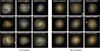 |
Fig. 2. Sub-set of the lopsided (left) and symmetric (right) galaxies from the SDSS DR18 that are used for the training. |
3. Zoobot
Zoobot is a publicly available deep-learning based python package by Walmsley et al. (2023), trained for the morphological classification problems of galaxies. It has been trained on the Galaxy Zoo (GZ) Evo dataset2, which contains about ∼820 k galaxy images from DECaLS/DESI, HST and SDSS. The labels are based on the responses of GZ citizen science projects. Detailed description of the various labels in the GZ decision tree can be found in Walmsley et al. (2022). As it is trained to perform diverse classification tasks based on galaxy morphology, Zoobot can easily be adapted (finetuned) to perform any desired new classification task on galaxies with relatively smaller number of labelled images. This makes Zoobot particularly suitable for our problem, because the number of annotated images for lopsided and symmetric galaxies is limited. In contrast, models with randomly initialised weights typically require a much larger training set when trained from scratch. Before training, we split our labelled dataset (comprising 934 galaxies) into training and testing set by the 80:20 ratio. This allowed us to preserve 186 galaxies of both kinds as the test dataset and the remaining 748 galaxies were used for training+validation.
3.1. Image augmentation
The image dataset comprising 748 samples is divided into training and validation subsets following an 80:20 split, with 80% allocated for training and 20% for validation. Some basic image augmentations are applied for training and validation sets to mitigate the limited sample size:
-
rotation in the range −180° to 180°;
-
horizontal and vertical flipping;
-
zoom-in or -out by 10 per cent.
The details of the total number of images before and after augmentation for the training, validation, and testing sample is shown in Table 2. No augmentation was applied to the test set. We note that although data augmentation increases the effective training set size (by a factor of 4.5, here), such strong augmentation has the possibility to introduce biases due to repeated use of the same underlying samples. However, the ability of data augmentation to improve model generalisation is based on the assumption that the applied augmentations introduce meaningful variations through the above set of geometric transformations.
Sample size for training, validation, and testing for both the classes combined.
3.2. Training Zoobot
In this study, we employed the PyTorch implementation of Zoobot (ZooBotV2) based on the ConvNeXT_nano model as the backbone architecture. The feature extracting backbone (known as the ‘base’) with the pre-trained weights is loaded as an encoder from HuggingFace3 using timm. Next, we added a custom head, which takes the feature maps from the encoder as input. The custom head consists of a global average pooling layer, followed by a fully connected dense layer with 128 neurons, a dropout (of 20%), and a ReLU activation function. Finally, the output layer with two neurons (one for each class) was added. During training, we performed a fine-tuning on the last two blocks of the backbone network (keeping the remaining deeper layers frozen) with a learning rate of 10−5 and layer decay = 0.5. The loss after each training epoch is calculated using the binary cross-entropy function and the optimisation was done using the Adam optimiser with a weight decay = 0.05. The training was performed for a maximum of 50 epochs with a training batch size = 64. However, if the validation loss does not decrease for five consecutive epochs, training is halted, as this indicates that the model is no longer learning and further training could lead to over-fitting. The trained model was then used to make predictions on the test set. We used the softmax activation function to convert the class score into probabilities. We conducted ten independent runs using repeated random splits of data into the training+validation and test sets; namely, each split was generated randomly and the training process was repeated for every run. This was done to mitigate any sampling bias associated with a single training and to ensure that a larger portion of the dataset was included in the test set during evaluation. Figure 3 presents the mean accuracy and loss curve for the training and validation data across ten runs, while the shaded region represents the corresponding ±1σ interval. To train the models, we used an NVIDIA RTX A2000 12 GB GPU (62 GB RAM; 24 physical CPU cores). Each trial required approximately 20 minutes of training before early stopping was triggered. The training and evaluation of the models was done using PyTorch (Paszke et al. 2019).
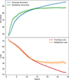 |
Fig. 3. Loss and accuracy of the model as a function of epochs. The solid line represents the mean over ten independent trials, while the shaded band indicates the ±1σ interval. |
3.3. Evaluation performance
The performance of the trained models on the test set is evaluated using several machine-learning metrics, including precision, recall, F1 score, and the receiver operating characteristic (ROC) curves and the corresponding area under the curve (AUC). The ROC curve plots the true positive rate (TPR) against the false positive rate (FPR) across all classification thresholds. The AUC provides a measure of how effectively the classifier distinguishes between the two classes. A perfect classifier yields an AUC of 1, whereas a classifier performing random guessing gives an AUC of 0.5. Figure 4 shows the mean ROC curve obtained from the ten independent trials, with the shaded region indicating the ±1σ interval. For comparison, we have shown the ROC curve for the classifier performing random guessing (AUC = 0.5) as the dashed line. The corresponding mean AUC is 0.94 ± 0.02, demonstrating that the classifier performs robustly across different trials. The mean values (with their ±1σ uncertainties) for the other evaluation metrics across the ten runs are summarised in Table 3. Throughout this study, we adopt the default decision threshold of 0.5 (i.e. if the predicted probability for a class is greater than 0.5, the sample is assigned to that class). The trained models achieves an accuracy of (87 ± 0.02) on the test set for the ten independent trials. Among different trials, we selected the model with the highest AUC (AUC = 0.96, accuracy = 91%) as the representative model for subsequent analysis. The confusion matrix for this selected model is shown in Fig. 5.
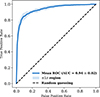 |
Fig. 4. ROC curve. Solid line shows the mean ROC curve for the ten independent trials with the shaded region showing the ±1σ interval. Black dashed line indicates a random-guessing classifier with an AUC of 0.5. |
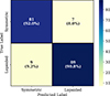 |
Fig. 5. Confusion matrix representing the correctly predicted and falsely predicted sample in the test set, evaluated using the best-performing model (with the greatest testing AUC score). |
Classification report for the test dataset, averaged over ten independent runs with their ±1σ interval.
Visualisation using Grad-CAM: One challenge in assessing the reliability of CNN predictions is the limited understanding of what features the model actually learns during the training. As we move deeper into the network, the learned representations reside in increasingly complex latent spaces and therefore become difficult to interpret without any explainable AI (XAI) techniques. We used one such XAI algorithm known as Gradient-weighted Class Activation Mapping (Grad-CAM; Selvaraju et al. 2019) to visualise the regions of the galaxy images that most strongly influence the model’s predictions. Grad-CAM computes the gradients of the target class score with respect to the feature maps of the final convolutional layer. These gradients are then spatially averaged to obtain importance weights, which quantifies the contribution of each feature map to the target class. Finally, linear combination of the feature maps, weighted by the importance are taken to highlight the regions most relevant for the model prediction. Figure 6 shows examples of galaxy images alongside their corresponding Grad-CAM heat maps overlaid on the original images. The left column of Fig. 6 shows two correctly predicted lopsided galaxies, while the right column presents two correctly predicted symmetric galaxies. In the heat maps, red regions indicate areas of high importance, followed by yellow and green, while blue regions contribute little to the prediction. We observe that when the model correctly predicts a galaxy as lopsided, the red regions in the heat map often tend to be heavily concentrated offset from the centre. In contrast, for symmetric galaxies, the heat map often appears more uniformly distributed throughout the galaxy image. This can be understood as follows: since symmetric galaxies lack distinct asymmetric features, the model assigns roughly equal importance to all regions, resulting in an almost uniform red distribution (right column of Fig. 6) in the heat map. In a few cases, however, the heat maps for symmetric predictions display small patches of high-importance regions that extend beyond the galaxy.
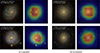 |
Fig. 6. Original images from the test set and the corresponding heat map from the Grad-CAM analysis. The analysis uses the feature maps from the final convolutional layer (just before the global pooling) of the best-performing model to reveal which spatial regions contributed most strongly to the model’s decision-making process (visualised through a heat map where yellow and red regions indicate high importance and blue regions correspond to low importance). The left column shows two correctly predicted lopsided galaxies and the right column presents two correctly predicted symmetric galaxies. In the top-right corner of each image, the probability with which the model would be expected to classify the galaxy as lopsided or symmetric is indicated using the labels pL and pS, respectively. |
4. Results
We used the best-performing model for automatic predictions on the remaining 6108 galaxies (as mentioned in Sect. 2.1). Based on the default prediction probability threshold, Ppred = 0.5, there were 3679 (out of 6108) galaxies predicted to be lopsided and the remaining 2429 were predicted to be symmetric. To ensure a reliable final sample for the statistical study of the physical properties, we chose a threshold of Ppred = 0.85 to represent a high-confidence sample, consisting of 2658 lopsided and 1455 symmetric galaxies. The distribution of redshift for the newly predicted galaxies in the high-confidence sample (Ppred ≥ 0.85) is shown in Fig. 7. We present a sub-set of the newly predicted lopsided and symmetric galaxies sample in Fig. 8. The details of the newly predicted sample, along with the prediction probability for the predicted class, are publicly accessible through our GitHub repository4.
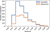 |
Fig. 7. Redshift distributions for the newly predicted galaxy samples, comprising 2658 lopsided and 1455 symmetric systems with prediction probability, Ppred ≥ 0.85. |
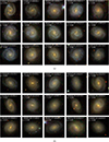 |
Fig. 8. Sub-set of the lopsided (a) and symmetric (b) galaxies predicted from SDSS DR18 using the best-performing model. The prediction probability corresponding to the predicted label is shown at the top-right corner of each image. |
Physical properties: We chose galaxies predicted with Ppred ≥ 0.85 to carry out a statistical study of their physical properties. We used the sSFR and stellar mass (M*) from the SDSS StellarMassFSPSGranWideDust table and Petrosian g - i colour from the SDSS PhotoObj table. We also used the Petrosian radii to obtain the concentration index Ci. Here, Ci = R90/R50 was used as a proxy for the Hubble type, where a higher value of Ci corresponds to an early-type galaxy (Strateva et al. 2001; Shimasaku et al. 2001). In Fig. 9, we show the probability density functions (PDFs) of the sSFR in Gyr−1, g − i colour, log-stellar mass (log(M*/M⊙)) and concentration index (Ci = R90/R50) for the newly predicted samples of lopsided and symmetric spiral galaxies. The median values of the above physical properties of the newly classified sample are presented in Table 4. Additionally, to mitigate any redshift-driven bias arising from the under-representation of symmetric galaxies in our predicted sample at low redshift (z < 0.05; see Fig. 7), we adopted a stratified subsampling approach to ensure equal representation of both categories across the entire redshift range 0.01 ≤ z ≤ 0.1. In the higher redshift range (0.05 ≤ z ≤ 0.1), where the lopsided and symmetric populations have comparable numbers, no sub-sampling was applied and all galaxies are retained. In contrast, the redshift range 0.01 ≤ z < 0.05 shows an imbalance between the two populations. We therefore divided this range into bins of width Δz = 0.01 and, within each bin, randomly sub-sampled the lopsided population, so that its size matches the number of symmetric galaxies (the minority class). This procedure yields a balanced redshift distributions for the lopsided and symmetric samples and the median value of a given physical property can then be computed. To assess the stability of the results against random selection, the sub-sampling procedure was repeated 100 times. The mean of the median values obtained across these 100 realisations is reported in parentheses in Table 4. The standard deviation of the median values across different realisations was found to be negligible and is therefore not explicitly reported.
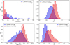 |
Fig. 9. Clockwise from top-left: PDF of the sSFR in Gyr−1, g − i colour, log-stellar mass, log(M*/M⊙), and concentration index, Ci = R90/R50, for the newly predicted samples of lopsided and symmetric spiral galaxies. |
Physical properties for the newly predicted sample.
We find that the lopsided galaxies in our predicted samples are relatively highly star-forming, bluer, low-concentration (late-type), low-mass galaxies. This is consistent with the results from a number of observational and simulation studies (Zaritsky & Rix 1997; Reichard et al. 2008; Łokas 2022). The studies have suggested there is a plausible correlation between lopsidedness in the galaxy and the star formation rate and, hence, an excessive blue luminosity in the galaxy. Lopsidedness in the galaxy arises from the tidal interactions and merger events, which also leads to the inflow of gas in the galaxy and a subsequent increase in the star formation rate. While the origin of lopsidedness typically involves tidal interactions and minor mergers, strong lopsided features are also observed in field galaxies where galaxy interactions are negligible. Bournaud et al. (2005) argued that asymmetric gas accretion, which leads to long-lived lopsidedness in field galaxies, can also result in increased recent star formation activity. The PDF for the log-stellar mass log(M*/M⊙) suggests that lopsided galaxies are low-mass galaxies. This observation is in line with earlier findings (Reichard et al. 2008; Varela-Lavin et al. 2023). The median value of Ci for the lopsided sample is 2.18, while it is 2.55 for the symmetric sample. Kauffmann et al. (2003) showed that Ci = 2.6 can be considered as the approximate threshold separating early-type and late-type galaxies, which suggests that lopsided galaxies generally dominate the late-type population.
5. Discussion
Dependence of model prediction on Redshift: In this study, we have restricted ourselves to bright, low-redshift galaxies because the training sample was built on the basis of visual classification and, during this process, we observed that redshift (connected to image resolution) is a key factor in determining whether a galaxy appears lopsided or symmetric. As redshift increases, the contrast between the brighter and dimmer sides of a galaxy diminishes, causing intrinsically lopsided galaxies to appear more symmetric (Reichard et al. 2008), which may introduce a bias in labelling. To assess the dependence of model performance on redshift, we divided the test sample in different redshift bins and plotted the ROC curve to visualise the model’s performance in each bin across all classification thresholds. The test set was split into four redshift bins: (0.01, 0.03], (0.03, 0.05], (0.05, 0.07], and (0.07, 0.10]. The redshift bins were chosen in such a way that we ended up with approximately equal samples from the test set for each bin. Figure 10a shows the ROC curves for the different redshift bins over the redshift range z = [0.01, 0.1], with the corresponding AUC scores and number of samples, N, for the particular bin indicated in the legend. Comparing the AUC scores allowed us to assess the ability of the model to distinguish between the two classes for different redshift bins. We observed that the model performs fairly well for all redshift bins with AUC > 0.9. However, for the last redshift bin z = (0.07, 0.01], the sample size was small enough for the purposes of a fair comparison.
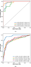 |
Fig. 10. ROC curves for galaxies at different redshift bins, colour-coded as shown in the legend, with each label also listing the corresponding AUC score and the number of galaxies in the bin N. Top Plot (a) shows the ROC curves for different redshift bins within the low redshift range z = [0.01, 0.1] and the bottom plot (b) shows the ROC curves for different redshift bins within the high redshift range z = [0.1, 0.2], along with the ROC curve for the complete low redshift range z = [0.01, 0.1] shown for comparison. |
As a robustness check, we investigated how well the model (trained on low-z samples: z = 0.01 − 0.1) performs at relatively higher z samples. To obtain a representative high-z spiral galaxies from SDSS DR18, we considered the following selection criteria: (i) 0.1 < z < 0.2; (ii) extinction-corrected g-band model magnitude modelMag_g < 18; (iii) Petrosian radius petroR90_g ≥6 arcsec; (iv) fracDeV_g ≤0.5; and (v) expAB_g ≥0.60. These cuts yield 14 312 face-on spiral galaxies for the high-z analysis. To select a representative test sample, we drew samples from different redshift bins. We divided the redshift interval into five equal-width bins. However, due to sparse sampling and reduced visual certainty at the upper end of the redshift range, we merged the last two bins, resulting in the final redshift binning: (0.10, 0.12], (0.12, 0.14], (0.14, 0.16], and (0.16, 0.20]. From each bin, we randomly selected approximately 200 galaxies and visually classified them as lopsided or symmetric to construct a test sample. We then applied our best-performing model to this visually classified set and computed the ROC–AUC score for each redshift bin. Figure 10b presents the ROC curves for different redshift bins within the high-redshift range z = [0.1, 0.2]. For comparison, the ROC curve for the complete low redshift range of z = [0.01, 0.1] is also shown (AUC = 0.96). The model achieves an average AUC score of 0.82 across the high-z bins. Although the AUC score decreases from 0.96 to 0.82 when moving to higher redshift, the model still offers a reasonable capacity to predict correctly at higher redshift. It is also important to note that visual classification becomes challenging at higher redshift, introducing additional bias that may affect the evaluation.
Dependence of model prediction on spiral morphology: In Sect. 4, we show that lopsidedness is more common in late-type spirals (low Ci) with loosely wound arms, whereas symmetric galaxies are more frequently found in early-type spirals (high Ci) with tightly wound arms. Although our goal is to classify galaxies as lopsided or symmetric, it is challenging to completely disentangle this dependence on spiral-arm tightness, as it is intrinsically linked to galaxy morphology. One approach to mitigate this effect is to ensure that the training sample includes sufficient representation of the minor cases; namely, symmetric galaxies with loose winding and lopsided galaxies with tight winding. To confirm this finding, we collected the de Vaucouleurs numerical stage indices (T) from the HyperLeda database (Makarov et al. 2014), which allowed us to identify spiral galaxies based on the tightness of their arm winding. The T values retrieved from the HyperLeda database sometimes show discrepancies with visual morphology; in particular, some early-type spiral galaxies with clearly visible spiral arms are assigned negative T values. As our study is focussed on spiral galaxies, we ensured that the training set (constructed through visual classification) contained only pure spirals. However, it was not feasible to visually inspect the remaining larger sample, which could therefore include a small fraction of non-spiral galaxies. Figure 11 presents the distribution of spiral-arm morphologies for both the training set and the high-confidence predicted sample, where the y-axis represents the percentage of the total sample in each bin. In plotting Fig. 11a, we excluded 18 symmetric and 10 lopsided galaxies from the training set, namely, those whose T values were either unavailable or unreliable. In Fig. 11b, we included only the galaxies with T > 0 from the predicted sample to focus on the relative populations of different spiral-arm morphologies. In terms of winding, we distinguished the T values as follows: (a) tight winding (Sa, Sab): 0 < T < 3; (b) moderate winding (Sb, Sbc): 3 ≤ T < 5; and (c) loose winding (Sc, Scd, Sd, Sm): T ≥ 5. Comparing the relative fractions across winding categories, we find that both lopsided and symmetric galaxies (in both the training and prediction sets) are predominantly moderately wound, followed by loosely wound spirals for lopsided galaxies and tightly wound spirals for symmetric ones. Importantly, the presence of minor cases (i.e., tightly wound lopsided galaxies and loosely wound symmetric galaxies) ensures that the model prediction are not primarily driven by tightness of the spiral arms. Moreover, the GradCAM analysis in Sect. 3.3 further demonstrates that the model successfully captures the relevant morphological features necessary to distinguish between lopsided and symmetric galaxies.
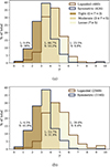 |
Fig. 11. Percentage of various spiral morphologies based on the tightness of the spiral arm winding. The bracketed number indicates the total number in each set. Panel (a): Training set. Panel (b): Prediction set (Ppred ≥ 0.85). The annotated text in the figure shows the percentage of samples for the three different windings. |
Human labelling: Visual inspection was the only preferred method to determine the labels for the training sample. Even though visual inspection of galaxies to identify subtle features such as lopsidedness is time-consuming and requires careful attention, especially in the case of galaxies that lie between the most symmetric and the most lopsided. Excluding those galaxies would result in a significant decline in sample size and also restrict the ability of the model to generalise to a larger sample. Owing to the extreme sensitivity of A1 to various factors (e.g. centre determination), careful visual inspection becomes the only reliable method. To minimise biases introduced during the visual-inspection process, we selected a manageable number of galaxies, repeated the inspection procedure with increased scrutiny, and excluded only those cases for which the classification remained uncertain.
6. Conclusion
We fine-tuned a Zoobot model to identify lopsided spiral galaxies. We selected 7042 nearly face-on spiral galaxies from SDSS DR18 over the redshift range 0.01 ≤ z ≤ 0.1, with extinction-corrected g-band model magnitude modelMag_g < 16 and Petrosian radius (enclosing 90% of the flux) petroR90_g ≥3 arcsec. Due to the non-availability of a sufficiently large sample of galaxies previously classified as lopsided or symmetric, we constructed our training set on the basis of a careful visual inspection. To make the visual classification manageable, we focussed on a relatively smaller subset randomly sampled from the above parent sample, binned across different redshift intervals, resulting in a training sample of 934 galaxies (490 lopsided and 444 symmetric). Next, we fine-tune the Zoobot model based on the ConvNext_nano architecture, achieving a testing accuracy of (87 ± 0.02)%, averaged over ten independent trials. We then used the best-performing model (highest AUC score = 0.96; accuracy = 91%) to make predictions for the remaining 6108 galaxies, identifying 3679 lopsided and 2429 symmetric galaxies. Using the subset of 2658 lopsided and 1455 symmetric galaxies predicted with high probability (Ppred ≥ 0.85), we studied their physical properties. The lopsided galaxies display an excessive blue luminosity, with a higher sSFR, which is in compliance with previous studies. This can be understood by investigating the mechanism which leads to lopsidedness in the disk. For galaxies in denser environments, tidal interactions or minor mergers are the two possible scenarios for generating lopsidedness in the disk, which leads to enhanced star formation. In the field environment where the interactions are less frequent, numerical studies have shown asymmetric gas accretion and a subsequent star formation can create strong lopsidedness in the disk. Hence, even though lopsidedness is a ubiquitous phenomenon observed in both groups or isolated environments, the formation mechanism and the lifetime for the m = 1 mode in galaxies might, in fact, depend on the environment within which the galaxies reside. We also verified the results obtained from the previous studies, asserting that lopsided galaxies have lower concentration index and are less massive compared to symmetric galaxies. Finally, we discuss the dependence of the performance of the trained model on key parameters such as redshift and different spiral morphologies.
Data availability
The dataset and the best-performing model are made publicly available through GitHub at https://github.com/bijusaha-astro/CNN_lopsided.
Acknowledgments
We thank the anonymous referee for their suggestions, which helped to improve the clarity of the paper. We thank Prime Minister’s Research Fellowship (PMRF ID – 0903060) for funding this project. We acknowledge discussions with Dr. Dmitry Makarov and Dr. Sergey Savchenk and we thank them very much for their valuable suggestions. We are also grateful to Prof. Françoise Combes for very useful suggestions during the initial phase of the work. We also thank Mr. Ganesh Narayanan for the useful comments and suggestions. Funding for the Sloan Digital Sky Survey V has been provided by the Alfred P. Sloan Foundation, the Heising-Simons Foundation, the National Science Foundation, and the Participating Institutions. SDSS acknowledges support and resources from the Center for High-Performance Computing at the University of Utah. SDSS telescopes are located at Apache Point Observatory, funded by the Astrophysical Research Consortium and operated by New Mexico State University, and at Las Campanas Observatory, operated by the Carnegie Institution for Science. The SDSS web site is www.sdss.org. SDSS is managed by the Astrophysical Research Consortium for the Participating Institutions of the SDSS Collaboration, including Caltech, The Carnegie Institution for Science, Chilean National Time Allocation Committee (CNTAC) ratified researchers, The Flatiron Institute, the Gotham Participation Group, Harvard University, Heidelberg University, The Johns Hopkins University, L’Ecole polytechnique fédérale de Lausanne (EPFL), Leibniz-Institut für Astrophysik Potsdam (AIP), Max-Planck-Institut für Astronomie (MPIA Heidelberg), Max-Planck-Institut für Extraterrestrische Physik (MPE), Nanjing University, National Astronomical Observatories of China (NAOC), New Mexico State University, The Ohio State University, Pennsylvania State University, Smithsonian Astrophysical Observatory, Space Telescope Science Institute (STScI), the Stellar Astrophysics Participation Group, Universidad Nacional Autónoma de México, University of Arizona, University of Colorado Boulder, University of Illinois at Urbana-Champaign, University of Toronto, University of Utah, University of Virginia, Yale University, and Yunnan University. Software: astropy (Astropy Collaboration 2013, 2018), pytorch (Paszke et al. 2019), seaborn (Waskom et al. 2017).
References
- Abraham, S., Aniyan, A. K., Kembhavi, A. K., Philip, N. S., & Vaghmare, K. 2018, MNRAS, 477, 894 [NASA ADS] [CrossRef] [Google Scholar]
- Abraham, L., Abraham, S., Kembhavi, A. K., et al. 2025, ApJ, 978, 137 [Google Scholar]
- Almeida, A., Anderson, S. F., Argudo-Fernández, M., et al. 2023, ApJS, 267, 44 [NASA ADS] [CrossRef] [Google Scholar]
- Astropy Collaboration (Robitaille, T. P., et al.) 2013, A&A, 558, A33 [NASA ADS] [CrossRef] [EDP Sciences] [Google Scholar]
- Astropy Collaboration (Price-Whelan, A. M., et al.) 2018, AJ, 156, 123 [Google Scholar]
- Baldwin, J. E., Lynden-Bell, D., & Sancisi, R. 1980, MNRAS, 193, 313 [NASA ADS] [CrossRef] [Google Scholar]
- Banerji, M., Lahav, O., Lintott, C. J., et al. 2010, MNRAS, 406, 342 [Google Scholar]
- Barbary, K. 2018, Astrophysics Source Code Library [record ascl:1811.004] [Google Scholar]
- Bertin, E., & Arnouts, S. 1996, A&AS, 117, 393 [NASA ADS] [CrossRef] [EDP Sciences] [Google Scholar]
- Bournaud, F., Combes, F., Jog, C. J., & Puerari, I. 2005, A&A, 438, 507 [NASA ADS] [CrossRef] [EDP Sciences] [Google Scholar]
- Dieleman, S., Willett, K. W., & Dambre, J. 2015, MNRAS, 450, 1441 [NASA ADS] [CrossRef] [Google Scholar]
- Dolfi, A., Gómez, F. A., Monachesi, A., et al. 2023, MNRAS, 526, 567 [NASA ADS] [CrossRef] [Google Scholar]
- Dolfi, A., Gómez, F. A., Monachesi, A., et al. 2025, A&A, 699, A11 [NASA ADS] [CrossRef] [EDP Sciences] [Google Scholar]
- Euclid Collaboration (Mellier, Y., et al.) 2025, A&A, 697, A1 [Google Scholar]
- Fontirroig, V., Gómez, F. A., Arancibia, M. J., Dolfi, A., & Monsalves, N. 2025, A&A, 699, A118 [NASA ADS] [CrossRef] [EDP Sciences] [Google Scholar]
- Ivezić, Ž., Kahn, S. M., Tyson, J. A., et al. 2019, ApJ, 873, 111 [Google Scholar]
- Jog, C. J. 1997, ApJ, 488, 642 [NASA ADS] [CrossRef] [Google Scholar]
- Jog, C. J. 2000, ApJ, 542, 216 [Google Scholar]
- Jog, C. J., & Combes, F. 2009, Phys. Rep., 471, 75 [NASA ADS] [CrossRef] [Google Scholar]
- Kaiser, N., Burgett, W., Chambers, K., et al. 2010, in Ground-Based and Airborne Telescopes III, eds. L. M. Stepp, R. Gilmozzi, & H. J. Hall, SPIE Conf. Ser., 7733, 77330E [Google Scholar]
- Kauffmann, G., Heckman, T. M., White, S. D. M., et al. 2003, MNRAS, 341, 54 [Google Scholar]
- Kornreich, D. A., Lovelace, R. V. E., & Haynes, M. P. 2002, ApJ, 580, 705 [Google Scholar]
- Łokas, E. L. 2022, A&A, 662, A53 [NASA ADS] [CrossRef] [EDP Sciences] [Google Scholar]
- Makarov, D., Prugniel, P., Terekhova, N., Courtois, H., & Vauglin, I. 2014, A&A, 570, A13 [NASA ADS] [CrossRef] [EDP Sciences] [Google Scholar]
- Mapelli, M., Moore, B., & Bland-Hawthorn, J. 2008, MNRAS, 388, 697 [NASA ADS] [CrossRef] [Google Scholar]
- Nair, P. B., & Abraham, R. G. 2010, ApJS, 186, 427 [Google Scholar]
- Paszke, A., Gross, S., Massa, F., et al. 2019, PyTorch: An Imperative Style, High-Performance Deep Learning Library (Red Hook, NY, USA: Curran Associates Inc.) [Google Scholar]
- Prakash, P., Banerjee, A., & Perepu, P. K. 2020, MNRAS, 497, 3323 [Google Scholar]
- Prasad, C., & Jog, C. J. 2017, A&A, 600, A17 [NASA ADS] [CrossRef] [EDP Sciences] [Google Scholar]
- Reichard, T. A., Heckman, T. M., Rudnick, G., Brinchmann, J., & Kauffmann, G. 2008, ApJ, 677, 186 [Google Scholar]
- Rix, H.-W., & Zaritsky, D. 1995, ApJ, 447, 82 [Google Scholar]
- Saha, K., & Jog, C. J. 2014, MNRAS, 444, 352 [Google Scholar]
- Saha, K., Combes, F., & Jog, C. J. 2007, MNRAS, 382, 419 [NASA ADS] [CrossRef] [Google Scholar]
- Sarkar, S., Narayanan, G., Banerjee, A., & Prakash, P. 2023, MNRAS, 518, 1022 [Google Scholar]
- Savchenko, S. S., Makarov, D. I., Antipova, A. V., & Tikhonenko, I. S. 2024, Astron. Comput., 46, 100771 [Google Scholar]
- Selvaraju, R. R., Cogswell, M., Das, A., et al. 2019, Int. J. Comput. Vis., 128, 336 [Google Scholar]
- Shao, Z., Xiao, Q., Shen, S., et al. 2007, ApJ, 659, 1159 [Google Scholar]
- Shimasaku, K., Fukugita, M., Doi, M., et al. 2001, AJ, 122, 1238 [NASA ADS] [CrossRef] [Google Scholar]
- Strateva, I., Ivezić, Ž., Knapp, G. R., et al. 2001, AJ, 122, 1861 [CrossRef] [Google Scholar]
- van Eymeren, J., Jütte, E., Jog, C. J., Stein, Y., & Dettmar, R. J. 2011, A&A, 530, A29 [NASA ADS] [CrossRef] [EDP Sciences] [Google Scholar]
- Varela-Lavin, S., Gómez, F. A., Tissera, P. B., et al. 2023, MNRAS, 523, 5853 [NASA ADS] [CrossRef] [Google Scholar]
- Walmsley, M., Lintott, C., Géron, T., et al. 2022, MNRAS, 509, 3966 [Google Scholar]
- Walmsley, M., Allen, C., Aussel, B., et al. 2023, J. Open Source Softw., 8, 5312 [NASA ADS] [CrossRef] [Google Scholar]
- Waskom, M., Botvinnik, O., O’Kane, D., et al. 2017, https://doi.org/10.5281/zenodo.883859 [Google Scholar]
- Wilcots, E. M., & Prescott, M. K. M. 2004, AJ, 127, 1900 [Google Scholar]
- Willett, K. W., Lintott, C. J., Bamford, S. P., et al. 2013, MNRAS, 435, 2835 [Google Scholar]
- Zaritsky, D., & Rix, H.-W. 1997, ApJ, 477, 118 [Google Scholar]
- Zaritsky, D., Salo, H., Laurikainen, E., et al. 2013, ApJ, 772, 135 [Google Scholar]
All Tables
Number of galaxies in the parent sample and in the derived training set, binned by redshift.
Sample size for training, validation, and testing for both the classes combined.
Classification report for the test dataset, averaged over ten independent runs with their ±1σ interval.
All Figures
|
Fig. 1. Distributions of redshift, Petrosian radius (enclosing 90% of the flux) in the g-band, extinction-corrected g-band model magnitude modelMag_g, and A1 for the samples of lopsided and symmetric spiral galaxies in the training set (shown from left to right). A few galaxies were excluded from the Petrosian radius and A1 plots to avoid excessive scaling. |
| In the text | |
|
Fig. 2. Sub-set of the lopsided (left) and symmetric (right) galaxies from the SDSS DR18 that are used for the training. |
| In the text | |
|
Fig. 3. Loss and accuracy of the model as a function of epochs. The solid line represents the mean over ten independent trials, while the shaded band indicates the ±1σ interval. |
| In the text | |
|
Fig. 4. ROC curve. Solid line shows the mean ROC curve for the ten independent trials with the shaded region showing the ±1σ interval. Black dashed line indicates a random-guessing classifier with an AUC of 0.5. |
| In the text | |
|
Fig. 5. Confusion matrix representing the correctly predicted and falsely predicted sample in the test set, evaluated using the best-performing model (with the greatest testing AUC score). |
| In the text | |
|
Fig. 6. Original images from the test set and the corresponding heat map from the Grad-CAM analysis. The analysis uses the feature maps from the final convolutional layer (just before the global pooling) of the best-performing model to reveal which spatial regions contributed most strongly to the model’s decision-making process (visualised through a heat map where yellow and red regions indicate high importance and blue regions correspond to low importance). The left column shows two correctly predicted lopsided galaxies and the right column presents two correctly predicted symmetric galaxies. In the top-right corner of each image, the probability with which the model would be expected to classify the galaxy as lopsided or symmetric is indicated using the labels pL and pS, respectively. |
| In the text | |
|
Fig. 7. Redshift distributions for the newly predicted galaxy samples, comprising 2658 lopsided and 1455 symmetric systems with prediction probability, Ppred ≥ 0.85. |
| In the text | |
|
Fig. 8. Sub-set of the lopsided (a) and symmetric (b) galaxies predicted from SDSS DR18 using the best-performing model. The prediction probability corresponding to the predicted label is shown at the top-right corner of each image. |
| In the text | |
|
Fig. 9. Clockwise from top-left: PDF of the sSFR in Gyr−1, g − i colour, log-stellar mass, log(M*/M⊙), and concentration index, Ci = R90/R50, for the newly predicted samples of lopsided and symmetric spiral galaxies. |
| In the text | |
|
Fig. 10. ROC curves for galaxies at different redshift bins, colour-coded as shown in the legend, with each label also listing the corresponding AUC score and the number of galaxies in the bin N. Top Plot (a) shows the ROC curves for different redshift bins within the low redshift range z = [0.01, 0.1] and the bottom plot (b) shows the ROC curves for different redshift bins within the high redshift range z = [0.1, 0.2], along with the ROC curve for the complete low redshift range z = [0.01, 0.1] shown for comparison. |
| In the text | |
|
Fig. 11. Percentage of various spiral morphologies based on the tightness of the spiral arm winding. The bracketed number indicates the total number in each set. Panel (a): Training set. Panel (b): Prediction set (Ppred ≥ 0.85). The annotated text in the figure shows the percentage of samples for the three different windings. |
| In the text | |
Current usage metrics show cumulative count of Article Views (full-text article views including HTML views, PDF and ePub downloads, according to the available data) and Abstracts Views on Vision4Press platform.
Data correspond to usage on the plateform after 2015. The current usage metrics is available 48-96 hours after online publication and is updated daily on week days.
Initial download of the metrics may take a while.