| Issue |
A&A
Volume 708, April 2026
|
|
|---|---|---|
| Article Number | A1 | |
| Number of page(s) | 17 | |
| Section | Cosmology (including clusters of galaxies) | |
| DOI | https://doi.org/10.1051/0004-6361/202555763 | |
| Published online | 25 March 2026 | |
The BINGO project
X. Cosmological parameter constraints from HI intensity mapping lognormal simulations
1
Instituto de Física, Universidade de São Paulo – C.P. 66318, CEP: 05315-970 São Paulo, Brazil
2
Department of Astronomy, University of Science and Technology of China, Hefei 230026, China
3
School of Astronomy and Space Science, University of Science and Technology of China, Hefei 230026, China
4
ASTRON, The Netherlands Institute for Radio Astronomy, Oude Hoogeveensedijk 4, 7991 PD Dwingeloo, The Netherlands
5
Department of Physics and Electronics, Rhodes University, PO Box 94 Grahamstown 6140, South Africa
6
Instituto Nacional de Pesquisas Espaciais, Divisão de Astrofísica, Av. dos Astronautas, 1758, 12227-010 – São José dos Campos, SP, Brazil
7
Universidade Estadual da Paraíba, Rua Baraúnas, 351, Bairro Universitário, Campina Grande, Brazil
8
Departamento de Física, Centro de Ciências Exatas e da Natureza, Universidade Federal da Paraíba, CEP 58059-970 João Pessoa, Brazil
9
Shanghai Astronomical Observatory (SHAO), Nandan Road 80, Shanghai 200030, China
10
State Key Laboratory of Radio Astronomy and Technology, 20A Datun Road, Chaoyang District, Beijing 100101, China
11
Jodrell Bank Centre for Astrophysics, Department of Physics & Astronomy, The University of Manchester, Oxford Road, Manchester M13 9PL, UK
12
Unidade Acadêmica de Física, Univ. Federal de Campina Grande, R. Aprígio Veloso, 58429-900 Campina Grande, Brazil
13
Centro de Gestão e Estudos Estratégicos, SCS, Qd. 9, Lote C, Torre C S/N, Salas 401 a 405, 70308-200 Brasília, DF, Brazil
14
Universidade de Brasília, Instituto de Física, Campus Universitário Darcy Ribeiro, 70910-900 Brasília, DF, Brazil
15
Center for Gravitation and Cosmology, Yangzhou University, Yangzhou 224009, China
16
School of Aeronautics and Astronautics, Shanghai Jiao Tong University, Shanghai 200240, China
17
Unidade Acadêmica de Engenharia Elétrica, Univ. Deferal de Campina Grande, R. Aprígio Velos, 58429-900 Campina Grande, Brazil
★ Corresponding authors: This email address is being protected from spambots. You need JavaScript enabled to view it.
, This email address is being protected from spambots. You need JavaScript enabled to view it.
, This email address is being protected from spambots. You need JavaScript enabled to view it.
Received:
31
May
2025
Accepted:
22
January
2026
Abstract
Context. Building on the transformative success of optical redshift surveys, the emerging technique of neutral hydrogen (HI) intensity mapping (IM) offers a novel probe of large-scale structure (LSS) growth and the late-time accelerated expansion of the Universe.
Aims. We present cosmological forecasts for the Baryon acoustic oscillations from Integrated Neutral Gas Observations (BINGO) project, a pioneering HI IM experiment, quantifying its potential to constrain the Planck-calibrated lambda-cold dark matter (ΛCDM) cosmology and extensions to the w0waCDM dark energy model.
Methods. For BINGO’s phase 1 configuration, we simulated the HI IM signal using a lognormal model and incorporated three dominant systematics: foreground residuals, thermal noise, and beam resolution effects. Using Bayesian inference, we derived joint constraints on six cosmological parameters (Ωbh2, Ωch2, 100θs, ns, ln1010As, and τr) alongside 60 HI parameters (biHI, ΩiHIbiHI) across 30 frequency channels.
Results. Our results demonstrate that combining BINGO with the Planck 2018 Cosmic Microwave Background (CMB) dataset tightens the confidence regions of cosmological parameters to ∼40% the size of those from Planck alone, significantly improving the precision of parameter estimation. Furthermore, BINGO constrains the redshift evolution of HI density and delivers competitive measurements of the dark energy equation of state parameters (w0, wa).
Conclusions. These results demonstrate BINGO’s potential to extract significant cosmological information from the HI distribution and provide constraints competitive with current and future cosmological surveys.
Key words: methods: observational / telescopes / cosmological parameters / cosmology: observations / radio continuum: general
© The Authors 2026
 Open Access article, published by EDP Sciences, under the terms of the Creative Commons Attribution License (https://creativecommons.org/licenses/by/4.0), which permits unrestricted use, distribution, and reproduction in any medium, provided the original work is properly cited.
This article is published in open access under the Subscribe to Open model. This email address is being protected from spambots. You need JavaScript enabled to view it. to support open access publication.
1. Introduction
One of the major challenges in modern cosmology is understanding the late-time accelerated expansion of the Universe. Such an expansion is driven by dark energy (DE), an exotic form of matter with negative pressure. In spite of two decades of research, a cosmological constant Λ remains the prevailing DE candidate. DE, together with cold dark matter (CDM) – such an unknown physical component is responsible for galaxy clusters and large-scale structures (LSS) – compose the ΛCDM (cosmological) model. The ΛCDM model has been successfully supported by numerous astronomical observations. Examples include galaxy photometric surveys such as KiDS (Hildebrandt et al. 2017) and Dark Energy Survey (DES; Abbott et al. 2022), measurements of the Cosmic Microwave Background (CMB) by Planck (Planck Collaboration I 2020), type Ia Supernovae surveys like Pantheon (Scolnic et al. 2018), and galaxy cluster catalogs from SZ observations (De Haan et al. 2016), among others.
However, the ΛCDM model suffers two serious theoretical problems. We cite the cosmological constant problem (Weinberg 1989) and the coincidence problem (Wang et al. 2016, 2024; Chimento et al. 2003). Also, there are some observational discrepancies such as the H0 tension (Riess et al. 2011, 2016) and the σ8 tension (Planck Collaboration XIII 2016; Hamann & Hasenkamp 2013; Battye & Moss 2014; Petri et al. 2015). Other probes provide additional information about the Universe’s evolution and are essential to indicating whether alternatives to the ΛCDM model are more suitable to explain the current observations (Costa et al. 2018; Abdalla & Marins 2020; Hoerning et al. 2025).
The standard approach to probe the LSS is through large galaxy-redshift surveys, such as the Two-degree-Field Galaxy Redshift Survey (2dFGRS; Colless et al. 2001), the WiggleZ Dark Energy Survey (Blake et al. 2011; Kazin et al. 2014), the Six-degree-Field Galaxy Survey (6dFGS; Jones et al. 2009; Beutler et al. 2011), and the Baryon Oscillation Spectroscopic Survey (BOSS; Ross et al. 2012), which is part of the third stage of the Sloan Digital Sky Survey (York et al. 2000; Anderson et al. 2012; Alam et al. 2017). The team conducting DES recently reported their cosmological constraints with the 3-year data from the survey (Troxel et al. 2018; Camacho et al. 2019). Future optical surveys that aim to use larger and more sensitive telescopes at a variety of high redshifts, such as the Dark Energy Spectroscopic Instrument (DESI; DESI Collaboration 2013, 2016), Large Synoptic Survey Telescope (LSST; Ivezić et al. 2019; Ivezic et al. 2009; The LSST Dark Energy Science Collaboration 2018), Euclid (Laureijs et al. 2011), WFIRST (Green et al. 2012), and CSST (Gong et al. 2019; Miao et al. 2023) have been proposed. Some of these projects are already operational or under construction. DESI delivered some interesting results that may point to new physics DESI Collaboration (2025) concerning a departure from standard cosmology (see also Wang et al. 2005) To date, galaxy-redshift surveys have made significant progress in studying the LSS of the Universe. To perform precision cosmology, one must sufficiently detect large samples of neutral hydrogen (HI) emitting galaxies. However, this is a huge task at higher redshifts, and the galaxies essentially look very faint (Bull et al. 2015; Kovetz et al. 2017; Pritchard & Loeb 2012).
Another method for probing LSS is the intensity mapping (IM) technique, which is less expensive and more efficient. Instead of measuring individual galaxies, IM measures the total flux from many galaxies within a beam resolution, which will underline matter. In its most common variant, 21 cm IM, the neutral hydrogen emission line is used as a tracer of matter. There are two main reasons to use IM instead of galaxy surveys: (i) A larger volume of the Universe can be surveyed in less time and (ii) the redshift is measured directly from the redshifted 21 cm line (Olivari et al. 2018). This is the case of the Baryon acoustic oscillations (BAO) from the Integrated Neutral Gas Observations (BINGO) experiment (Abdalla et al. 2022a), which is projected, among other things, to measure BAO in the radio band.
The HI IM also faces some challenges from astrophysical contamination and systematic effects. At the frequency window ∼1 GHz, HI signals are observed together with other astrophysical emissions due to the type of observation. The emissions are generically called foreground emissions and include the Galactic synchrotron radiation and extra-galactic point sources (Battye et al. 2013). The signal level of HI IM (T ∼ 1 mK) is about four orders of magnitude lower than the foreground emissions (T ∼ 10 K). Thus, preparing an efficient foreground removal technique to estimate the signal from contamination is crucial to the HI IM probes (e.g., Wolz et al. 2014; Alonso et al. 2015; Olivari et al. 2016). On the other hand, systematic effects, primarily related to the instrument, may behave similarly to the signal or even cover it at small scales (e.g., the 1/f noise). In addition, they will also make the foreground removal procedure harder. A careful treatment of systematic effects is hence necessary for HI IM experiments. Various blind component separation methods have been developed to address this challenge, including principal component analysis (PCA; Alonso et al. 2015), the generalized needlet internal linear combination (GNILC; Remazeilles et al. 2011; Planck Collaboration Int. XLVIII 2016), and independent component analysis (ICA; Hyvärinen & Oja 2000). Within the BINGO collaboration, multiple approaches have been tested and compared (Fornazier et al. 2022; Liccardo et al. 2022). For the current analysis, we adopted the FastICA algorithm (Hyvarinen 1999) due to its favorable balance of accuracy and computational efficiency when processing large ensembles of simulations (Marins et al. 2022).
Several experiments have already demonstrated the feasibility of 21 cm IM as a tool for cosmology. Early detections were achieved by the Green Bank Telescope (GBT) through cross-correlation with optical galaxy surveys, yielding measurements of the LSS at redshifts around z ∼ 0.8 (Chang et al. 2010; Masui et al. 2013). The Parkes telescope also detected the 21 cm signal in cross-correlation with 2dF galaxies at lower redshifts (Anderson et al. 2018), further validating the technique. More recently, instruments such as the CHIME Pathfinder have shown promising results in the development of large-scale IM surveys (Bandura et al. 2014), while MeerKAT is being employed in single-dish mode to test auto- and cross-correlation methods for cosmological signal extraction (Cunnington et al. 2019; Bernal et al. 2025). Building upon these successful detections, a number of ongoing and upcoming telescopes are being designed to probe the 21 cm signal over a wide redshift range, with the goal of detecting BAOs and constraining cosmological parameters. These include the Canadian Hydrogen Intensity Mapping Experiment (CHIME; Bandura et al. 2014), the Five-hundred-meter Aperture Spherical Radio Telescope (FAST; Nan et al. 2011; Bigot-Sazy et al. 2015), the Square Kilometre Array (SKA; Santos et al. 2015), and Tianlai (Chen 2012). The BINGO project is part of this new generation of experiments, and its aim is to make precise measurements of the 21 cm signal at intermediate redshifts (z ∼ 0.13–0.45), enabling competitive constraints on late-time cosmological parameters, including those related to dark energy.
Several aspects of the BINGO project, including instrument description, component separation techniques, simulations, forecasts for cosmological models, and BAO signal recoverability and search for fast radio bursts are found in the series of papers Abdalla et al. (2022a), Wuensche et al. (2022), Abdalla et al. (2022b), Liccardo et al. (2022), Fornazier et al. (2022), Costa et al. (2022), Novaes et al. (2022), and dos Santos et al. (2024) as well as in Xiao et al. (2022), Marins et al. (2022), de Mericia et al. (2023), and Novaes et al. (2024).
In this paper, we propose cosmological parameter constraints from HI IM simulations for BINGO phase 1 operation. The simulations include the cosmological 21 cm signal, assumed as a multivariate lognormal distribution; the main foreground sources contributing to the BINGO frequency range; the instrumental noise; and the effect introduced by a fixed instrumental beam resolution. We applied the angular power spectrum (APS) formalism to the BINGO simulations and followed a standard Bayesian analysis framework to obtain constraints for BINGO and BINGO + Planck 2018.
This work is organized as follows. In Sect. 2 we derive the angular power spectrum (Cℓ) of the brightness temperature of the 21 cm IM signal. Sect. 3 presents the BINGO simulations. In Sects. 4 and 5 we describe our pseudo-Cℓ estimate and covariance matrix computation. In Sect. 6 we explain the Bayesian modeling for cosmological parameter estimation, and finally, Sect. 7 presents the results of cosmological analysis. We assessed the impact of various error sources on the accuracy of our cosmological parameter estimates and also compared constraints derived from different realizations of the BINGO simulation.
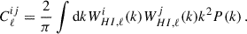
2. The Cℓ of the HI brightness temperature
In IM experiments, the brightness temperature of the HI (neutral hydrogen) line is used to study the LSS of the Universe. Such emission results from a transition between two energy levels of the hydrogen atom, corresponding to the hyperfine structure. The emission in the rest frame has a wavelength of 21 cm and the corresponding frequency of ν10 = 1420 MHz. Following Furlanetto et al. (2006), Pritchard & Loeb (2012), the observed (average) 21 cm brightness temperature at low-redshifts, z < 2, is
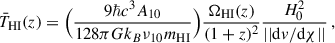 (1)
(1)
where H0 is the Hubble constant and ||dv/dχ|| is the gradient of the specific velocity field along the line of sight and ΩHI(z) is the density parameter of HI. The constants G, c, kB, and ℏ are the gravitational constant, speed of light, Boltzmann constant, and reduced Planck constant, respectively. Also, A10 represents the spontaneous emission coefficient of the 21 cm transition, and mHI is the HI atom mass. Following Battye et al. (2013), Hall et al. (2013) this expression gets simplified by referring to the cosmic background evolution, where we can express the gradient of the specific velocity only in terms of Hubble flow;
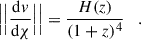 (2)
(2)
By replacing the values of the fundamental constants, we found
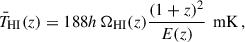 (3)
(3)
where H0 = 100 h km s−1Mpc−1 and E(z) = H(z)/H0.
Like the dark matter distribution, the brightness temperature is not homogeneously distributed, and by considering its spatial anisotropy,  , we depict the temperature field as
  , where
  is the unit vector along the line of sight (LoS). The temperature fluctuation ΔTHI results from various mechanisms during the cosmic evolution, including the foremost contribution from the HI overdensity δHI, and approximately we have
  .
.
Since 21 cm IM surveys the Universe within tomographic frequency channels (or equivalently, frequency bins), the observable in practice is a projection of the 3D temperature field along LoS, such that the integrated temperature fluctuation reads
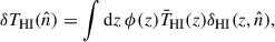 (4)
(4)
where ϕ(z) is the window function determining the bin width. Assuming a top-hat filter, we have ϕ(z) = 1/(zmax − zmin) for zmin < z < zmax and ϕ(z) = 0 outside the frequency channel (Battye et al. 2013).
Following Novaes et al. (2022), the resulting angular power spectrum  for the projected HI brightness temperature is
 (5)
(5)
where the indices i, j denote tomographic frequency channels such that, for i = j and i ≠ j, we obtain auto- and cross-APS, respectively. The WHI, ℓi term is a window function collecting all the redshift dependencies;
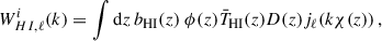 (6)
(6)
where D(z) is the growth function, bHI(z) is the HI bias as a function of the redshift, and jℓ is the spherical Bessel function. Equation (6) depends on two parameters of the HI astrophysics, bHI(z) and ΩHI(z) (through Eq. (3)). For simplicity, we assume that the frequency channels are sufficiently thin, such that both parameters can be assumed to have constant values inside each bin. We also assume them to be scale-independent.
In our work, we use the UCLCl code (McLeod et al. 2017; Loureiro et al. 2019b) a library for calculating the angular power spectrum of the cosmological fields. Such code obtains the primordial power spectra and transfer functions from the CLASS Boltzmann code (Blas et al. 2011) and applies Eq. (5) to obtain the APS. In the UCLCl, the Cℓ computation may be extended some way into the non-linear regime by introducing the scale-dependent non-linear overdensity δNL(k, χ) from the CLASS code (Blas et al. 2011; Di Dio et al. 2013), using the modified HALOFIT of Takahashi et al. (2012). See Loureiro et al. (2019b) for details.
2.1. Redshift space distortion
Galaxies have peculiar velocities relative to the overall expansion of the Universe. This creates the illusion that the local peculiar motion of galaxies moving towards us makes them appear closer (i.e., appear to be at lower redshifts), while galaxies with peculiar motion moving away from us appear to be further away (i.e., they appear to be at higher redshifts). This effect is called by redshift space distortion (RSD; Kaiser 1987), and it is also taken into account by the UCLCl code.
In this work, we follow the same formalism of Fisher et al. (1994), Padmanabhan et al. (2007). This formalism was presented for galaxy probes, and we adapted it for our IM window function. Assuming that the peculiar velocities are small compared with the thickness of the redshift slice, we write  as a function of the redshift distance
  and take the first order Taylor expansion;
 (7)
(7)
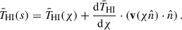
The first order term leads to a correction on the window function used in Eq. (5), which becomes WTot, ℓi = WHI, ℓi + WRSD, ℓi, with the RSD contribution given by
 (8)
(8)
![Mathematical equation: $$ \begin{aligned} &= \beta ^i \int {\mathrm{d} } \chi \, \phi ^i (\chi ) T_{\rm HI}(\chi ) \Big [ \frac{ (2\ell ^2 + 2\ell + 1) }{(2\ell +3)(2\ell -1)} j_\ell ( k\chi ) \nonumber \\&\quad {-}\ \frac{\ell (\ell -1)}{(2\ell -1)(2\ell +1)}j_{\ell -2} ( k\chi ) \nonumber \\&\quad {-}\ \frac{(\ell +1)(\ell +2)}{(2\ell +1)(2\ell +3)}j_{\ell +2} ( k\chi ) \Big ] \,, \end{aligned} $$](/articles/aa/full_html/2026/04/aa55763-25/aa55763-25-eq16.gif) (9)
(9)
where βi is the redshift distortion parameter, βi = (dlnD(z)/dlna)/bHIi. The RSD window function does not consider the Fingers of God effect, which affects small scales due to the virial motion of galaxies inside clusters (Kang et al. 2002).
2.2. Partial sky: Mixing matrix convolution
The modeling given by Eq. (5) assumes the (brightness) temperature as an isotropic random field defined in the whole sphere. However, for comparison with the data, we need to take into account that we only survey a portion of the sky. The angular mask function  can be expanded into spherical harmonics coefficients
 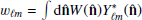 and with a power spectrum
 (10)
(10)
Following Hivon et al. (2002) and Blake et al. (2007), the effect of the angular mask function on the power spectrum is given by a convolution with a coupling kernel
 (11)
(11)
where Rℓℓ′, the mixing matrix, is given by
 (12)
(12)
The mixing matrix depends only on the mask function given by its angular power spectrum 𝒲ℓ. The 2 × 3 matrix above is the Wigner 3j function; these coefficients were calculated using the UCLWig 3j library1, which optimises the calculation of Wigner 3j symbols using the recurrence relation by Schulten & Gordon (1976).
3. BINGO simulations
The simulations used in our analysis are designed to reproduce the observational configuration of the BINGO phase 1 experiment, with parameters summarized in Table 1. Each simulated map includes the cosmological 21 cm signal, thermal instrumental noise, and the beam smoothing effect, modeled as a symmetric Gaussian with θFWHM = 40 arcmin, consistent with BINGO’s optical design. The full BINGO frequency band, spanning 980–1260 MHz, is divided into 30 tomographic bins of Δν ≈ 9.33 MHz, matching the resolution of the digital backend. Simulations are produced using the HEALPix pixelization scheme (Gorski et al. 2005) with Nside = 256, which provides an angular resolution well-suited to the telescope’s beam size.
Summary of the BINGO telescope and survey parameters (phase 1).
We generated 3000 independent realizations of the cosmological 21 cm signal. To each realization, we added one instance of thermal (white) noise and simulated astrophysical foregrounds to create a set of contaminated total sky maps. We then apply the FastICA component separation algorithm to each of these 3000 maps to perform blind foreground removal. This process yields a corresponding set of 3000 reconstructed maps, which contain the recovered 21 cm signal and instrumental noise. One randomly selected realization from this set is used as the mock data vector for cosmological inference, while the full ensemble is used to compute the covariance matrix. An example of each simulation component and their combination is shown in Figure 1.
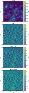 |
Fig. 1. Cartesian view of a simulated 21-cm tomography pipeline for cosmological inference. The first panel displays the pure cosmological signal generated with the FLASK code and convolved with a 40 arcmin FWHM Gaussian beam. The second panel shows a single realization of the white noise contribution. The third panel presents the combined signal and noise. The final panel shows the reconstructed signal obtained using the FastICA algorithm. |
3.1. Cosmological signal
We used the publicly available FLASK2 code (Xavier et al. 2016) to produce two-dimensional tomographic realizations (spherical shells around the observer, positioned at the center) of random astrophysical fields following a multivariate lognormal distribution, reproducing the desired cross-correlations between them. The lognormal distribution is more suitable to describe matter tracers than the Gaussian distribution, avoiding non-physical (δ < −1) densities. FLASK takes as input the auto- and cross-Cℓij (i = j and i ≠ j, respectively) previously calculated for each of the i, j redshift slices. The 21 cm Cℓij are computed with the UCLCl code using the Planck 2018 ΛCDM fiducial cosmology (Ωb = 0.0493, Ωc = 0.2645, h = 0.6736, ns = 0.9649, ln1010As = 3.044, τr = 0.0544; Planck Collaboration VI 2020) and HI parameters given by ΩHI = 3.642 × 10⁻⁴ (Padmanabhan et al. 2015) and bHI = 1. From them, we generated 3000 lognormal realizations, each of them corresponding to 30 HEALPix full sky maps of 21 cm brightness temperature fluctuations, one for each BINGO frequency (or redshift) bin. For simplicity, and following some of the previous works of the BINGO collaboration (Zhang et al. 2022; Fornazier et al. 2022), we fix the number of channels at 30 (δν = 9.33 MHz). The impact of different tomographic binning for the cosmological analyses will be evaluated in the future (see de Mericia et al. 2023, for analyses evaluating the impact of the number of frequency channels in the foreground cleaning process).
3.2. Foreground signals
Using the Planck Sky Model software (PSM; Delabrouille et al. 2013), we simulated the foreground signal contributing in each frequency bin of the BINGO band. Following Novaes et al. (2022) and de Mericia et al. (2023), we consider the contribution of seven foreground components. From our Galaxy, we account for the synchrotron and free-free emissions, which are the most important contaminants in the BINGO band, as well as the thermal dust and anomalous microwave emissions. Among the extragalactic components, we include the thermal and kinetic Sunyaev-Zel’dovich effects and the unresolved radio point sources. For a detailed description of the specific configuration adopted in the PSM code to simulate each foreground component, we refer the reader to de Mericia et al. (2023).
3.3. Instrumental effects and sky coverage
The effect of the BINGO beam is incorporated into all frequency maps by convolving them with a symmetric Gaussian profile. We adopt a fixed full-width at half maximum of θFWHM = 40 arcmin, which corresponds to the beam size at 1100 MHz. While the true beam width varies slightly with frequency, this variation is slow across the 980–1260 MHz BINGO band. Therefore, using a constant beam size across all channels is a good approximation for the purposes of our analysis. Moreover, the Gaussian profile has been shown to accurately reproduce the BINGO beam shape at the relevant frequencies, as demonstrated in Abdalla et al. (2022b). We then add to the simulations the contribution of the thermal (white) noise, taking into account the BINGO specifications, as detailed in Wuensche et al. (2022), Abdalla et al. (2022b). We note that this noise model does not include 1/f (correlated) noise, which is a common simplification for preliminary analyses. While this omission may underestimate noise correlations at large angular scales, we expect the impact to be subdominant for BINGO’s primary science goals given the scanning strategy and data processing pipelines. We assumed BINGO phase 1 operation setup, with temperature system Tsys = 70 K, operating with 28 horns and the optical arrangement as designed in Abdalla et al. (2022b), and considering 5 years of observation. To allow for a more homogeneous coverage of the BINGO region, the horns will have their positions shifted by a fraction of beam width in elevation each year. Taking these specifications into account, the thermal noise level, or the root mean square (RMS) value, by pixel, at the resolution of Nside = 256, was estimated as described in Fornazier et al. (2022). From this RMS map, we were able to generate an arbitrary number of noise realizations by multiplying it by Gaussian distributions of zero mean and unitary variance. In order to reproduce BINGO sky coverage, we also applied a cut sky mask to the simulations. Besides selecting BINGO area, this mask also cuts out the 20% more contaminated Galactic region. It is also apodized with a cosine square (C2) transition, using the NaMaster code3 (Alonso et al. 2019), to avoid boundary artifacts when calculating the APS. Details on how this mask is constructed can be found in de Mericia et al. (2023).
3.4. Foreground cleaning
Our methodology builds upon the BINGO collaboration’s framework, where previous studies have tested and compared blind component separation methods (Fornazier et al. 2022; Liccardo et al. 2022; de Mericia et al. 2023; Marins et al. 2022). Our current implementation uses the FastICA algorithm (Hyvarinen 1999), which is based on the principle of statistical independence between components. This choice is motivated by its performance in recovering the 21 cm signal with an accuracy equivalent to other blind methods, combined with a favorable computational efficiency for processing large ensembles of simulations in the current stage of our pipeline analysis (Marins et al. 2022).
We performed blind foreground removal using the Fast-ICA algorithm implemented in the scikit-learn package4. The method was applied directly to our multi-frequency simulated maps. Operating without prior templates, FastICA identifies and isolates the dominant, statistically independent foreground components. After subtracting these components from the data, the residual signal is projected back into frequency space to yield a set of foreground-cleaned maps. For our analysis of 3000 sky simulations, we configured the algorithm to estimate 4 independent components. Following the setup successfully applied in similar 21 cm IM contexts (Marins et al. 2025), we use the ‘logcosh’ nonlinearity with 20 interactions, and a convergence tolerance of 0.01.
4. APS measurements from maps
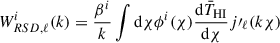
Given our simulated temperature fluctuation maps, let aℓm be the coefficients of spherical harmonic expansion. The pseudo-Cℓ estimate that takes in account beam resolution, pixelation scheme, and sky coverage corrections is defined by
 (13)
(13)
Here, bℓ is the axisymmetric beam window function, e.g., Challinor & Lewis (2011), assumed in this work as a Gaussian beam and wℓ is the pixel window function (Gorski et al. 2005; Leistedt et al. 2013). The beam window function corrects the effect of the beam resolution on the observed angular power spectrum. It was computed assuming the beam to be Gaussian with full-width half maximum of θFWHM = 40 arcmin. The pixel window function corrects a suppression of power on small scales caused by the effect of the finite size of the HEALpix pixel. For detailed discussion, we refer to the HEALpix manual5.
Although Eq. (13) provides an unbiased estimate for pure 21 cm maps, it becomes biased when applied to reconstructed maps. We employ a debiasing procedure Fornazier et al. (2022), Marins et al. (2022), de Mericia et al. (2023) to correct the estimated angular power spectrum (APS) for two effects: an additive bias from instrumental noise and a multiplicative bias arising from signal attenuation during the foreground removal process. Our debiased APS estimator is given by:
 (14)
(14)
Here,  is the biased APS estimate from a foreground-cleaned map, and
  is the ensemble average noise power spectrum estimated from random Gaussian realizations (see Sect. 3.3). The factor βℓ corrects for signal loss induced by the component separation pipeline. We estimated βℓ as:
 (15)
(15)
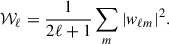
where  is the APS of the input (21 cm + white noise) simulation. The average ⟨ ⋅ ⟩ is computed, when debiasing a given target simulation, from the remaining 2999 simulations to avoid statistical coupling. A comparison of the reconstructed Cℓ, the pure 21 cm signal, and the theoretical spectrum is shown in Fig. 2.
 |
Fig. 2. Comparison of angular power spectra Sℓ for different simulated components. The solid black line shows the theoretical 21 cm spectrum from UCLCl. Colored lines represent measured spectra from simulations: pure 21 cm signal (blue), the sum of 21 cm and white noise (orange), the reconstructed spectrum after foreground removal (green, biased), and the final debiased spectrum (red) after applying the correction from Eq. (14). |
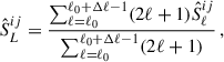
We further perform a bandwidth binning to the Sℓ estimates. This binning acts on the measurement in a way that decorrelates mixed modes. We bin the ℓ values into bins Δℓ of width 11 (so e.g., the first bin is 2 ≤ ℓ ≤ 12). For each bin, we calculated a weighted average of the  (weighted by the number of spherical harmonic coefficients),
 (16)
(16)
where ℓ0 is the first multipole of each bin, for example, 2, 13, 24, and so on. Here, L simply denotes each multipole bin.
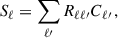
Figure 3 illustrates the relative error  , computed in relation to the UCLCl theoretical SLth at the fiducial cosmology. This plot draws attention to the behavior of the errors for a range of multipoles with respect to both the UCLCl theoretical spectrum and the standard deviation of the 3000 simulations.
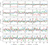 |
Fig. 3. Relative error |

While the average  values from the 3000 simulations closely track the UCLCl theoretical spectrum, it is evident that the random errors on the spectrum for individual realizations, i.e., cosmic variance, exhibit strong correlations among neighboring multipoles within the same frequency channel. Let us take, for example, the frequency channel 10. The realization depicted in blue and in green shows mostly positive errors, while the realization depicted in red show mostly negative errors within the depicted multipole range.
Figure 3 allowed us to distinguish between random and systematic errors in the power spectrum recovery. The colored lines, representing individual simulation realizations, are dominated by random errors. The correlation of these errors across neighboring multipoles is introduced by the sky mask applied to the lognormal simulations. When averaged over all realizations, however, the black line is is consistent with zero across most of the multipoles, which shows that our pipeline recovers well the theoretical spectrum. The only notable deviation is a minimal systematic bias at very low multipoles (ℓ ≲ 25), which we attribute to the foreground removal process.
5. Covariance matrix
For cosmological inference, it’s essential to quantify the uncertainties associated with the observed power spectrum. To achieve this, we calculate the covariance matrix based on a set of Nsim = 3000 BINGO simulations, as elaborated upon in section 3. Let  be the weighted estimation of the angular power spectrum of the BINGO n-th realization, the covariance matrix of the ensemble of angular power spectra is
 (17)
(17)
where  is the average pseudo-Cℓ estimate for the 3000 BINGO simulations. Figs. 4 and 5 show the Pearson correlation coefficient
 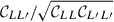 computed from the FLASK covariance matrix. The degree of correlation among different multipoles can be inferred from the diagonal properties of this matrix. The figures presented illustrate the correlation characteristics of both the pure simulated 21 cm cosmological signal and the debiased signal after accounting for systematic error sources.
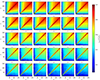 |
Fig. 4. Pearson correlation coefficient |
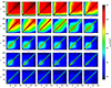 |
Fig. 5. Pearson correlation coefficient |

In both instances, the correlation decreases with the redshift, leading to matrices with more pronounced diagonal features for the latest frequency channels. This effect is due to the stronger non-Gaussian features at lower redshifts. However, a distinction arises when comparing the pure 21 cm signal’s correlation with that of the reconstructed signal incorporating systematic error sources.
The pure 21 cm signal covariance exhibits strengthening off-diagonal correlations at higher multipoles. This trend, driven by the non-Gaussian nature of the cosmological signal, is not observed in the debiased signal after white noise have been included. The reason for this divergence is the dominance of instrumental white noise at high multipoles, which follows Gaussian statistics. This substantial Gaussian noise component effectively dominates over the non-Gaussian correlations intrinsic to the 21 cm signal. Furthermore, the process of foreground reconstruction modifies the covariance structure, particularly in the earliest channels, where it introduces an increase in correlation. Thus, the final covariance of the reconstructed signal reflects these two effects combined.
6. Likelihood and sampling methods
The Bayesian framework has been widely used in cosmology to make inferences about the parameters of cosmological models in light of data from the LSS. We follow a standard Bayesian analysis framework as commonly performed in the literature, e.g., Krolewski et al. (2021), Contarini et al. (2022), Loureiro et al. (2019b), Köhlinger et al. (2017), Thomas et al. (2011), Abbott et al. (2019), Blake et al. (2007).
6.1. Priors
In this work, we take the standard approach of assuming that the priors are uniformly distributed (flat priors). Flat priors are used in order to reduce the dependence of the results on the choice of prior, allowing the data to drive the results and avoid potential biases from strong prior beliefs (Massimi 2021; Diacoumis & Wong 2019; Efstathiou 2008). The prior defined for the cosmological analysis are shown in table 2. The first block consists of six independent cosmological parameters: Ωbh2, Ωch2, 100θS, ns, ln1010As, τr, where Ωb is the baryonic matter density, Ωc is the cold dark matter density, h is the Hubble constant, As is the amplitude of the primordial power spectrum, ns is the spectral index, θs is the sound horizon at decoupling and τr is the optical depth at reionization epoch. The cosmological priors are defined to cover at least the 3σ interval of the Planck constraints from Planck Collaboration VI (2020). The second block is the HI parameters, which are two per bin: the HI bias bHIi and the HI density (ΩHIi). The HI parameters are assumed constant within each frequency channel and scale independent.
Prior ranges for cosmological analysis.
6.2. Multipole selection
While the Cℓ discussed in Section 2 incorporates dark matter non-linearities, it omits non-linear effects stemming from HI physics, such as scale-dependent bias. To address this, we opted to establish cuts in ℓmax for each tomographic frequency channel, a strategy aimed at excluding non-linear scales. We computed the linear and non-linear Cℓ at fiducial cosmology (the same used in Sect. 3.1) and performed a cut in ℓmax where the percent deviation between the linear and non-linear models were smaller than 10%. Additionally, we drop out small multipoles where foreground removal systematic errors appear. We fix ℓmin = 25 for all multipoles. The employed multipole selection, along with the bandwidth binning, yields a relatively small number of data points for the initial frequency channels. Expanding the range of ℓmax could enhance the precision of the constraints. However, given the absence of a non-linear theory for HI physics, our objective is to derive realistic constraints from the linear regime. The specific ℓmin and ℓmax values resulting from this approach for all frequency channels are presented in Table 3.
Multipole range considered for cosmological analysis.
6.3. Likelihood
The likelihood quantifies the agreement between the hypothesis and the data. Following Loureiro et al. (2019b), we assumed the likelihood to have the Gaussian form,
 (18)
(18)
where
![Mathematical equation: $$ \begin{aligned} \chi ^2 (\mathbf \Theta )&= \left[ \hat{S}_{L} - S^{th}_{L}(\mathbf \Theta )\right]^T \mathcal{C} ^{-1} \left[ \hat{S}_{L} - S^{th}_{L}(\mathbf \Theta )\right] \,. \end{aligned} $$](/articles/aa/full_html/2026/04/aa55763-25/aa55763-25-eq40.gif) (19)
(19)
The  is the pseudo-APS estimate measured from our dataset as described in Sect. 4,
  is the theoretical spectrum calculated with UCLCl code following the Sect. 2 after being convolved with the mixing matrix (Eq. (11)) and being binned with the same bandwidth of the data (Eq. (16)). Finally, 𝒞 is the covariance matrix described in Sect. 4 encapsulating the uncertainties and correlations between the data points.
The presented likelihood function (Eq. (18)) is based on the assumption that the observed data follows a Gaussian distribution. However, this approximation is imperfect due to the lognormal field’s inherent non-Gaussian characteristics. To explore the potential of non-Gaussian likelihoods, further investigation and testing could be pursued in future endeavors.
Tighter constraints on the cosmological parameters can be obtained by combining BINGO with the Planck 2018 dataset. Assuming that each probe provides independent information, the joint likelihood is
 (20)
(20)
The CMB data from Planck was added through the Planck likelihood codes Commander and Plik (Planck Collaboration V 2020). We include in our analysis the likelihoods lowlTT (temperature data over 2 ≤ ℓ ≤ 30), Planck TT,TE,EE (the combination of Planck TT, Planck TE, and Planck EE, taking into account correlations between the TT, TE, and EE spectra at ℓ > 29), lowE (the EE power spectrum over 2 ≤ ℓ ≤ 30) and the Planck CMB lensing likelihood. The multiplication of these four likelihoods is commonly referred as Planck TT,TE,EE+lowE+lensing.
6.4. Sampling
Sampling points in parameter space play a crucial role in Bayesian inference, as they allow us to estimate the posterior distribution of the parameters. Some traditional Markov chain Monte Carlo (MCMC) methods are Metropolis–Hastings (Metropolis et al. 1953; Hastings 1970), Gibbs sampling (Geman & Geman 1984), Hamiltonian sampling (Duane et al. 1987), and thermodynamic integration (Ruanaidh & Fitzgerald 2012). In our work, we use the nested sampling method (Skilling 2004, 2006). It is more efficient than traditional MCMC methods because it uses the information about the prior volume to guide the sampling instead of randomly proposing moves in the parameter space as in Metropolis–Hastings. The algorithm works by constructing a sequence of nested sets of points in parameter space, each set being a subset of the previous one, and keeping track of the points that have the highest likelihood. Multinest (Feroz & Hobson 2008; Feroz et al. 2009, 2013) is the most popular and freely accessible software package that implements the nested sampling method. In this paper, we employ Pliny (Rollins 2015), an open-source nested sampling algorithm implementation that prioritizes optimal parallel performance on both distributed and shared memory computing clusters. Pliny has been successfully applied to cosmological analysis as in McLeod et al. (2017), Loureiro et al. (2019a,b), Jeffrey & Abdalla (2019).
7. Results
In this section, we present cosmological constraints for the BINGO simulations + Planck 2018 likelihood within the framework of ΛCDM and w0waCDM cosmology. In Section 7.1, we study the consistency of parameter constraints across different realizations of the pure 21 cm cosmological signal BINGO simulation within ΛCDM cosmology. In Section 7.2 we explore the impact of white noise and residual of foreground removing on the cosmological parameter contours. In Section 7.3, we present constraints on the HI parameters, and in Section 7.4, we extend the analysis to the w0waCDM model. Finally, in Section 7.5, we discuss the goodness of the Monte Carlo fits.
7.1. Cross-checking ΛCDM constraints between different 21 cm realizations
We derived constraints on cosmological parameters by jointly analyzing simulated data from BINGO and the Planck 2018 likelihood under the assumption of a flat ΛCDM framework. Planck’s measurements provide more stringent constraints than other independent cosmological experiments, making it a robust baseline for comparison. The analysis focused on six primary cosmological parameters: the baryon density Ωbh2, cold dark matter density Ωch2, angular acoustic scale 100θs, scalar spectral index ns, amplitude of primordial fluctuations ln1010As, and optical depth to reionization τr, alongside 60 additional parameters characterizing neutral hydrogen (HI). The Hubble constant (H0) was inferred as a derived parameter from the aforementioned six. We compared results using the pseudo-Cℓ estimator across multiple realizations of the BINGO simulations, with the outcomes for three realizations illustrated in Fig. 6. See also Table 4.
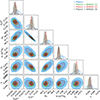 |
Fig. 6. Comparison of parameter constraints from BINGO simulations with Planck 2018 data. The blue contour shows the posterior from Planck 2018 data alone. The remaining contours combine BINGO simulations with Planck 2018 data within the ΛCDM framework. Green, red, and black dashed contours correspond to three different BINGO realizations. Dotted black lines mark the fiducial (true) parameter values. This analysis does not include systematic effects from white noise or foreground removal. Results are consistent across all BINGO realizations. |
Marginalized cosmological ΛCDM constraints and 68% credible intervals.
Initially, we examined the parameter fitting outcomes under idealized conditions, considering only the pure cosmological 21 cm signal. While this analysis excluded observational systematics such as instrumental noise and foreground contamination, it consistently accounted for the sky mask and the beam convolution. Our findings demonstrate that combining BINGO simulations with Planck 2018 data significantly improves the precision of parameter constraints compared to Planck 2018 alone. The joint analysis yields tighter posteriors that remain fully consistent with the Planck 2018 fiducial cosmology.
The joint analysis significantly tightens the constraint on the optical depth to reionization (τreio), despite the 21 cm power spectrum having no direct sensitivity to this parameter. The inclusion of BINGO simulations provides independent measurements of As and ns. By reducing uncertainties in these primordial parameters, the joint analysis indirectly diminishes the allowed range for τreio.
Notably, the probability contours exhibit slight positional shifts between different BINGO realizations. These variations arise from statistical fluctuations inherent to the simulated data and theoretical degeneracies in the parameter space. Crucially, the magnitude of these shifts aligns with the expected statistical uncertainties at the 68% and 95% confidence levels. Despite these minor displacements, the contours retain consistent shapes and sizes across all realizations, indicating robustness in the parameter estimation methodology.
7.2. Exploring ΛCDM constraints with white noise and foreground removing effects included
Initially, we examined the parameter fitting outcomes with sole consideration for the pure 21 cm cosmological signal. Although the previous section excludes observational systematics such as instrumental noise and foregrounds, the results always take into account the effects of the sky mask and beam convolution. We now extend our analysis to include the impact of white noise and foreground removal. To achieve this, both the measured Cℓ values, designated for fitting, and the associated covariance matrix were sourced from BINGO simulations that incorporated white noise, as elaborated upon in Section 3. Finally, we took into account the residual foregrounds following the methodology outlined in Section 3. The constraints are shown in Table 4 and Fig. 7.
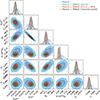 |
Fig. 7. Parameter constraints from BINGO simulations with systematic effects, combined with Planck 2018 data. The blue contour shows the posterior from Planck 2018 data alone. The green contour represents a joint constraint from Planck 2018 and a BINGO simulation containing only the cosmological 21-cm signal. The red contour uses the same 21-cm realization but with white noise added. The black dashed contour further includes the process of foreground removal. Dotted black lines mark the fiducial parameter values. |
Notably, the constrained values of the ΛCDM parameters exhibited consistent behavior across the three scenarios. The confidence levels associated with these estimates remained similar across the different cases. This indicates that systematic error sources do not increase the uncertainty surrounding our parameter estimates. The fact that the uncertainties do not increase can be explained by the high S/R within the multipole range used for the cosmological analysis and the low amplitude of the foreground removal residuals.
Our analysis underscores that incorporating BINGO data significantly refines the precision of parameter constraints in comparison to relying solely on the Planck likelihood, even when including white noise and foreground removal. For the simulation that includes white noise and foreground removal, we got Ωbh2 = 0.022309 ± 0.000072,  , H0 = 67.06 ± 0.23,
 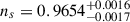 ,
,  , τr = 0.0482 ± 0.0031. This corresponds to a decrease in the confidence level with respect to the Planck-only one by 58% for Ωbh2, 61% for Ωch2 and 63% for H0.
7.3. HI parameter constraints
In this subsection, we discuss the constraints on the HI parameters for the simulations shown in the preview sections. In all of our analyzes, the parameters ΩHIbHI and bHI were treated as independent variables across all frequency channels, resulting in a total of 60 distinct HI parameters. The marginalized constraints for all 60 HI parameters with their respective 68% credible interval are displayed in Fig. 8. Aditionally, the 2D constraints on these parameters for one of the frequency channels are shown in Figs. 9. Both figures shows consistencies of the marginalized values and uncertainty levels across different scenarios, and the potential of BINGO to measure the HI history.
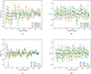 |
Fig. 8. Marginalized constraints for the 60 HI parameters and 68% credible intervals for BINGO + Planck likelihood. The dashed black lines indicate the truth (fiducial) value of the parameters. In Panels 8a and 8b, we show the constraints for the ΩHIbHI and bHI for three different realizations of the pure cosmological signal. In Panels 8c and 8d we show the constraints for three cases: simulation of the pure cosmological 21 cm signal (blue), simulation including white noise (orange), simulation including white noise and foreground removal (green). We find that we can recover the fiducial values within 1 ∼ 2σ for most of the parameters. This result shows the potential of BINGO to constrain HI history. |
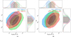 |
Fig. 9. Two-dimensional constraints of the HI parameters of the 10th frequency channel of the Planck + BINGO likelihood. Panel a shows the consistency across different realizations of of the BINGO simulations. The dotted black lines indicate the truth (fiducial) value of the parameters. Panel b compares the contours for the simulation of the pure 21 cm cosmological signal (blue), simulation including white noise (green), simulation including white noise and foreground removal (red). We find similar shapes and uncertainty levels across the comparisons. |
Figs. 8a and 8b presents the derived constraints on the HI parameters across three independent realizations of the 21 cm signal. The agreement between realizations shows that our methodology is stable against statistical variations in the input signal, with all chains converging to consistent posterior distributions.
To quantify the impact of observational effects, Figs. 8c and 8d compare constraints under three scenarios: pure cosmological signal without white noise or foreground contamination; simulation including white noise; and simulation combining effects of white noise and residual of foreground removing. The fiducial input values (indicated by dashed lines) are recovered within 1 ∼ 2σ confidence intervals for all parameters, demonstrating the statistical consistency of our pipeline. Similarly as for the cosmological parameters, the uncertainties surrounding the parameter estimates do not increase with the addition of systematic error sources. Again, it can be explained by the high S/R and low residual level within the multipole range of the fitting.
7.4. w0waCDM constraints
The constraints on the w0waCDM cosmological parameters, derived from Planck 2018 data alone and in combination with the BINGO simulation, are presented in Fig. 10. The w0waCDM model parameterizes the dark energy equation of state as w(z) = w0 + wa(1 − a) (Chevallier & Polarski 2001; Linder 2003), where w0 is its present-day value and wa quantifies redshift evolution. Our analysis reveals a marked improvement in the precision of these parameters when BINGO’s 21 cm IM data is incorporated into the Planck baseline.
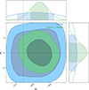 |
Fig. 10. Constraints for w0waCDM cosmology for Planck 2018 (blue) and Planck 2018 + BINGO (green). With the inclusion of the BINGO simulation data we can measure w0 and wa with a confidence level of 0.22 and 1.2. |
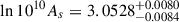
Planck 2018 alone (blue contours in Fig. 10), the posterior distributions of w0 and wa largely reflect the prior volume, consistent with the known challenge of constraining dark energy parameters using CMB data alone Planck Collaboration VI (2020). In contrast, combining Planck with BINGO’s simulated 21 cm observations (green contours) breaks this degeneracy, yielding a measurement of the dark energy equation of state consistent with the fiducial ΛCDM values (w0 = −1, wa = 0) at the 1.9σ confidence level. The joint constraints are:
 (21)
(21)
This demonstrates BINGO’s potential to probe the nature of dark energy. Although Planck yields precise measurements for most of the cosmological parameters, BINGO complements Planck by anchoring the low-redshift expansion history, where dark energy dominates.
7.5. Goodness of the fits
We calculated the overall reduced χ2 for the Monte Carlo fits presented in this paper. The overall reduced χ2 is defined as χred2 = χ2/(Nd − Np), where Nd is the number of data points and Np is the number of parameters. Given the chosen bandwidth binning and multipole selection for our analysis, the total number of data points is Nd = 206. The number of parameters, Np is 66 (6 cosmological + 60 HI parameters) for the ΛCDM simulations. When w0 and wa parameters are included, the number of parameters is 68. Fig. 11 visualizes the best-fit theoretical curve and corresponding data points.
 |
Fig. 11. Comparison of best-fit theoretical and simulated angular power spectra for BINGO frequency channels. The blue solid curve shows the best-fit theoretical angular power spectrum (SL) derived from the optimal cosmological and hydrogen intensity (HI) parameters. Orange points represent simulated BINGO data, including contributions from white noise and foreground removal. Error bars indicate the 1σ uncertainty on SL, computed as the standard deviation across 3000 mock realizations. For each frequency channel, the number of data points (Nd) and the reduced χ2 statistic (χ2/Nd) are provided to quantify the agreement between theory and simulation. |
Table 5 showcases the χred2 values for different realizations of the BINGO simulation. These values span from 1.13 to 1.32 showing they have overall good fits with χred2 values close to one.
Overall reduced χ2 for different simulations and cosmological models.
Table 5 also provides χred2 values for three different scenarios: pure 21 cm signal, 21 cm signal with added random white noise, and 21 cm signal with both random white noise and systematic effects from foreground removal. The inclusion of white noise and foreground removal systematic effects leads to a minimal increase in χred2 compared to the parameter fitting using only the pure 21 cm signal. The w0waCDM fitting also led to a minimal increase in χred2, although a decrease in the total χ2. All this cases suggest consistency in the quality of the fitting across the different scenarios of error sources and cosmological models.
8. Conclusions
In this study, we have analyzed the potential of the BINGO 21 cm IM experiment, combined with Planck 2018 CMB data, to constrain cosmological parameters. For the ΛCDM model, we jointly constrained six core parameters (Ωbh2, Ωch2, 100θs, ns, ln1010As, and τreio) alongside 60 HI parameters and extended this framework to the w0waCDM model by including dark energy parameters w0 and wa. Combining BINGO simulations with Planck data tightens cosmological parameter constraints to ∼40% of the size of those from Planck alone (a 60% reduction), with posteriors fully consistent with the fiducial Planck cosmology.
We compared cosmological constraints across different BINGO simulation realizations and found only minor variations between them. The probability contours exhibit small displacements that align within the expected 68% and 95% confidence intervals, consistent with statistical uncertainties inherent to the simulated data. These fluctuations arise from both statistical noise in the simulations and theoretical degeneracies in the parameter space, underscoring the robustness of our methodology while highlighting the stability of the results across realizations.
The inclusion of white noise and foreground removal in our analysis revealed the robustness of the BINGO–Planck joint constraints. While white noise introduces random fluctuations mimicking instrumental uncertainties, and foreground removal adresses systematic biases from imperfect separation of galactic/intergalactic signals, our parameter estimates remained stable. We found similar confidence levels across the studied scenarios: the pure cosmological 21 cm signal, the cosmological 21 cm signal with white noise added, and the reconstructed signal after full foreground removal (which includes white noise). This resilience is explained by BINGO’s high signal-to-noise ratio (S/R) within the multipole range (ℓ < 165) used for cosmological inference, where the 21 cm signal dominates over noise.
This forecast is built upon a pipeline that implements full, blind foreground removal. The constraints presented are consequently robust against this systematic. However, several simplifying assumptions remain in our simulation framework, which the reader should consider when assessing the robustness of our results. These include the use of a Gaussian beam approximation, spectrally smooth foreground components, stationary white noise, and lognormal HI maps without non-linear clustering. These necessary and standard choices for a large-scale forecasting exercise define an optimistic but well-controlled benchmark. They successfully demonstrate the fundamental statistical power of BINGO and the efficacy of our debiasing method, while clearly identifying where future work must incorporate more complex instrumental and astrophysical systematics to transition to observational analysis.
Our analysis demonstrates BINGO’s capability to reconstruct the evolution of neutral hydrogen (HI) across cosmic time through measurements of ΩHIbHI and bHI over 30 independent frequency channels. We found consistent parameter constraints across multiple realizations and observational scenarios, even in the presence of realistic noise and residual foreground contamination. Fiducial values were recovered within 1–2σ confidence intervals across frequency channels. However, we note that the quality of foreground reconstruction can affect parameter recovery for ΩHIbHI in frequency bins where foreground contamination is most significant.
Moreover, we demonstrated the potential of BINGO to measure the dark energy equation of state. The joint Planck 2018 + BINGO analysis yielded 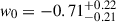 and wa = 0.0 ± 1.2, consistent with the fiducial ΛCDM values (w0 = −1, wa = 0) at the 1.9σ confidence level. While Planck provides high-precision measurements of most cosmological parameters, BINGO spans the low-redshift expansion history–the regime where dark energy dominates.
In conclusion, this study quantifies the reliability and accuracy of our cosmological parameter constraints using BINGO simulations in conjunction with Planck data. By exploring uncertainties and testing multiple simulation realizations, we demonstrate BINGO’s promising potential for constraining cosmological parameters, HI history, and the dark energy equation of state. However, our simulations simplify observational complexity: instrumental effects such as beam structure, 1/f noise, and polarization leakage require more realistic modeling in future work. This analysis represents a critical first step in validating BINGO’s capabilities. Next steps will prioritize improving simulations by addressing these systematics to strengthen BINGO’s role in probing cosmic acceleration.
Our analysis demonstrates improved cosmological constraints using BINGO simulations combined with the Planck 2018 likelihoods. However, two aspects of the fitting method could be refined in future work. First, the use of two HI-free parameters per frequency channel (totaling 60) introduces computational complexity and parameter degeneracies. Adopting a two-degree polynomial model for ΩHI and bHI across BINGO’s redshift range (Zhang et al. 2022) could reduce these to six parameters, significantly streamlining the analysis. Second, while the Gaussian approximation in our likelihood function performs adequately for the cases studied here, it may not fully capture non-Gaussian features inherent to the data. To address this, we aim to implement more robust likelihoods in future analyses.
Acknowledgments
The BINGO project is supported by FAPESQ-PB, the State of Paraiba, FINEP, and FAPESP-SP, Brazil, by means of several grants. The authors acknowledge the National Laboratory for Scientific Computing (LNCC/MCTI, Brazil) for providing HPC resources of the SDumont supercomputer, which have contributed to the research results reported within this paper. URL: http://sdumont.lncc.br. P.M.: This study was financed in part by the São Paulo Research Foundation (FAPESP) through grant 2021/08846-2 and 2023/07728-1. Also, this study was financed in part by the Coordenação de Aperfeiçoamento de Pessoal de Nível Superior – Brasil (CAPES) – Finance Code 001. F.B.A thanks the University of Science and Technology of China and the Chinese Academy of Science for grant number KY2030000215. C.P.N. thanks Serrapilheira Institute and São Paulo Research Foundation (FAPESP; grant 2019/06040-0) for financial support. E.A. is supported by a CNPq grant. E.J.M. thanks INPE for the financial support provided by the PCI fellowship. GAH acknowledges the funding from the Dean’s Doctoral Scholarship by the University of Manchester. L.O.P. acknowledges the grant 2023/07564-9, São Paulo Research Foundation (FAPESP). A.R.Q. work is supported by FAPESQ-PB. A.R.Q. acknowledges support by CNPq under process number 310533/2022-8. C.A.W. thanks CNPq for grants 407446/2021-4 and 312505/2022-1, the Brazilian Ministry of Science, Technology and Innovation (MCTI) and the Brazilian Space Agency (AEB) who supported the present work under the PO 20VB.0009.
References
- Abbott, T., Abdalla, F., Avila, S., et al. 2019, Phys. Rev. D, 99, 123505 [NASA ADS] [CrossRef] [Google Scholar]
- Abbott, T., Aguena, M., Alarcon, A., et al. 2022, Phys. Rev. D, 105, 023520 [NASA ADS] [CrossRef] [Google Scholar]
- Abdalla, E., & Marins, A. 2020, Int. J. Mod. Phys. D, 29, 2030014 [NASA ADS] [CrossRef] [Google Scholar]
- Abdalla, E., Ferreira, E. G., Landim, R. G., et al. 2022a, A&A, 664, A14 [NASA ADS] [CrossRef] [EDP Sciences] [Google Scholar]
- Abdalla, F. B., Marins, A., Motta, P., et al. 2022b, A&A, 664, A16 [NASA ADS] [CrossRef] [EDP Sciences] [Google Scholar]
- Alam, S., Ata, M., Bailey, S., et al. 2017, MNRAS, 470, 2617 [Google Scholar]
- Alonso, D., Bull, P., Ferreira, P. G., & Santos, M. G. 2015, MNRAS, 447, 400 [NASA ADS] [CrossRef] [Google Scholar]
- Alonso, D., Sanchez, J., & Slosar, A. 2019, MNRAS, 484, 4127 [Google Scholar]
- Anderson, L., Aubourg, E., Bailey, S., et al. 2012, MNRAS, 427, 3435 [Google Scholar]
- Anderson, C., Luciw, N., Li, Y.-C., et al. 2018, MNRAS, 476, 3382 [NASA ADS] [CrossRef] [Google Scholar]
- Bandura, K., Addison, G. E., Amiri, M., et al. 2014, SPIE, 9145, 914522 [Google Scholar]
- Battye, R. A., & Moss, A. 2014, Phys. Rev. Lett., 112, 051303 [Google Scholar]
- Battye, R., Browne, I., Dickinson, C., et al. 2013, MNRAS, 434, 1239 [NASA ADS] [CrossRef] [Google Scholar]
- Bernal, J. L., Bull, P., Camera, S., et al. 2025, MNRAS, 537, 3632 [Google Scholar]
- Beutler, F., Blake, C., Colless, M., et al. 2011, MNRAS, 416, 3017 [NASA ADS] [CrossRef] [Google Scholar]
- Bigot-Sazy, M. A., Ma, Y. Z., Battye, R. A., et al. 2015, ArXiv e-print [arXiv:1511.03006] [Google Scholar]
- Blake, C., Collister, A., Bridle, S., & Lahav, O. 2007, MNRAS, 374, 1527 [NASA ADS] [CrossRef] [Google Scholar]
- Blake, C., Kazin, E. A., Beutler, F., et al. 2011, MNRAS, 418, 1707 [NASA ADS] [CrossRef] [Google Scholar]
- Blas, D., Lesgourgues, J., & Tram, T. 2011, JCAP, 2011, 034 [Google Scholar]
- Bull, P., Ferreira, P. G., Patel, P., & Santos, M. G. 2015, ApJ, 803, 21 [NASA ADS] [CrossRef] [Google Scholar]
- Camacho, H., Kokron, N., Andrade-Oliveira, F., et al. 2019, MNRAS, 487, 3870 [NASA ADS] [CrossRef] [Google Scholar]
- Challinor, A., & Lewis, A. 2011, Phys. Rev. D, 84, 043516 [NASA ADS] [CrossRef] [Google Scholar]
- Chang, T.-C., Pen, U.-L., Bandura, K., & Peterson, J. B. 2010, Nature, 466, 463 [Google Scholar]
- Chen, X. 2012, Int. J. Mod. Phys. Conf. Ser., 12, 256 [NASA ADS] [CrossRef] [Google Scholar]
- Chevallier, M., & Polarski, D. 2001, Int. J. Mod. Phys. D, 10, 213 [Google Scholar]
- Chimento, L. P., Jakubi, A. S., Pavon, D., & Zimdahl, W. 2003, Phys. Rev. D, 67, 083513 [NASA ADS] [CrossRef] [Google Scholar]
- Colless, M., Dalton, G., Maddox, S., et al. 2001, MNRAS, 328, 1039 [Google Scholar]
- Contarini, S., Verza, G., Pisani, A., et al. 2022, A&A, 667, A162 [NASA ADS] [CrossRef] [EDP Sciences] [Google Scholar]
- Costa, A. A., Landim, R. C. G., Wang, B., & Abdalla, E. 2018, Eur. Phys. J. C, 78, 746 [Google Scholar]
- Costa, A. A., Landim, R. G., Novaes, C. P., et al. 2022, A&A, 664, A20 [NASA ADS] [CrossRef] [EDP Sciences] [Google Scholar]
- Cunnington, S., Wolz, L., Pourtsidou, A., & Bacon, D. 2019, MNRAS, 488, 5452 [Google Scholar]
- De Haan, T., Benson, B., Bleem, L., et al. 2016, ApJ, 832, 95 [NASA ADS] [CrossRef] [Google Scholar]
- de Mericia, E. J., Santos, L. C., Wuensche, C. A., et al. 2023, A&A, 671, A58 [NASA ADS] [CrossRef] [EDP Sciences] [Google Scholar]
- Delabrouille, J., Betoule, M., Melin, J.-B., et al. 2013, A&A, 553, A96 [NASA ADS] [CrossRef] [EDP Sciences] [Google Scholar]
- DESI Collaboration (Aghamousa, A., et al.) 2016, ArXiv e-print [arXiv:1611.00036] [Google Scholar]
- DESI Collaboration (Karim, M. A., et al.) 2025, Phys. Rev. D, 112, 083515 [Google Scholar]
- DESI Collaboration (Levi, M., et al.) 2013, ArXiv e-print [arXiv:1308.0847] [Google Scholar]
- Di Dio, E., Montanari, F., Lesgourgues, J., & Durrer, R. 2013, JCAP, 2013, 044 [CrossRef] [Google Scholar]
- Diacoumis, J. A., & Wong, Y. Y. 2019, JCAP, 2019, 025 [Google Scholar]
- dos Santos, M. V., Landim, R. G., Hoerning, G. A., et al. 2024, A&A, 681, A120 [NASA ADS] [CrossRef] [EDP Sciences] [Google Scholar]
- Duane, S., Kennedy, A. D., Pendleton, B. J., & Roweth, D. 1987, Phys. Lett. B, 195, 216 [CrossRef] [Google Scholar]
- Efstathiou, G. 2008, MNRAS, 388, 1314 [Google Scholar]
- Feroz, F., & Hobson, M. P. 2008, MNRAS, 384, 449 [NASA ADS] [CrossRef] [Google Scholar]
- Feroz, F., Hobson, M., & Bridges, M. 2009, MNRAS, 398, 1601 [NASA ADS] [CrossRef] [Google Scholar]
- Feroz, F., Hobson, M. P., Cameron, E., & Pettitt, A. N. 2013, ArXiv e-print [arXiv:1306.2144] [Google Scholar]
- Fisher, K. B., Scharf, C. A., & Lahav, O. 1994, MNRAS, 266, 219 [NASA ADS] [CrossRef] [Google Scholar]
- Fornazier, K. S., Abdalla, F. B., Remazeilles, M., et al. 2022, A&A, 664, A18 [NASA ADS] [CrossRef] [EDP Sciences] [Google Scholar]
- Furlanetto, S. R., Oh, S. P., & Briggs, F. H. 2006, Phys. Rep., 433, 181 [Google Scholar]
- Geman, S., & Geman, D. 1984, IEEE Trans. Pattern Anal. Mach. Intell., 721 [Google Scholar]
- Gong, Y., Liu, X., Cao, Y., et al. 2019, ApJ, 883, 203 [NASA ADS] [CrossRef] [Google Scholar]
- Gorski, K. M., Hivon, E., Banday, A. J., et al. 2005, ApJ, 622, 759 [Google Scholar]
- Green, J., Schechter, P., Baltay, C., et al. 2012, ArXiv e-print [arXiv:1208.4012] [Google Scholar]
- Hall, A., Bonvin, C., & Challinor, A. 2013, Phys. Rev. D, 87, 064026 [NASA ADS] [CrossRef] [Google Scholar]
- Hamann, J., & Hasenkamp, J. 2013, JCAP, 2013, 044 [CrossRef] [Google Scholar]
- Hastings, W. K. 1970, Biometrika, 57, 97 [Google Scholar]
- Hildebrandt, H., Viola, M., Heymans, C., et al. 2017, MNRAS, 465, 1454 [Google Scholar]
- Hivon, E., Górski, K. M., Netterfield, C. B., et al. 2002, ApJ, 567, 2 [NASA ADS] [CrossRef] [Google Scholar]
- Hoerning, G. A., Landim, R. G., Ponte, L. O., et al. 2025, Phys. Rev. D, 112, 023523 [Google Scholar]
- Hyvarinen, A. 1999, IEEE Trans. Neural Netw., 10, 626 [Google Scholar]
- Hyvärinen, A., & Oja, E. 2000, Neural Netw., 13, 411 [CrossRef] [Google Scholar]
- Ivezic, Z., Tyson, J., Axelrod, T., et al. 2009, Am. Astron. Soc. Meet. Abstr., 213, 460 [Google Scholar]
- Ivezić, Ž., Kahn, S. M., Tyson, J. A., et al. 2019, ApJ, 873, 111 [Google Scholar]
- Jeffrey, N., & Abdalla, F. B. 2019, MNRAS, 490, 5749 [Google Scholar]
- Jones, D. H., Read, M. A., Saunders, W., et al. 2009, MNRAS, 399, 683 [Google Scholar]
- Kaiser, N. 1987, MNRAS, 227, 1 [Google Scholar]
- Kang, X., Jing, Y., Mo, H., & Börner, G. 2002, MNRAS, 336, 892 [Google Scholar]
- Kazin, E. A., Koda, J., Blake, C., et al. 2014, MNRAS, 441, 3524 [NASA ADS] [CrossRef] [Google Scholar]
- Köhlinger, F., Viola, M., Joachimi, B., et al. 2017, MNRAS, 471, 4412 [Google Scholar]
- Kovetz, E. D., Viero, M. P., Lidz, A., et al. 2017, ArXiv e-print [arXiv:1709.09066] [Google Scholar]
- Krolewski, A., Ferraro, S., & White, M. 2021, JCAP, 2021, 028 [CrossRef] [Google Scholar]
- Laureijs, R., Amiaux, J., Arduini, S., et al. 2011, ArXiv e-print [arXiv:1110.3193] [Google Scholar]
- Leistedt, B., Peiris, H. V., Mortlock, D. J., Benoit-Lévy, A., & Pontzen, A. 2013, MNRAS, 435, 1857 [Google Scholar]
- Liccardo, V., de Mericia, E. J., Wuensche, C. A., et al. 2022, A&A, 664, A17 [NASA ADS] [CrossRef] [EDP Sciences] [Google Scholar]
- Linder, E. V. 2003, Phys. Rev. Lett., 90, 091301 [Google Scholar]
- Loureiro, A., Cuceu, A., Abdalla, F. B., et al. 2019a, Phys. Rev. Lett., 123, 081301 [NASA ADS] [CrossRef] [Google Scholar]
- Loureiro, A., Moraes, B., Abdalla, F. B., et al. 2019b, MNRAS, 485, 326 [NASA ADS] [CrossRef] [Google Scholar]
- Marins, A., Abdalla, F. B., Fornazier, K. S., et al. 2022, ArXiv e-print [arXiv:2209.11701 [Google Scholar]
- Marins, A., Feng, C., & Abdalla, F. B. 2025, ApJS, 278, 32 [Google Scholar]
- Massimi, M. 2021, Eur. J. Philos. Sci., 11, 29 [Google Scholar]
- Masui, K., Switzer, E., Banavar, N., et al. 2013, ApJ, 763, L20 [Google Scholar]
- McLeod, M., Balan, S. T., & Abdalla, F. B. 2017, MNRAS, 466, 3558 [NASA ADS] [CrossRef] [Google Scholar]
- Metropolis, N., Rosenbluth, A. W., Rosenbluth, M. N., Teller, A. H., & Teller, E. 1953, J. Chem. Phys., 21, 1087 [Google Scholar]
- Miao, H., Gong, Y., Chen, X., et al. 2023, MNRAS, 519, 1132 [Google Scholar]
- Nan, R., Li, D., Jin, C., et al. 2011, Int. J. Mod. Phys. D, 20, 989 [Google Scholar]
- Novaes, C. P., Zhang, J., de Mericia, E. J., et al. 2022, A&A, 666, A83 [NASA ADS] [CrossRef] [EDP Sciences] [Google Scholar]
- Novaes, C. P., de Mericia, E. J., Abdalla, F. B., et al. 2024, MNRAS, 528, 2078 [Google Scholar]
- Olivari, L., Remazeilles, M., & Dickinson, C. 2016, MNRAS, 456, 2749 [NASA ADS] [CrossRef] [Google Scholar]
- Olivari, L., Remazeilles, M., & Dickinson, C. 2018, Peering towards Cosmic Dawn, 333, 288 [Google Scholar]
- Padmanabhan, N., Schlegel, D. J., Seljak, U., et al. 2007, MNRAS, 378, 852 [NASA ADS] [CrossRef] [Google Scholar]
- Padmanabhan, H., Choudhury, T. R., & Refregier, A. 2015, MNRAS, 447, 3745 [Google Scholar]
- Petri, A., Liu, J., Haiman, Z., et al. 2015, Phys. Rev. D, 91, 103511 [Google Scholar]
- Planck Collaboration I. 2020, A&A, 641, A1 [NASA ADS] [CrossRef] [EDP Sciences] [Google Scholar]
- Planck Collaboration V. 2020, A&A, 641, A5 [NASA ADS] [CrossRef] [EDP Sciences] [Google Scholar]
- Planck Collaboration VI. 2020, A&A, 641, A6 [NASA ADS] [CrossRef] [EDP Sciences] [Google Scholar]
- Planck Collaboration XIII. 2016, A&A, 594, A13 [NASA ADS] [CrossRef] [EDP Sciences] [Google Scholar]
- Planck Collaboration Int. XLVIII. 2016, A&A, 596, A109 [NASA ADS] [CrossRef] [EDP Sciences] [Google Scholar]
- Pritchard, J. R., & Loeb, A. 2012, Rep. Prog. Phys., 75, 086901 [NASA ADS] [CrossRef] [Google Scholar]
- Remazeilles, M., Delabrouille, J., & Cardoso, J.-F. 2011, MNRAS, 418, 467 [Google Scholar]
- Riess, A. G., Macri, L., Casertano, S., et al. 2011, ApJ, 730, 119 [Google Scholar]
- Riess, A. G., Macri, L. M., Hoffmann, S. L., et al. 2016, ApJ, 826, 56 [Google Scholar]
- Rollins, R. P. 2015, Ph.D. Thesis, University of London [Google Scholar]
- Ross, N. P., Myers, A. D., Sheldon, E. S., et al. 2012, ApJS, 199, 3 [NASA ADS] [CrossRef] [Google Scholar]
- Ruanaidh, J. J. O., & Fitzgerald, W. J. 2012, Numerical Bayesian methods applied to signal processing (Springer Science& Business Media) [Google Scholar]
- Santos, M. G., Bull, P., Alonso, D., et al. 2015, ArXiv e-print [arXiv:1501.03989] [Google Scholar]
- Schulten, K., & Gordon, R. 1976, Comput. Phys. Commun., 11, 269 [NASA ADS] [CrossRef] [Google Scholar]
- Scolnic, D. M., Jones, D., Rest, A., et al. 2018, ApJ, 859, 101 [NASA ADS] [CrossRef] [Google Scholar]
- Skilling, J. 2004, AIP Conf. Proc., 735, 395 [Google Scholar]
- Skilling, J. 2006, Bayesian Anal., 1, 833 [Google Scholar]
- Takahashi, R., Sato, M., Nishimichi, T., Taruya, A., & Oguri, M. 2012, ApJ, 761, 152 [Google Scholar]
- The LSST Dark Energy Science Collaboration (Mandelbaum, R., et al.) 2018, ArXiv e-print [arXiv:1809.01669] [Google Scholar]
- Thomas, S. A., Abdalla, F. B., & Lahav, O. 2011, MNRAS, 412, 1669 [NASA ADS] [CrossRef] [Google Scholar]
- Troxel, M. A., MacCrann, N., Zuntz, J., et al. 2018, Phys. Rev. D, 98, 043528 [Google Scholar]
- Wang, B., Gong, Y.-G., & Abdalla, E. 2005, Phys. Lett. B, 624, 141 [Google Scholar]
- Wang, B., Abdalla, E., Atrio-Barandela, F., & Pavon, D. 2016, Rep. Prog. Phys., 79, 096901 [NASA ADS] [CrossRef] [Google Scholar]
- Wang, B., Abdalla, E., Atrio-Barandela, F., & Pavón, D. 2024, Rep. Prog. Phys., 87, 036901 [NASA ADS] [CrossRef] [Google Scholar]
- Weinberg, S. 1989, Rev. Mod. Phys., 61, 1 [NASA ADS] [CrossRef] [Google Scholar]
- Wolz, L., Abdalla, F., Blake, C., et al. 2014, MNRAS, 441, 3271 [NASA ADS] [CrossRef] [Google Scholar]
- Wuensche, C. A., Villela, T., Abdalla, E., et al. 2022, A&A, 664, A15 [NASA ADS] [CrossRef] [EDP Sciences] [Google Scholar]
- Xavier, H. S., Abdalla, F. B., & Joachimi, B. 2016, MNRAS, 459, 3693 [NASA ADS] [CrossRef] [Google Scholar]
- Xiao, L., Costa, A. A., & Wang, B. 2022, MNRAS, 510, 1495 [Google Scholar]
- York, D. G., Adelman, J., Anderson, J. E., Jr, et al. 2000, AJ, 120, 1579 [Google Scholar]
- Zhang, J., Motta, P., Novaes, C. P., et al. 2022, A&A, 664, A19 [NASA ADS] [CrossRef] [EDP Sciences] [Google Scholar]
All Tables
All Figures
|
Fig. 1. Cartesian view of a simulated 21-cm tomography pipeline for cosmological inference. The first panel displays the pure cosmological signal generated with the FLASK code and convolved with a 40 arcmin FWHM Gaussian beam. The second panel shows a single realization of the white noise contribution. The third panel presents the combined signal and noise. The final panel shows the reconstructed signal obtained using the FastICA algorithm. |
| In the text | |
|
Fig. 2. Comparison of angular power spectra Sℓ for different simulated components. The solid black line shows the theoretical 21 cm spectrum from UCLCl. Colored lines represent measured spectra from simulations: pure 21 cm signal (blue), the sum of 21 cm and white noise (orange), the reconstructed spectrum after foreground removal (green, biased), and the final debiased spectrum (red) after applying the correction from Eq. (14). |
| In the text | |
|
Fig. 3. Relative error |
| In the text | |
|
Fig. 4. Pearson correlation coefficient |
| In the text | |
|
Fig. 5. Pearson correlation coefficient |
| In the text | |
|
Fig. 6. Comparison of parameter constraints from BINGO simulations with Planck 2018 data. The blue contour shows the posterior from Planck 2018 data alone. The remaining contours combine BINGO simulations with Planck 2018 data within the ΛCDM framework. Green, red, and black dashed contours correspond to three different BINGO realizations. Dotted black lines mark the fiducial (true) parameter values. This analysis does not include systematic effects from white noise or foreground removal. Results are consistent across all BINGO realizations. |
| In the text | |
|
Fig. 7. Parameter constraints from BINGO simulations with systematic effects, combined with Planck 2018 data. The blue contour shows the posterior from Planck 2018 data alone. The green contour represents a joint constraint from Planck 2018 and a BINGO simulation containing only the cosmological 21-cm signal. The red contour uses the same 21-cm realization but with white noise added. The black dashed contour further includes the process of foreground removal. Dotted black lines mark the fiducial parameter values. |
| In the text | |
|
Fig. 8. Marginalized constraints for the 60 HI parameters and 68% credible intervals for BINGO + Planck likelihood. The dashed black lines indicate the truth (fiducial) value of the parameters. In Panels 8a and 8b, we show the constraints for the ΩHIbHI and bHI for three different realizations of the pure cosmological signal. In Panels 8c and 8d we show the constraints for three cases: simulation of the pure cosmological 21 cm signal (blue), simulation including white noise (orange), simulation including white noise and foreground removal (green). We find that we can recover the fiducial values within 1 ∼ 2σ for most of the parameters. This result shows the potential of BINGO to constrain HI history. |
| In the text | |
|
Fig. 9. Two-dimensional constraints of the HI parameters of the 10th frequency channel of the Planck + BINGO likelihood. Panel a shows the consistency across different realizations of of the BINGO simulations. The dotted black lines indicate the truth (fiducial) value of the parameters. Panel b compares the contours for the simulation of the pure 21 cm cosmological signal (blue), simulation including white noise (green), simulation including white noise and foreground removal (red). We find similar shapes and uncertainty levels across the comparisons. |
| In the text | |
|
Fig. 10. Constraints for w0waCDM cosmology for Planck 2018 (blue) and Planck 2018 + BINGO (green). With the inclusion of the BINGO simulation data we can measure w0 and wa with a confidence level of 0.22 and 1.2. |
| In the text | |
|
Fig. 11. Comparison of best-fit theoretical and simulated angular power spectra for BINGO frequency channels. The blue solid curve shows the best-fit theoretical angular power spectrum (SL) derived from the optimal cosmological and hydrogen intensity (HI) parameters. Orange points represent simulated BINGO data, including contributions from white noise and foreground removal. Error bars indicate the 1σ uncertainty on SL, computed as the standard deviation across 3000 mock realizations. For each frequency channel, the number of data points (Nd) and the reduced χ2 statistic (χ2/Nd) are provided to quantify the agreement between theory and simulation. |
| In the text | |
Current usage metrics show cumulative count of Article Views (full-text article views including HTML views, PDF and ePub downloads, according to the available data) and Abstracts Views on Vision4Press platform.
Data correspond to usage on the plateform after 2015. The current usage metrics is available 48-96 hours after online publication and is updated daily on week days.
Initial download of the metrics may take a while.