| Issue |
A&A
Volume 708, April 2026
|
|
|---|---|---|
| Article Number | A59 | |
| Number of page(s) | 12 | |
| Section | Planets, planetary systems, and small bodies | |
| DOI | https://doi.org/10.1051/0004-6361/202556139 | |
| Published online | 30 March 2026 | |
Exocomets of β Pictoris
II. Two dynamical families of exocomets simulated with REBOUND
Lund Observatory, Division of Astrophysics, Department of Physics, Lund University,
Box 118,
221 00
Lund,
Sweden
★ Corresponding author: This email address is being protected from spambots. You need JavaScript enabled to view it.
Received:
27
June
2025
Accepted:
18
February
2026
Abstract
Aims. We investigate the dynamical evolution of particles in the β Pic system to determine likely formation pathways to the exocomet populations observed in the present day. We aim to relate these results to similar studies recently carried out since the discovery of the inner planet β Pic c.
Methods. We simulated the β Pic system using the non-symplectic adaptive N-body integrator IAS15 in REBOUND. We seeded the system with over 100 000 mass-less test particles that were evolved for 25 Myr. We adopted initial conditions and a particle distribution that closely match those used in similar simulations in recent works. Using IAS15, REBOUND resolves close encounters between test particles and the two gas giants in the system, which is crucial for understanding aspects of the dynamical evolution.
Results. Planet-disc interactions rapidly clear most of the system within 35 AU, apart from a region within the orbit of β Pic c and a region between 20 and 25 AU. After 10 Myr, exocomets can be sourced continuously from these regions, as well as from the inner edge of the region beyond ∼35 AU, where particles are stable on longer timescales. From the region interior to β Pic c, the exocomets are formed by excitation via mean-motion resonance with β Pic c, obtaining a narrow distribution of radial velocities, consistent with spectroscopic observations. Particles initialised in the outer system might enter onto star-grazing orbits, due to disruption by the two gas giants, causing a wider radial velocity distribution, and we propose that this population corresponds to a second dynamical family previously observed via spectroscopy. These particles typically undergo chaotic dynamical evolution for 102−103 years after passing the water sublimation limit at ∼8 AU, before reaching the sublimation distance of calcium near 0.4 AU, implying that the two families of exocomets could have different volatile contents. This dynamical simulation depends on the assumed initial conditions, including the system parameters and the morphology of the initial disc, precluding accurate predictions of the absolute rates at which particles are generated from within and from the exterior of the orbits of the two gas giants. However, we predict that it is a general property of the system that a fraction of particles that originates from outside of the orbit of β Pic b can be scattered onto star-grazing orbits.
Key words: planets and satellites: dynamical evolution and stability / planets and satellites: individual: beta Pictoris
© The Authors 2026
 Open Access article, published by EDP Sciences, under the terms of the Creative Commons Attribution License (https://creativecommons.org/licenses/by/4.0), which permits unrestricted use, distribution, and reproduction in any medium, provided the original work is properly cited.
This article is published in open access under the Subscribe to Open model. This email address is being protected from spambots. You need JavaScript enabled to view it. to support open access publication.
1 Introduction
Beta Pictoris (β Pic) is a young nearby stellar system located at a distance of 19.28 ± 0.19 pc (Crifo et al. 1997) and estimated to be 23 million years old (Mamajek & Bell 2014). The system consists of an A-type star surrounded by a large circumstellar debris disc that is seen edge-on from Earth (Smith & Terrile 1984), which has been a subject of interest since its discovery in the early 1980s. It was discovered using the Infrared Astronomy Satellite (IRAS) through its infrared excess (Aumann 1985) and later directly imaged (Smith & Terrile 1984). The disc was observed to be warped (Burrows et al. 1995) and early on this was recognised as evidence for the gravitational influence of one or multiple unseen exoplanets (e.g. Mouillet et al. 1997). Over a decade later, the ~12 MJ planet β Pic b was finally discovered via direct imaging in a 20-year orbit at a distance of 9.91 AU (Lagrange et al. 2010; Lacour et al. 2021). A long-term radial velocity follow-up later revealed the presence of β Pic c (Lagrange et al. 2019), orbiting interior to planet b with a semi-major axis of 2.70 AU and an orbital period of 3.4 years, with a similarly high mass as the outer planet. This planet was rapidly followed up and confirmed by high-contrast interferometry observations (Nowak et al. 2020).
The relative proximity and youth of the system make it a valuable laboratory for studies of planet formation environments. Notably, the system is being observed intensively with the newly commissioned James Webb Space Telescope (JWST), enabling unprecedented new observations of β Pic b as well as the disc (e.g. Kammerer et al. 2024; Chen et al. 2024; Worthen et al. 2024).
Non-photospheric absorption features have been observed in the spectrum of β Pic since over 35 years (Ferlet et al. 1987). These observations have mainly been made in the cores of the deep stellar Ca II K and H lines at 393.366 and 396.847 nm, respectively (Edlén & Risberg 1956), where there is a stable narrow component at a radial velocity close to the systemic velocity attributed to circumstellar gas sourced from the debris disc (Slettebak & Carpenter 1983; Hobbs et al. 1985), as well as additional absorbing components that are highly variable and mostly occur at radial velocities redshifted by tens of km/s from the narrow component (Ferlet et al. 1987). On account of their redshifts, the bodies sourcing the variable absorption lines are on trajectories towards the star and these observations were quickly interpreted as absorption from sublimated material released from star-grazing planetesimals transiting in front of the star; these are known as falling evaporating bodies (FEB) or exocomets (e.g. Ferlet et al. 1987; Lagrange-Henri et al. 1988; Beust et al. 1990). Since the first spectroscopic observations of the β Pic system, many thousands of high-resolution spectra have been obtained, forming a large sample of observations of transiting exocomets from which their statistical properties can be derived (e.g. Kiefer et al. 2014). Transits of exocomets have also been observed in broad-band light-curves obtained with the Transiting Exoplanet Survey Satellite (TESS; Zieba et al. 2019).
The large radial velocities and violent sublimation observed spectroscopically imply a dynamically excited inner system. For this reason, the existence of exocomets was already used as evidence for the presence of gas giants in the inner system before these were directly detected (Beust et al. 1990). It is now well known that the orbits of planetesimals in the disc may evolve to eccentric star-grazing orbits due to gravitational interactions with the gas giants (e.g. Beust et al. 2024).
Since the first discovery of exocomets, studies based on dynamical simulations have identified resonant perturbations with an unseen planet as a likely source of exocomet progenitors (Beust & Morbidelli 1996). In this scenario, exocomet progenitors are sourced from inner mean-motion resonances (MMR) with the planet (e.g. 3:1 or 4:1) that is itself on an eccentric orbit, gradually increasing their eccentricity until they become star-grazing (Yoshikawa 1989). This model has been invoked to explain a crucial observational property of the infalling exocomet population: the majority of exocomet events are red-shifted, implying a preferred directionality in their infalling trajectories. Resonant orbital evolution with an eccentric planet would naturally result in a directional eccentricity enhancement, determined by the orientation of the orbit of the eccentric planet; thus, the mean-motion resonant model has been the leading hypothesis to explain the observed exocomet phenomenon. It was suspected that the orbital characteristics of β Pic b could fit this model (Chauvin et al. 2012; Kiefer et al. 2014), but the discovery of β Pic c as a massive gas giant interior to β Pic b (Lagrange et al. 2019) has made the system more complex than anticipated. A new numerical study was recently carried out by Beust et al. (2024), finding that the MMR model can still explain the exocomet phenomenon, albeit with progenitor particles sourced from mean-motion resonant regions within a pseudo-stable disc interior to the orbit of β Pic c, with an extent of up to 1.5 AU from the star.
Most previous numerical simulations of the orbital evolution of planetesimals in the β Pic system have been carried out with symplectic integrators (most recently by Beust et al. 2024). Symplectic integrators offer the advantages of accurate long timescale stability and high computational efficiency needed to evolve large numbers of particles, but might struggle to resolve close encounters between test particles and the planets. Potentially, the first use of a non-symplectic N-body simulation to model the dynamics of exocomets in β Pic was recently published by Rodet & Lai (2024). These authors found that the secular evolution of planetesimals in the outer regions of β Pic could result in the efficient generation of exocomets after 10 million years (half the age of the system). This simulation was carried out with a much smaller number of particles than in the study by Beust et al. (2024) and it did not include predictions for the distribution of radial velocities of infalling comets, precluding any direct comparisons with the MMR model. Conversely, the study by Beust et al. (2024) focuses exclusively on the exocomets that are sourced by the MMR process from the region interior to the orbit of β Pic c and does not address the possibility that exocomets could be generated from the regions exterior to β Pic b.
In this paper, we carry out a focussed study of the dynamics of exocomets in β Pic with REBOUND (Rein & Liu 2012), combining the accuracy of a non-symplectic integrator to resolve close encounters at a scale similar to that achieved by Beust et al. (2024), using 133 500 mass-less test particles initialised between 0.5 and 45 AU. Our primary aims are to predict the orbital dynamics of exocomets that exist at the age of the system at around 25 million years of dynamical evolution, the nature and properties of transit events by the population of comets that is observed spectroscopically (e.g. Kiefer et al. 2014), and to establish a comparison with the dominant MMR theory, which was recently modified to predict exocomet formation from a debris disc close to the star, interior to 1.5 AU (Beust et al. 2024). As our principal aim is to carry out a comparison with the results from Beust et al. (2024), we tend to follow their choices of system parameters and initial conditions in setting up our simulation. These choices include the definition of an initial disc of test particles that is uniformly distributed in orbital distance, ranging from the inner system starting at 0.5 AU out to an outer distance of 45 AU, with randomly drawn orbital parameters that place the particles on orbits that are close to circular (see Sect. 2). We also adopted one of their solutions for the parameters of the system, originally published by Lacour et al. (2021, as given in Table 1) and also noting that Beust et al. (2024) established that their results are largely independent of this choice of solution. We also note that the choices of initial conditions by Beust et al. (2024) largely match those of Rodet & Lai (2024), including the choice of solution for the system parameters, meaning that this work enables a direct comparison with both of these previous studies. Finally, we acknowledge that this configuration of the planetesimal disc of β Pic does not correspond to the observed structure of the present-day β Pic disc, in particular, the existence of a secondary component in the outer region that is inclined with respect to the orbital plane of the planets by approximately 5° (Golimowski et al. 2006). Therefore, our simulation and the simulations that we used for our comparison (Beust et al. 2024; Rodet & Lai 2024) do not confirm whether particles in this inclined disc might also evolve to match the observed statistics (Kiefer et al. 2014). In this paper, we proceed to discuss our methodology in more detail in Sect. 2 and present the results of the simulation in Sect. 3.
2 Methods
N -body simulations of the system were performed using REBOUND, with the non-symplectic integrator IAS15. This integrator is well suited for the simulation of exocomets as it can handle close encounters and highly eccentric orbits through implementation of an adaptive step-size. Symplectic integrators are popular because of their speed compared to non-symplectic N -body integrators, along with their ability to not accumulate energy errors over long timescales (Chambers 1999). However, IAS15 has been found to preserve the symplecticity of Hamiltonian systems even better than commonly used symplectic integrators, while still being able to simulate non-Hamiltonian systems (Rein & Spiegel 2015). The behaviour seen for the energy error of IAS15 resembles a random walk that follows Brouwer’s law and this property is deemed as optimal by Rein & Spiegel (2015), who successfully used it to simulate cometary close encounters and planet-forming debris discs.
2.1 Simulation set-up
With the aim to relate to recent findings of Rodet & Lai (2024) and Beust et al. (2024), we set up a simulation of the β Pic system in REBOUND, together with a disc of mass-less test particles that represent planetesimals. The simulation uses the set of system parameters of the planets and the host star also used by Beust et al. (2024), originally measured by Lacour et al. (2021), given in Table 1. In addition to the parameters presented in Table 1, the stellar radius and planetary radii we adopted are Rstar = 1.8 R⊙ (Di Folco et al. 2004) and Rb = 1.4 RJup (GRAVITY Collaboration 2020; Worthen et al. 2024; Ravet et al. 2025). An equal radius was used for planet c, such that Rc = Rb = 1.4 RJup.
We populated the system with a disc of test particles, with orbital semi-major axes a ranging from an inner boundary at 0.5 AU to an outer boundary of 45 AU, with a uniform density of 3000 particles per AU, leading to a total of 133 500 massless test particles. The particles were initiated with small initial eccentricities, e, uniformly distributed between 0 and 0.05, and inclinations, i, uniformly distributed between 0 and 2°, respectively. The initial arguments of periastron, ω, longitudes of ascending node, Ω, and mean longitudes, l, of the test particles were drawn randomly between 0 and 360°. This follows the setup of the simulation of Beust et al. (2024) and (apart from the range in semi-major axes) it also follows the approach in Rodet & Lai (2024). These initial conditions are summarised in Table 2.
The system was simulated for 25 million years, roughly corresponding to its current age (Mamajek & Bell 2014). Particles with orbits in the vicinity of β Pic c have relatively short orbital periods and are prone to undergo many close encounters. To resolve close encounters properly, we chose to evolve particles with different maximal time steps, depending on their position in the system: particles with a periastron distance greater than 3 AU were simulated using a maximal step of 5 years−1, whereas particles with a periastron distance of less than 3 AU (either because their orbital parameters evolved during the simulation or because they were initialised on such orbits) were simulated using a maximal time step of 20 year−1. If the periastron distance of a test particle shrunk to within this 3 AU boundary, the simulation was halted and the particle was reinitialised with its last orbital parameters and continued with the finer time step for the remaining duration of the simulation, regardless of whether it would move permanently back onto wide orbits beyond β Pic b (the switch from low to high-resolution is non-reversible). The 3 AU criterion was not activated for particles for which the periastron distance shrinks only briefly during a close encounter with β Pic b, by applying an additional requirement that the position of the particle is less than 5 AU when the difference between the periastron distance and 3 AU limit is evaluated. A test of the sensitivity of the results to the time-step resolution used can be found in Appendix A.
An example showing the resulting orbit of a particle simulated with both the low- and high-resolution time steps can be found in Fig. 1. The particle is initiated in the outer system at a semi-major axis of a = 25.73 AU and, therefore, it is initially simulated with the low-resolution time step. After reaching the periastron limit, the resolution of this particle is increased in order to resolve the close encounters that are more likely to happen in the vicinity of β Pic c. If a particle was initiated within the 3 AU boundary at the start of the simulation, the particle would be simulated with the high-resolution time step for its entire lifetime.
Test particles were assumed to be mass-less, allowing each particle to be simulated on its own as well as together with other test particles1. The simulation was divided into smaller instances, containing 25 test particles each, that were then ran in parallel on different CPU cores, greatly increasing the timeefficiency of the simulation. Due to the adaptive step-size used by IAS15, particles that get close to a massive body will decrease the step-size, slowing the whole simulation down. Therefore, to optimise the total integration time further, particles were grouped based on their initial position, with all particles starting within 1 AU being run together, as these are expected to experience similar dynamical evolution pathways.
A significant number of particles may be perpetually captured by either of the planets. Due to the dynamic time step of the IAS15 REBOUND integrator, captured particles greatly slow the simulation down. Therefore, we removed particles that reside within the Hill sphere of β Pic c for a continuous time period of more than 0.1 Myr. Out of all the test particles in the inner system (<3 AU), this affects only 0.4% of all particles.
Two recent solutions of parameters of the β Pic system: Solution 1 by Lacour et al. (2021) and solution 2 by Blunt et al. (2020) reproduced from Beust et al. (2024).
Initial conditions of the simulated disc of test particles modelling planetesimals.
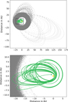 |
Fig. 1 Example of the orbit of a simulated test particle initiated with a = 25.73 AU. The grey points show the orbit computed during the low-resolution simulation. The particle initially undergoes interactions with β Pic b and reaches a periastron distance of less than 3 AU at some moment in the simulation. Then the resolution of the simulation is increased, resulting in the orbit shown in green. This high-resolution simulation ends when the periastron distance becomes less than 0.4 AU (marked with the green dot). |
2.2 Classification
During the simulation, a test particle was assigned a classification if it fulfilled a set of conditions. Firstly, a test particle would be classified as ejected if it was found to be on a hyperbolic orbit (i.e. had an eccentricity of e > 1) and located at a distance greater than 150 AU, a distance that is large compared to the orbits of the planets. Secondly, a particle could collide with one of the planets in the system. Collisions were evaluated using the REBOUND ‘line’ routine that linearly interpolates the positions of a particle between subsequent time steps (Rein & Liu 2012), following Rodet & Lai (2024). We tested the sensitivity of the results to the assumed size of the collision radii of the planets and this is presented in Appendix A. Finally, test particles were labelled as star-grazers if their periastron distance was below 0.4 AU. This limit is grounded in the work of Beust et al. (1998) who argued that this is the maximal distance at which dusty particles evaporate sufficiently to produce observable absorption. However, the particle was only classified as a star-grazer if its position was within 1 AU from the star. This additional criterion was necessary to make sure that the particle was no longer interacting with β Pic c, as close encounters with it could momentarily change the periastron distance within the 0.4 AU limit, potentially yielding false classifications. Any particle classified according to any of these three criteria was removed from the simulation and its final orbital elements at that simulation time were saved.
3 Results
We discuss the outcomes of the simulation in the sections below. Section 3.1 presents the classification of particles at the end of the simulation, establishing a comparison with Rodet & Lai (2024). Section 3.2 offers a discussion of the regions from where particles tend to migrate onto star-grazing orbits in the latter half of the simulation, taken to be representative for the time at the current age of the system. Section 3.3 evaluates the orbital characteristics of the particles at the moment that they are classified as star-grazers and derives their radial velocities when seen transiting the line of sight. Here, we find that our simulation produced two distinct dynamical families of exocomets. This is in line with the spectroscopic survey of Kiefer et al. (2014) that demonstrates the existence of two exocomet populations based in part on their separate distributions of observed radial velocities. We therefore propose that the different dynamical families presented by Kiefer et al. (2014) distinguish particles that originated within the orbits of the planets from those that originated beyond the orbits of the planets. Section 3.5 covers the possible implications for the compositions of the exocomets, as both populations may have been devolatilised to different degrees.
3.1 Branching ratios
Figure 2 shows the relative frequencies (branching ratios) of the classifications of particles at the end of the simulation (see Sect. 2.2). Figure 2 is cut off at an orbital distance of 35 AU, while the simulated disc extends to 45 AU, where all particles remain stable. Our branching ratios are broadly consistent with those presented by Rodet & Lai (2024, shown in their Fig. 19), in that the majority of particles below 35 AU are ejected, while the remainder become star-grazing or collide with a planet. We simulated the system with a higher number of particles than Rodet & Lai (2024) to allow for a higher resolving power in the semimajor axis distribution and this reproduces key properties of the evolution already seen in Fig. 19 of Rodet & Lai (2024) as well as Fig. 3 of Beust et al. (2024). The existence of a region beyond ~35 AU where the vast majority of particles survive for the duration of the simulation (we refer to this as a ‘stable’ region), as well as regions between 20 and 25 AU, where most particles are dynamically cleared within 25 Myr, but a small number on the order of ~10% remains. 15% of all particles initialised at orbits within 35 AU ultimately evolve to pass within 0.4 AU of the star, and are classified as a star-grazer at some moment in the simulation. The fraction of particles that does so increases from 5.8% for particles initialised between 20 and 25 AU up to 55% of particles initialised on orbits within 3 AU. The differences between our simulation and that of Rodet & Lai (2024) are that our star-grazer criterion is slightly more inclusive at 0.4 AU versus 0.3 AU of Rodet & Lai (2024), and that our simulation runs for 25 Myr instead of 10 Myr, which can explain why we find our outer stable region at a larger distance from the star: at later simulation times, the regions between 20 and 25 AU and beyond 35 AU, where significant fractions of particles survived are progressively eroded. As we show here, this erosion is a plausible source for ongoing exocomet creation at the age of the system. Besides star-grazers, the vast majority of particles, 75% are ejected from the system (light and dark blue in Fig. 2). Of all the planetesimals that are initiated within 35 AU, about 1% of them are expected to collide with either of the planets.
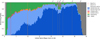 |
Fig. 2 Branching ratios of the entire initial particle population, up to 35 AU after running the simulation (see our methods in Sect. 2) for 25 million years. Throughout the system, the majority of particles are ejected (blue) up to a distance of ∼35 AU, beyond which particles are stable over the system’s lifetime. Particles that are ejected without attaining an orbit that passes within the 3 AU limit (i.e. they are only ever simulated using the lower resolution time step before being ejected) are shown in dark blue. However, many particles from the outer system pass within the 3 AU boundary and are also simulated using the high-resolution time step before being ejected (light blue). All particles initiated on orbital distance smaller than 3 AU are always simulated in high-resolution and, thus, also shown in light blue if ejected. A significant number of particles approach the star to within 0.4 AU, which we classify as star-grazers (green). A small number of particles collides with either of the planets. This figure is comparable with the simulation output of Rodet & Lai (2024, their Fig. 19). |
3.2 The formation of exocomets at late times
Although our branching ratios are in line with a previous work (Rodet & Lai 2024), we note that branching ratios only show the ultimate outcome of all particles in the simulation, without any information about the time. Therefore, branching ratios do not make evident how star-grazer creation changes during the system’s evolution, nor do they show the distribution of star-grazers and ejections being created at the present-day time. Branching ratios also depend on the choice of start and end times of the classification, in our case ranging from 0 to 25 million years2. Therefore, we also show this classification as a function time in Fig. 3. From these figures, it is apparent that the majority of the system within 35 AU is unstable to perturbations by the planets on relatively short (< 105 yr) timescales, as is well known (Rodet & Lai 2024; Beust et al. 2024). Most of the classified star-grazers thus become star-grazing very early on in the system’s lifetime and these particles are not related to the exocomet phenomenon observed at the present time. However, even after millions of years after the clearing of these inner regions, we find that the creation of star-grazers can continue from three main regions, as seen in the right-most panel of Fig. 3, namely:
the inner edge of the outer stability region close to 35 AU, which moves outwards over time;
the intermediate stability regions between 20 to 25 AU that are demarcated by resonances with the orbital period of planet b;
the region within 1.5 AU.
To investigate the creation of star-grazers at late times in more detail, we went on to select only the particles classified as star-grazers at times greater than 10 Myr from the start of the simulation, which are 399 particles out of a grand total of 133 500. We refer to these as ‘late star-grazers’. These particles originate from the three main regions listed above; however for the sake of simplicity, we divide these into two main groups of late star-grazer origin: the inner region, which sources the stargrazers produced from the 1.5 AU stability region, and the outer region, which sources late star-grazers from both the intermediate stability regions between 20 and 25 AU, as well as the erosion of the disc beyond ~35 AU. As shown in Fig. 3, about 52% of late star-grazers (208) originate in the outer system, while a similar number of them (191) originate closer to the star. The rates of late star-grazer creation from the inner and outer regions are shown in Fig. 4. Here, the fraction of particles that stargraze at a given time is normalised to the total number of late star-grazers in each of the two regions. As expected, there is a declining rate of stargrazers being created from both regions over the last 15 million years of the simulation.
Intuitively, these numbers suggest that the rate of star-grazer formation is roughly equally split between the inner and outer regions; however, the relative sizes of these star-grazer populations are dependent on the number of particles initialised in each of these regions. As we distributed the particles uniformly in orbital distance (see more on our methods in Sect. 2), the relative rates at which star-grazers are formed cannot be directly inferred from these statistics. We therefore do not derive any conclusions about the absolute number of star-grazer formation, nor the relative rates between the inner and outer populations, besides the observation that the outer region is a plausible source of star-grazers at late times, in addition to the inner region that was already known (Beust et al. 2024).
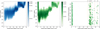 |
Fig. 3 Time dependence of the evolution of test particles. The two left-most panels show the survival times of particles that get ejected (left-most) or are star-grazing (middle), as a function of the initial semi-major axis at which the particles are seeded. The percentage of all simulated particles that is removed from the simulation is indicated with the colourbar. The right-most panel shows particles that become classified as star-grazing after 10 million years. We call these ‘late star-grazers’ and investigate them in further detail in Sect. 3.2. Note: there seem to be two different sources of late star-grazers, in the inner and outer parts of the system, respectively. Orbital resonances with β Pic b are also indicated such as in Fig. 2, clearly showing that star-grazers are not expected to be produced from low-order resonances (e.g. 1:3 and 1:4) because these have been cleared earlier in the life of the system. |
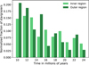 |
Fig. 4 The fraction of particles star-grazing at simulation times greater than 10 million years, normalised by the total number of late star-grazers from each respective region. The rate of star-grazers from both regions is decreasing over time at a similar rate. |
3.3 Two families of exocomets?
One of the primary observables from decades of spectroscopic monitoring has been the distribution of radial velocities of the exocomet population, which holds clues to their dynamical evolution (Kiefer et al. 2014). We therefore wish to predict the emergent radial velocity distribution of transiting exocomets generated in our simulation. In particular, we wish to confirm that the inner population is excited via mean-motion resonance with β Pic c, as predicted by Beust & Morbidelli (1996) and recently explored in more detail by Beust et al. (2024). Both of these objectives are complicated by the fact that the orbit of β Pic c precesses rapidly, with a period of approximately 10 000 years (Beust et al. 2024). This effectively rotates the directionality of the excitation phenomenon caused by mean-motion resonances (see Fig. 9 in Beust et al. 2024). In Beust et al. (2024), this was not considered to be a problem because these authors were still able to simulate a much larger number of particles thanks to their use of a symplectic integrator. We only created 399 exocomets and, thus, we did not have the ability to evaluate the statistics of the population at any particular phase of the precession of β Pic c (i.e. the present time).
However, assuming that the generation of exocomets is indeed dominated by interactions with β Pic c, we evaluated the relative orbital alignment of the exocomet populations, compared to the phase of rotation of the semi-major axis of β Pic c. We defined the angle, ∆ω = ω - ωc, as the difference between the argument of periastron of a star-grazing particle and the argument of periastron of β Pic c at the time when the particle is identified as a star-grazer the moment it crosses the threshold of 0.4 AU. In defining orbital elements, we used the convention by Green (1985), which was also used by Lacour et al. (2021), who compiled the system properties we adopted in this study (see Table 1). We defined a line of sight and a reference plane perpendicular to it. In this coordinate system, one principle axis is along the line of sight and one principle axis is along the angular momentum vector of the orbit of β Pic c. This means that at the start of the simulation, β Pic c obtains an inclination of 88.95°, as observed (Lacour et al. 2021), but the position angle of the ascending node Ωc is equal to zero3. For each star-grazing particle, we can then rotate the Euclidean coordinate frame of the simulation by an angle angle equal to ∆ω, such that at the epoch of star-grazer creation, the orbit of β Pic c is aligned with its orientation on the present day. This allows us to compare the alignment of star-grazing particles regardless of when they are created in the simulation.
Figure 5 shows the values of ∆ω of the exocomets originating from both the inner and the outer regions (see Sect. 3.2). This reveals that the inner population is indeed systematically excited in the direction aligned with the orbital semi-major axis of β Pic c, as expected from the mean-motion resonance effect.
Therefore, we can confirm the results from Beust et al. (2024); namely, that mean-motion resonances with β Pic c are capable of generating a distinct dynamical family of exocomets with very similar orbital parameters, thereby explaining the observed preferred redshift of the exocomet population. Interestingly, we find that there is also a notable alignment of the orbits of the population of exocomets that originally originate from the outer regions. Intuitively, these may be expected to arrive in the inner system on orbits that are random with respect to the orbit of β Pic c, but interactions with β Pic c do impart a preferential value for the argument of periastron, ω.
Having obtained the orbital configuration relative to the present-day orbit of β Pic c, we proceeded to evaluate the radial velocities of the populations during transit. However, star-grazers have non-zero inclinations with respect to the line of sight; thus, in principle, this might only be possible for a small fraction of particles because many may not transit. The left-most panel of Fig. 6 shows the distributions of the inclinations of both the inner and outer populations. The population of particles from the inner region has relatively small4 inclinations and we find that approximately a quarter of them indeed transit. Particles from the outer region have a larger spread of inclinations and only a small fraction (approximately 2%) transit. To obtain statistically meaningful samples of radial velocities for both populations, we opted to include particles with impact parameters greater than one. This is done by evaluating the velocity in the direction of the star ( ), effectively rotating the line of sight out of the plane to avoid biasing the velocity distribution to smaller values for particles that cross the transit centre plane at a large angle. For the particles from the inner region, this creates a negligible bias because the inclinations of the particles are within a few degrees. For the particles in the outer region, including these inclined particles could introduce a bias in the distribution of their radial velocities, but we found that including only low-inclination particles from this population does not significantly change the shape of the distribution (see Fig. B.1). We note that the large spread of inclinations of exocomets that originated from the outer system implies that the edge-on geometry of the β Pic system is not a requirement for observing the exocomet phenomenon. Thus, planetesimal discs with significant inclinations might still produce significant exocomet activity.
The resulting distributions of mid-transit radial velocities are shown in Fig. 7. The population from the inner region has a narrowly distributed radial velocity that is preferentially redshifted to a mean of 13 km/s with a standard deviation of 4 km/s. The population of particles from the outer regions results in a wider spread of radial velocities. These results are consistent with the observations of Kiefer et al. (2014), who found that exocomets can be distinguished into two dynamical families, based on their radial velocities, transit depths, and surface fill fractions. The average radial velocity of inner region particles in our simulation of 13 km/s is consistent with their observed value of 15 ± 6 km/s, as well as with the simulation results by Beust et al. (2024).
Figure 6 also shows the transverse velocities and resulting transit durations (assuming an average impact parameter of 0.5) derived in a similar manner as the radial velocities. We find that transits of both populations typically last for approximately 18 hours, explaining why spectra obtained during a single night tend to appear stable (Kiefer et al. 2014), apart from a small fraction that are observed to accelerate during transit (Kennedy 2018; Hoeijmakers et al. 2025). Transverse velocities of the particles from the inner region peak at approximately 30 km/s and are cut off below 20 km/s. The existence of a lower bound to the transverse velocity is expected because the population of inner particles is confined to a maximum orbital distance that coincides with the inner boundary of the instability region caused by β Pic c. Particles from the outer region have a wider range of transverse velocities and this is expected because they enter the inner system on a diverse range of orbits. Their distribution peaks at approximately 10 km/s, as these are particles that generally tend to have larger semi-major axes (see Fig. 5). The deep transit event observed by Zieba et al. (2019) allowed for a direct measurement of the transverse velocity of 19.6 ± 0.1 km/s, slightly below the cut-off velocity of the inner population of particles in our simulation. This could indicate that this was a particle originally originating from the outer region.
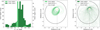 |
Fig. 5 Orbital alignment of the two exocomet populations. The left-most panel shows the difference between the argument of periastron of the test particle, ω, and the argument of periastron of β Pic c, ωc. The two panels to the right show the orbits of star-grazing test particles originating from the inner and outer exocomet reservoirs, respectively. The dashed line indicates the direction of the line of sight, while the plane of the sky is parallel to the horizontal axis. Note: in this projection of the coordinate system, particles generally orbit in a counter clock-wise direction. |
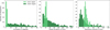 |
Fig. 6 Distributions of exocomet properties for the two identified families. The left-most panel shows the inclination from edge on orbit (90° − i). Note: this panel shows inclinations up to 60°, leaving out approximately 13% of particles from the outer region with higher inclinations. The middle panel shows the transit duration up to 150 hours (assuming an average impact parameter of 0.5), leaving out approximately 4% of particles from the outer region with longer transit durations. Finally the right-most panel shows the transverse velocity. |
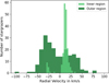 |
Fig. 7 Radial velocity distributions of the two exocomet families. Exocomets originating in the inner region mostly occur in a narrow distribution of radial velocities with a centre of 13 km/s and standard deviation of 4 km/s. Exocomets from the outer region have a broader distribution of radial velocities. |
3.4 Simulation limitations
Although our simulation seems to accurately reproduce the radial velocity distribution observed for the population of meanmotion resonance exocomets (Kiefer et al. 2014; Beust et al. 2024), the wider distribution of the particles originating in the outer system does not exactly match observations, as there appear to be more blueshifted particles in our results. We point out four important caveats that arise from choices made in our simulation and analysis, which could affect the shape of the distribution of this population in particular.
Firstly, our simulation results are applicable to star-grazers on orbits for which the periastron distance has crossed 0.4 AU for the first time. Thus, our simulation does not capture further orbital evolution that could lead to orbits getting closer the star. This would generally allow for faster exocomets and this also explains why the broad distribution of particles originating from the outer system is limited to radial velocities of ±50 km/s; whereas in reality, much higher radial velocities have also been observed (Kiefer et al. 2014). Intuitively, we predict that continued orbital evolution of inner region exocomets will be less pronounced than those from the outer regions, as the latter interact more chaotically with β Pic c. Conversely, it may also be possible that exocomets already become visible when their periastron is further away than 0.4 AU from the star, potentially leading to a lower cut-off value for the transverse velocity of the inner population (Fig. 5).
Secondly, we note that our simulation counts numbers of star-grazing particles. We did not model the possibility that a single exocomet can be observed to transit many times or that a single particle could break up into a population of particles on similar orbits (Beust et al. 1996); this would be required for a reliable comparison between our velocity distributions and those seen in observations. Doing so would require accurate modelling of tidal break-up, as well as the disappearance of exocomets due to sublimation, and such results would be highly model-dependent. However, we do expect the distribution of the exocomets from the inner system to be largely robust because the population of orbits is very coherent.
Thirdly, we note that a roughly equal number of exocomets originated from either region in our simulation, but that this does not imply that our simulation predicts that these regions would be realistically expected to source star-grazers at a relatively equal rate. Our simulation was initialised with an arbitrary density of seed particles that might not match the density distribution of particles in the primordial β Pic planetesimal disc. Furthermore, particles arriving from the outer region to the inner region obtain a larger spread of inclinations than the particles that originate from the inner region (Fig. 6), meaning that a smaller number of particles from the outer system become observable as transiting exocomets. Interpreting the observed relative numbers of particles in both populations requires these effects to be robustly taken into account, but this is presently complicated by the first and second caveats already mentioned above.
Fourthly, in correcting for the effect of β Pic c’s precessing orbit, we rotated the coordinate frame for all star-grazing particles to match β Pic c’s current orbit. If β Pic b were to impart any preferred directionality to the orbits of the exocomet population, this would be washed out. However, we note that β Pic b has a much smaller eccentricity and this would only affect the population of exocomets coming from the outer regions.
One final note is that our simulation currently uses the IAS15 integrator, although a new hybrid symplectic integrator TRACE was released (Lu et al. 2024) during the preparation of the current paper. TRACE is designed to handle close encounters by dynamically switching to non-symplectic integration when needed, while maintaining high-speed symplectic integration for particles not undergoing close encounters. In theory, implementing TRACE for the β Pic system could allow for significant increases in simulation speed and, therefore, a larger number of simulated particles.
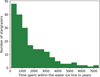 |
Fig. 8 Amount of time that exocomets from the outer region spend inside the water ice line (estimated to lie at 8.2 AU), while migrating toward the vicinity of the star before being classified as an exocomet. All these particles originate outside of the water ice line of the β Pic system (see Fig. 3). |
3.5 Implications for exocomet composition
Exocomets are primarily observed via the strong Ca II H&K lines that are the result of photoionisation of sublimated refractory dust when the planetesimal is very close to the star. A key question has been whether the transiting exocomets are dominated by volatiles or are mostly rocky (Beust et al. 1989; Beust et al. 1990; Wilson et al. 2017; Beust et al. 2024; Kenworthy et al. 2025). Calcium is sublimated from refractory material on the exocomet surface, but it could be part of a volatile-rich outflow that is spectroscopically invisible. Past models of exocomet cloud morphology have assumed icy compositions for the evaporating exocomets, resulting in volatile-rich outflows (e.g. Kiefer et al. 2014).
In our simulation, the exocomet progenitors from the outer region originate at orbital distances much beyond the water ice line located at approximately 8 AU, as determined by matching the sublimation temperature (Lodders 2003) to the equilibrium temperature in the β Pic system. We find that exocomet progenitors that get perturbed to become exocomets, typically spending 102 to 103 years within a distance of 8 AU before finally being identified as exocomet candidates at a distance of 0.4 AU (see Fig. 8). Karmann et al. (2001) systematically modelled the sublimation of ice-dominated exocomet progenitors, based on orbital distance, nucleus size, and ice content. For ice contained in porous rocky bodies, they found that ice could potentially survive for > 105 years in 1 km-sized bodies at orbital distances closer than 5 AU from the star (Fig. 7 in Karmann et al. 2001). We therefore conclude that exocomets originating from the outer system may have retained significant fractions of ice, which could influence their outgassing characteristics and outgassing composition.
We note that Kiefer et al. (2014) already observed systematic differences in cloud morphologies between the two populations. The comets with a wide distribution of radial velocities (S family) tend to have small fill fractions of the stellar disc. Kiefer et al. (2014) interpreted the orbital characteristics of this population to be consistent with mean-motion resonance and that the small fill fraction is caused by a lower evaporation rate, consistent with the expectation that such a population would be devolatilised. However, Kiefer et al. (2014) predates the discovery of β Pic c, and more recent simulations by Beust et al. (2024), also supported in the present study, indicate that the other population, with a narrow radial velocity distribution (D family), is in mean-motion resonance with β Pic c instead. Kiefer et al. (2014) proposed that the D family is volatile-rich, but our simulations as well as the simulations of Beust et al. (2024) posit that this population has been located interior to the orbit of β Pic c for millions of years. This means that they are expected to be primordially devolatilised - unless the rocky material was highly carbonaceous (Karmann et al. 2001; Fernández et al. 2006; Beust et al. 2024). A recent study (Vrignaud & Lecavelier des Etangs 2026), using measurements of the population levels of exocomet cloud species, found that several exocomets associated with family D transit at significantly larger distances than previously assumed, such as the example present in Kiefer et al. (2014). This is consistent with our simulations that predict that in-transit distances of up to 1.5 AU are expected for the population in mean-motion resonance (see Fig. 5), although one object identified by Vrignaud & Lecavelier des Etangs (2026) transits at a distance of almost 5 AU from the star. Our simulation does not predict any exocomets from the population in mean-motion resonance to reach such large distances, implying that this object is expected to have originated from the regions beyond the orbit of β Pic b.
Our results suggest that the population of comets with a broad radial velocity distribution (S family) originates from the outer system and may hence be richer in volatiles. Further modelling of outgassing processes and cloud dynamics are required to coherently explain the observed cloud properties with these dynamical evolution scenarios. We propose that spectroscopic observations may be capable of probing differences in the volatile contents between these populations. It has been observed and proposed that atomic hydrogen might be produced via water ice evaporation of infalling exocomets (Wilson et al. 2017). An initial attempt to discover cynaogen (CN) was recently undertaken by Kenworthy et al. (2025).
4 Conclusions
We carried out a sequence of dynamical simulations of over 100000 particles in the β Pic system using REBOUND to explore the dynamical origins of exocomets observed via spectroscopy and photometry (Ferlet et al. 1987; Kiefer et al. 2014; Zieba et al. 2019). We assumed a flat disc (i = ±2°) of mass-less test particles initiated on near-circular orbits with semi-major axes between 0.5 and 45 AU and integrated these with the high-accuracy IAS15 integrator for a period of 25 Myr equivalent to the age of the system. We found that a small fraction of particles may be evolved onto star-grazing orbits, originating from two main regions: within and exterior to the orbits of the two planets.
Particles from the outer system gradually become excited by interactions with β Pic b, until they experience close encounters. A fraction of these particles is scattered towards the inner system, interacting chaotically with both planets until some reach highly elliptical, star-grazing orbits. In addition, we find that a significant fraction of 24% of all particles originating from within 1.5 AU remain stable for the lifetime of the system. Furthermore, particles from within this inner population exhibit mean-motion resonances with β Pic c, which coherently excite their orbits until they star-graze. This phenomenon has been investigated in detail by Beust et al. (2024), who have proposed this to be the explanation for the exocomet phenomenon observed in β Pic since the 1980’s (Ferlet et al. 1987).
We can now conclude that particles from both the inner and the outer regions have the potential to dynamically evolve to become exocomets. Evaluating the relevant orbital parameters and radial velocities reveals that both populations have distinct dynamical properties: Star-grazers from within the orbit of β Pic c that are excited via MMR display a narrow radial velocity distribution centred on 13 ± 4 km/s that is consistent with the simulation results of Beust et al. (2024), which reproduces the observed narrow radial velocity distribution of one observed family of exocomets by Kiefer et al. (2014) that is centred at 15 ± 6 km/s. We also find that the star-grazers that originate from beyond the orbit of β Pic b enter the inner system on more chaotic orbits, resulting in a broad distribution of radial velocities. We infer that this could explain the population that has been spectroscopically observed to have a broad velocity distribution (Kiefer et al. 2014). The population of star-grazers from the outer regions might have retained significant volatile reservoirs, which could explain the differences in cloud morphology that have been observed spectroscopically (Kiefer et al. 2014), and distinct spectroscopic signatures due to volatile outgassing may be observable for these exocomets. Interestingly, gaseous exocometary clouds were recently observed at transit distances of up to almost 5 AU (Vrignaud & Lecavelier des Etangs 2026). We also find that exocomets originating from the outer region obtain a large spread of orbital inclinations, meaning that exocomets may be expected to be observable in planetesimal discs that are not viewed edge-on, as in the case of β Pictoris.
An important limitation of our simulation is represented by the main criterion used to identify star-grazers, historically defined via an orbital distance criterion of 0.4 AU (e.g. Beust et al. 2024), which might be inaccurate. Moreover, our particles have been classified as star-grazers only once and this neglects the possibility of the same particle transiting multiple times or streams of particles that result from tidal break-up, which is likely to be an important effect (Beust et al. 1996). Finally, our prediction for the number of star-grazers depends strongly on the assumed number of particles initialised in the simulation, making the number of particles generated relative to the unknown size of the real particle reservoir.
Acknowledgements
This work was supported by grants from eSSENCE (grant number eSSENCE@LU 9:3), the Swedish National Research Council (project number 2023-05307), The Crafoord foundation and the Royal Physiographic Society of Lund, through The Fund of the Walter Gyllenberg Foundation. We are grateful to Bibiana Prinoth for important discussions regarding sky-projected orbital elements. We also thank an anonymous referee for their insightful and detailed comments that helped us significantly improve the manuscript.
References
- Aumann, H. H. 1985, PASP, 97, 885 [Google Scholar]
- Beust, H., & Morbidelli, A. 1996, Icarus, 120, 358 [NASA ADS] [CrossRef] [Google Scholar]
- Beust, H., Lagrange-Henri, A., Vidal-Madjar, A., & Ferlet, R. 1989, A&A, 223, 304 [NASA ADS] [Google Scholar]
- Beust, H., Lagrange-Henri, A. M., Vidal-Madjar, A., & Ferlet, R. 1990, A&A, 236, 202 [NASA ADS] [Google Scholar]
- Beust, H., Lagrange, A.-M., Plazy, F., & Mouillet, D. 1996, A&A, 310, 181 [Google Scholar]
- Beust, H., Lagrange, A. M., Crawford, I. A., et al. 1998, A&A, 338, 1015 [NASA ADS] [Google Scholar]
- Beust, H., Milli, J., Morbidelli, A., et al. 2024, A&A, 683, A89 [NASA ADS] [CrossRef] [EDP Sciences] [Google Scholar]
- Blunt, S., Wang, J. J., Angelo, I., et al. 2020, AJ, 159, 89 [NASA ADS] [CrossRef] [Google Scholar]
- Burrows, C. J., Krist, J. E., Stapelfeldt, K. R., & WFPC2 Investigation Definition Team. 1995, in American Astronomical Society Meeting Abstracts, 187, 32.05 [NASA ADS] [Google Scholar]
- Chambers, J. E. 1999, MNRAS, 304, 793 [Google Scholar]
- Chauvin, G., Lagrange, A. M., Beust, H., et al. 2012, A&A, 542, A41 [NASA ADS] [CrossRef] [EDP Sciences] [Google Scholar]
- Chen, C. H., Lu, C. X., Worthen, K., et al. 2024, ApJ, 973, 139 [Google Scholar]
- Crifo, F., Vidal-Madjar, A., Lallement, R., Ferlet, R., & Gerbaldi, M. 1997, A&A, 320, L29 [NASA ADS] [Google Scholar]
- Di Folco, E., Thévenin, F., Kervella, P., et al. 2004, A&A, 426, 601 [NASA ADS] [CrossRef] [EDP Sciences] [Google Scholar]
- Edlén, B., & Risberg, P. 1956, Ark. Fys., 10, 553 [Google Scholar]
- Ferlet, R., Hobbs, L. M., & Vidal-Madjar, A. 1987, A&A, 185, 267 [NASA ADS] [Google Scholar]
- Fernández, R., Brandeker, A., & Wu, Y. 2006, ApJ, 643, 509 [CrossRef] [Google Scholar]
- Golimowski, D. A., Ardila, D. R., Krist, J. E., et al. 2006, AJ, 131, 3109 [NASA ADS] [CrossRef] [Google Scholar]
- GRAVITY Collaboration (Nowak, M., et al.) 2020, A&A, 633, A110 [NASA ADS] [CrossRef] [EDP Sciences] [Google Scholar]
- Green, R. M. 1985, Spherical Astronomy (Cambridge University Press) [Google Scholar]
- Hobbs, L. M., Vidal-Madjar, A., Ferlet, R., Albert, C. E., & Gry, C. 1985, ApJ, 293, L29 [NASA ADS] [CrossRef] [Google Scholar]
- Hoeijmakers, H. J., Jaworska, K. P., & Prinoth, B. 2025, A&A, 700, A239 [NASA ADS] [CrossRef] [EDP Sciences] [Google Scholar]
- Kammerer, J., Lawson, K., Perrin, M. D., et al. 2024, AJ, 168, 51 [NASA ADS] [CrossRef] [Google Scholar]
- Karmann, C., Beust, H., & Klinger, J. 2001, A&A, 372, 616 [NASA ADS] [CrossRef] [EDP Sciences] [Google Scholar]
- Kennedy, G. M. 2018, MNRAS, 479, 1997 [NASA ADS] [CrossRef] [Google Scholar]
- Kenworthy, M. A., de Mooij, E., Brandeker, A., et al. 2025, A&A, 698, A10 [NASA ADS] [CrossRef] [EDP Sciences] [Google Scholar]
- Kiefer, F., Lecavelier des Etangs, A., Boissier, J., et al. 2014, Nature, 514, 462 [Google Scholar]
- Lacour, S., Wang, J. J., Rodet, L., et al. 2021, A&A, 654, L2 [NASA ADS] [CrossRef] [EDP Sciences] [Google Scholar]
- Lagrange, A. M., Bonnefoy, M., Chauvin, G., et al. 2010, Science, 329, 57 [Google Scholar]
- Lagrange, A. M., Meunier, N., Rubini, P., et al. 2019, Nat. Astron., 3, 1135 [NASA ADS] [CrossRef] [Google Scholar]
- Lagrange-Henri, A. M., Vidal-Madjar, A., & Ferlet, R. 1988, A&A, 190, 275 [NASA ADS] [Google Scholar]
- Lodders, K. 2003, ApJ, 591, 1220 [Google Scholar]
- Lu, T., Hernandez, D. M., & Rein, H. 2024, MNRAS, 533, 3708 [Google Scholar]
- Mamajek, E. E., & Bell, C. P. M. 2014, MNRAS, 445, 2169 [Google Scholar]
- Mouillet, D., Larwood, J. D., Papaloizou, J. C. B., & Lagrange, A. M. 1997, MNRAS, 292, 896 [Google Scholar]
- Nowak, M., Lacour, S., Lagrange, A. M., et al. 2020, A&A, 642, L2 [NASA ADS] [CrossRef] [EDP Sciences] [Google Scholar]
- Ravet, M., Bonnefoy, M., Chauvin, G., et al. 2025, A&A, 704, A325 [NASA ADS] [CrossRef] [EDP Sciences] [Google Scholar]
- Rein, H., & Liu, S. F. 2012, A&A, 537, A128 [NASA ADS] [CrossRef] [EDP Sciences] [Google Scholar]
- Rein, H., & Spiegel, D. S. 2015, MNRAS, 446, 1424 [Google Scholar]
- Rodet, L., & Lai, D. 2024, MNRAS, 527, 11664 [Google Scholar]
- Slettebak, A., & Carpenter, K. G. 1983, ApJS, 53, 869 [Google Scholar]
- Smith, B. A., & Terrile, R. J. 1984, Science, 226, 1421 [Google Scholar]
- Vrignaud, T., & Lecavelier des Etangs, A. 2026, A&A, 707, A60 [NASA ADS] [CrossRef] [EDP Sciences] [Google Scholar]
- Wilson, P. A., Lecavelier des Etangs, A., Vidal-Madjar, A., et al. 2017, A&A, 599, A75 [NASA ADS] [CrossRef] [EDP Sciences] [Google Scholar]
- Worthen, K., Chen, C. H., Law, D. R., et al. 2024, ApJ, 964, 168 [NASA ADS] [CrossRef] [Google Scholar]
- Yoshikawa, M. 1989, A&A, 213, 436 [NASA ADS] [Google Scholar]
- Zieba, S., Zwintz, K., Kenworthy, M. A., & Kennedy, G. M. 2019, A&A, 625, L13 [NASA ADS] [CrossRef] [EDP Sciences] [Google Scholar]
In theory, mass-less test particles do not influence one another. However in REBOUND, the simulation time step is adaptive, depending on the proximity of particles to massive particles. This means that removing or adding mass-less particles to a simulation does influence the global outcome, even of the massive particles. This means that two simulations of the same system with different test particles will diverge, despite the fact that test particles do not explicitly exert forces on the massive particles.
This means that particles classified as stable are to be understood to be stable only for the 25 million year duration of the simulation – and not necessarily in the future. Grey areas in the branching ratios (Fig. 2) might be referred to as stability regions, but this is only valid within the 25 million year time frame.
Our reference plane effectively points 31.05° away from North in the sky.
For simplicity, we refer to nearly edge-on orbits as having a small inclination. However, the orbital element i is defined to be 90° for edgeon orbits, so the quantity that is referred to as small is actually 90°−i.
Appendix A Sensitivity tests
We carried out two tests to determine how our results are influenced by choices of initial conditions. First, we tested how the choice of radii of β Pic b and c affect the rate at which particles are predicted to collide with either of the planets, and thereby the branching ratios and creation of star-grazers at late times. The region between 23 and 24 AU was chosen for this test, as it is a region where all the fates of test particles are possible, see Fig. 2. The majority of particles in this region are ejected; however, a smaller fraction stargraze, collide with either of the planets or remain stable for the full duration of the simulation. Of particular interest is whether the number of late star-grazers from this region is significantly affected by the choice of planet radii.
We simulated the region between 23 and 24 AU using planetary radii that are twice as large as the ones used in the original simulation, presented in Sect. 2.1. The resulting branching ratios are shown in the middle panel of Fig. A.1. From this sensitivity test we conclude that large changes in the radii of the planets do not significantly alter the results of the simulation: The fraction of colliding particles increases by 70% and the fraction of particles that remain stable decreases by 11%. Importantly, the number of late star-grazers only decreases by one singular late star-grazer, 85 late star-grazers were produced in this region in the original simulation using the nominal radii, and 84 in the test simulation where the radii were doubled. This implies that our uncertainty about the true effective collision radius of the planets, does not meaningfully affect the statistics of the stargazing populations that we present in our conclusions.
Furthermore, we preformed a test of the sensitivity of the choice of a maximal time step using the same range of distances of 23 - 24 AU. Here, this region was simulated using the high-resolution time step, that was otherwise only used for particles that cross the 3 AU threshold (see Sect. 2.1). The resulting branching ratios are shown in the right-most panel of Fig. A.1. In this simulation, the total number of star-grazing particles decreases by 3% and the total number of stable particles increases by 6% relative to the original simulation. The number of late star-grazers from this region is 75 for the highresolution test, compared to 85 late star-grazers produced in this region by the original simulation set-up, as described in Sect. 2.1. From this, we conclude that switching the time-resolution does not strongly alter the distribution of outcomes of our simulations, sufficient to violate the conclusion that the particles from regions beyond the orbit of β Pic b constitute a plausible source of star-grazers at the age of the system.
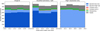 |
Fig. A.1 Branching ratios of the region between 23 and 24 AU. The left-most panel shows a zoom-in of Fig. 2, where the simulation was performed using the same set-up as the one presented in Sect. 2.1. The middle panel shows the resulting branching ratios of the same region from a simulation where the planetary radii used were doubled. Similarly, the right-most panel shows the branching ratios of this region resulting from a simulation following the set-up as described in Sect. 2.1, but in which all particles were simulated using only the high-resolution time step. |
Appendix B Radial velocity distributions of exocomets with different inclinations
Our radial velocity distributions shown in Fig. 7 include particles with impact parameters larger than one (see Sect. 3.3). As discussed in Sect. 3.3, this inclusion of inclined star-grazers could introduce a bias to the radial velocity distribution. We test this by limiting the inclinations of the star-grazing particles and compare the radial velocity distributions in Fig. B.1. The top panel shows the radial velocity distribution of late star-grazers from the outer population. In green, all late star-grazers are included. In the distributions coloured purple, only star-grazers on orbits inclined by less than 60° (dark purple) and 20° (light purple) are included. Similarly, the bottom panel shows the radial velocity distributions of all inner population late star-grazers (green), star-grazers on orbits with inclinations smaller than 2° (dark pink), and transiting particles (light pink). From Fig. B.1, we can conclude that the larger inclinations of late star-grazers do not bias the radial velocity distributions and our conclusions are robust against this.
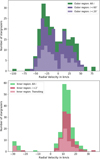 |
Fig. B.1 Radial velocity distributions of the inner and outer regions for different inclination limits. |
All Tables
Two recent solutions of parameters of the β Pic system: Solution 1 by Lacour et al. (2021) and solution 2 by Blunt et al. (2020) reproduced from Beust et al. (2024).
Initial conditions of the simulated disc of test particles modelling planetesimals.
All Figures
|
Fig. 1 Example of the orbit of a simulated test particle initiated with a = 25.73 AU. The grey points show the orbit computed during the low-resolution simulation. The particle initially undergoes interactions with β Pic b and reaches a periastron distance of less than 3 AU at some moment in the simulation. Then the resolution of the simulation is increased, resulting in the orbit shown in green. This high-resolution simulation ends when the periastron distance becomes less than 0.4 AU (marked with the green dot). |
| In the text | |
|
Fig. 2 Branching ratios of the entire initial particle population, up to 35 AU after running the simulation (see our methods in Sect. 2) for 25 million years. Throughout the system, the majority of particles are ejected (blue) up to a distance of ∼35 AU, beyond which particles are stable over the system’s lifetime. Particles that are ejected without attaining an orbit that passes within the 3 AU limit (i.e. they are only ever simulated using the lower resolution time step before being ejected) are shown in dark blue. However, many particles from the outer system pass within the 3 AU boundary and are also simulated using the high-resolution time step before being ejected (light blue). All particles initiated on orbital distance smaller than 3 AU are always simulated in high-resolution and, thus, also shown in light blue if ejected. A significant number of particles approach the star to within 0.4 AU, which we classify as star-grazers (green). A small number of particles collides with either of the planets. This figure is comparable with the simulation output of Rodet & Lai (2024, their Fig. 19). |
| In the text | |
|
Fig. 3 Time dependence of the evolution of test particles. The two left-most panels show the survival times of particles that get ejected (left-most) or are star-grazing (middle), as a function of the initial semi-major axis at which the particles are seeded. The percentage of all simulated particles that is removed from the simulation is indicated with the colourbar. The right-most panel shows particles that become classified as star-grazing after 10 million years. We call these ‘late star-grazers’ and investigate them in further detail in Sect. 3.2. Note: there seem to be two different sources of late star-grazers, in the inner and outer parts of the system, respectively. Orbital resonances with β Pic b are also indicated such as in Fig. 2, clearly showing that star-grazers are not expected to be produced from low-order resonances (e.g. 1:3 and 1:4) because these have been cleared earlier in the life of the system. |
| In the text | |
|
Fig. 4 The fraction of particles star-grazing at simulation times greater than 10 million years, normalised by the total number of late star-grazers from each respective region. The rate of star-grazers from both regions is decreasing over time at a similar rate. |
| In the text | |
|
Fig. 5 Orbital alignment of the two exocomet populations. The left-most panel shows the difference between the argument of periastron of the test particle, ω, and the argument of periastron of β Pic c, ωc. The two panels to the right show the orbits of star-grazing test particles originating from the inner and outer exocomet reservoirs, respectively. The dashed line indicates the direction of the line of sight, while the plane of the sky is parallel to the horizontal axis. Note: in this projection of the coordinate system, particles generally orbit in a counter clock-wise direction. |
| In the text | |
|
Fig. 6 Distributions of exocomet properties for the two identified families. The left-most panel shows the inclination from edge on orbit (90° − i). Note: this panel shows inclinations up to 60°, leaving out approximately 13% of particles from the outer region with higher inclinations. The middle panel shows the transit duration up to 150 hours (assuming an average impact parameter of 0.5), leaving out approximately 4% of particles from the outer region with longer transit durations. Finally the right-most panel shows the transverse velocity. |
| In the text | |
|
Fig. 7 Radial velocity distributions of the two exocomet families. Exocomets originating in the inner region mostly occur in a narrow distribution of radial velocities with a centre of 13 km/s and standard deviation of 4 km/s. Exocomets from the outer region have a broader distribution of radial velocities. |
| In the text | |
|
Fig. 8 Amount of time that exocomets from the outer region spend inside the water ice line (estimated to lie at 8.2 AU), while migrating toward the vicinity of the star before being classified as an exocomet. All these particles originate outside of the water ice line of the β Pic system (see Fig. 3). |
| In the text | |
|
Fig. A.1 Branching ratios of the region between 23 and 24 AU. The left-most panel shows a zoom-in of Fig. 2, where the simulation was performed using the same set-up as the one presented in Sect. 2.1. The middle panel shows the resulting branching ratios of the same region from a simulation where the planetary radii used were doubled. Similarly, the right-most panel shows the branching ratios of this region resulting from a simulation following the set-up as described in Sect. 2.1, but in which all particles were simulated using only the high-resolution time step. |
| In the text | |
|
Fig. B.1 Radial velocity distributions of the inner and outer regions for different inclination limits. |
| In the text | |
Current usage metrics show cumulative count of Article Views (full-text article views including HTML views, PDF and ePub downloads, according to the available data) and Abstracts Views on Vision4Press platform.
Data correspond to usage on the plateform after 2015. The current usage metrics is available 48-96 hours after online publication and is updated daily on week days.
Initial download of the metrics may take a while.