| Issue |
A&A
Volume 708, April 2026
|
|
|---|---|---|
| Article Number | A94 | |
| Number of page(s) | 19 | |
| Section | Stellar structure and evolution | |
| DOI | https://doi.org/10.1051/0004-6361/202556184 | |
| Published online | 31 March 2026 | |
Discovery of energy-dependent phase variations in the polarization angle of Cen X-3
1
State Key Laboratory of Particle Astrophysics, Institute of High Energy Physics, Chinese Academy of Sciences, Beijing 100049, China
2
University of Chinese Academy of Sciences, Chinese Academy of Sciences, Beijing 100049, China
3
Department of Physics and Astronomy, FI-20014 University of Turku, Finland
4
Department of Astronomy, University of Geneva, 16 Chemin d’Ecogia, Versoix CH-1290, Switzerland
5
Astrophysics, Department of Physics, University of Oxford, Denys Wilkinson Building, Keble Road, Oxford OX1 3RH, UK
6
Mullard Space Science Laboratory, University College London, Holmbury St. Mary, Surrey RH5 6NT, UK
★ Corresponding authors: This email address is being protected from spambots. You need JavaScript enabled to view it.
; This email address is being protected from spambots. You need JavaScript enabled to view it.
Received:
30
June
2025
Accepted:
22
February
2026
Abstract
We present a detailed polarimetric analysis of Cen X-3 using IXPE observations during its high state, revealing a complex, energy-dependent polarization behavior. While phase-averaged polarization shows marginal energy dependence, phase-resolved analysis reveals that the energy dependence of the polarization angle is strongly phase-dependent, with dramatic variations visible in a few specific phase intervals. We modeled this behavior using a two-component polarization framework consisting of a pulsed component governed by the rotating vector model (RVM) and an additional phase-dependent component. By allowing the additional component’s polarized flux to vary with pulse phase while fixing its PA, the observed complex behavior can be reconciled with a single set of RVM parameters across all energies. Spectroscopic analysis using IXPE, NICER, and NuSTAR during the high state reveals phase-modulated intrinsic hydrogen column density and covering fraction, suggesting that the wind properties are modulated with pulse phase. Our findings indicate that phase-dependent scattering in the disk wind may significantly alter the observed polarization properties of X-ray pulsars.
Key words: magnetic fields / polarization / methods: observational / techniques: polarimetric / stars: neutron / X-rays: binaries
© The Authors 2026
 Open Access article, published by EDP Sciences, under the terms of the Creative Commons Attribution License (https://creativecommons.org/licenses/by/4.0), which permits unrestricted use, distribution, and reproduction in any medium, provided the original work is properly cited.
This article is published in open access under the Subscribe to Open model. This email address is being protected from spambots. You need JavaScript enabled to view it. to support open access publication.
1. Introduction
Accreting X-ray pulsars (XRPs) are binary systems consisting of strongly magnetized neutron stars, with dipole magnetic fields of 1012–1013 G, accreting material from a donor star. The interaction between strong magnetic fields, radiation, and accreting matter leads to the diverse and complex observational behavior of XRPs (see Mushtukov & Tsygankov 2024, for a recent review). These strong magnetic fields fundamentally alter underlying physical processes such as the Compton scattering cross section. Due to the significant difference in opacity between the ordinary (O) and extraordinary (X) modes in the highly magnetized plasma of XRPs, radiation was previously expected to be strongly polarized, with the polarization degree (PD) reaching ∼80% (Meszaros et al. 1988; Caiazzo & Heyl 2021). The launch of the Imaging X-ray Polarimetry Explorer (IXPE; Soffitta et al. 2021; Weisskopf et al. 2022) in December 2021 has provided new opportunities for testing the X-ray polarization properties predicted by theoretical models.
To date, more than a dozen XRPs have been observed by IXPE, including Her X-1 (Doroshenko et al. 2022; Garg et al. 2023; Zhao et al. 2024; Heyl et al. 2024), Cen X-3 (Tsygankov et al. 2022), GRO J1008−57 (Tsygankov et al. 2023), 4U 1626−67 (Marshall et al. 2022), X Persei (Mushtukov et al. 2023), Vela X-1 (Forsblom et al. 2023, 2025), EXO 2030+375 (Malacaria et al. 2023), GX 301−2 (Suleimanov et al. 2023), RX J0440.9+44331/LS V +44 17 (Doroshenko et al. 2023; Zhao et al. 2025), Swift J0243.6+6124 (Majumder et al. 2024; Poutanen et al. 2024), SMC X-1 (Forsblom et al. 2024), and 4U 1538−52 (Loktev et al. 2025). Surprisingly, all these sources exhibit PDs significantly below theoretical predictions, even in phase-resolved measurements. Most IXPE targets were observed below the critical luminosity at which the accretion geometry transitions between a surface hot spot and an accretion column (Basko & Sunyaev 1976). Only a few sources, including RX J0440.9+4431/LS V +44 17 and SMC X-1, were observed in the supercritical regime, but they also exhibited low PDs. Another source, 1A 0535+262, observed by PolarLight in the supercritical regime, showed no significant polarization with a 99% confidence upper limit of 34% in the 3–8 keV band (Feng et al. 2019; Long et al. 2023).
Although the PD often shows erratic variations during the pulse phase, the polarization angle (PA) can, in most cases, be well modeled using the rotating vector model (RVM; Radhakrishnan & Cooke 1969; Meszaros et al. 1988; Poutanen 2020). This behavior aligns with the predictions of vacuum birefringence (Gnedin et al. 1978; Pavlov & Shibanov 1979), where the photon’s polarization direction is expected to follow the local magnetic field geometry until it decouples at the adiabatic radius (Heyl & Shaviv 2000, 2002; Taverna et al. 2015). This radius is about 20 neutron star radii for keV photons and the typical surface magnetic field strength detected in XRPs (Heyl & Caiazzo 2018; Taverna & Turolla 2024). At such a distance, the magnetic field is predominantly dipolar, resulting in the observed PA being either parallel or perpendicular to the instantaneous projection of the magnetic dipole axis onto the plane of the sky, depending on the dominant intrinsic polarization mode (O-mode or X-mode). Consequently, the phase dependence of the PA is a purely geometrical effect, and fitting the RVM to PA variations across the pulse phase provides a unique tool for constraining the geometry of XRPs. However, in RX J0440.9+4431/LS V +44 17, the RVM parameters were found to vary dramatically between two observations separated by only ∼20 d, a timescale that is difficult to reconcile with precession models. To address this discrepancy, an additional polarized component, assumed to be constant across the pulse phase, has been proposed (Doroshenko et al. 2023). A similar component has also been reported in Swift J0243.6+6124 (Poutanen et al. 2024). After subtracting this additional component, the PA variations of the pulsar component across different observations can be well described by the RVM with the same set of parameters.
With IXPE, it is now possible to investigate how the polarization properties of XRPs vary with energy, although this is limited to the relatively narrow 2–8 keV band. In X Persei, a remarkable increase in PD with energy has been observed – rising from nearly zero at 2 keV to about 30% at 8 keV (Mushtukov et al. 2023); however, the physical mechanism driving this trend remains unclear. In Vela X-1, Forsblom et al. (2025) reported a 90° swing in the PA between low (2–3 keV) and high (5–8 keV) energies, which may arise either from two spectral components featuring different PAs or from the vacuum resonance. More recently, Loktev et al. (2025) reported a 70° shift in the pulse-phase-averaged PA between low and high energies in 4U 1538−52, and a pulse-phase-resolved analysis also revealed distinct behavior in these separate energy ranges. However, the underlying physical reason for the energy-dependent behavior in this source remains unknown.
Cen X-3, the first discovered accreting XRP, has a spin period of Pspin ≈ 4.8 s (Giacconi et al. 1971). It is an eclipsing high-mass X-ray binary consisting of a neutron star with a mass of  in an almost circular orbit around an O6–8 II-III supergiant V779 Cen with a mass of MO = 20.5 ± 0.7 M⊙ (Krzeminski 1974; Ash et al. 1999; Raichur & Paul 2010). The orbital period of the system is ∼2.08 d, and for about 20% of the orbit, the pulsar is eclipsed by the companion star owing to the high inclination of
  (Ash et al. 1999). The distance to Cen X-3 is
  , derived from Gaia parallax measurements (Arnason et al. 2021).
Tsygankov et al. (2022) performed a detailed polarimetric analysis of Cen X-3 using two IXPE datasets obtained during low- and high-luminosity states. In the high-luminosity state, highly significant polarization (at ∼20σ) was detected. By applying the RVM to the pulse-phase variations in the PA, the geometrical parameters were rather well constrained. In this paper, we further explore the energy-dependent polarimetric properties of the source. The paper is organized as follows. In Sect. 2, we describe the observations and data reduction methods. The results are presented in Sect. 3 and discussed in Sect. 4.
2. Observations and data reduction
2.1. IXPE
IXPE is a joint NASA–Italian Space Agency (ASI) mission. The observatory, equipped with three grazing-incidence X-ray telescopes and gas pixel detectors, is dedicated to performing polarimetric measurements in the 2–8 keV energy range (Soffitta et al. 2021; Weisskopf et al. 2022). IXPE has so far performed two observations of Cen X-3: the first on January 29–31, 2022, when the source was in the low state, and the second on July 4–7, 2022, during a high state (Tsygankov et al. 2022). In this study, we focus on the high-state observation (see Table 1), which exhibits statistically significant polarization. The data were processed using version 31.0.3 of IXPEOBSSIM (Baldini et al. 2022)1. For the analysis, a circular extraction region with a radius of 90″ centered on the source was used. Background subtraction was not applied, as its contribution was deemed negligible (Di Marco et al. 2023). Photon arrival times were corrected to the Solar System barycenter using the barycorr tool from the HEASOFT package (v6.36.0). Binary orbital modulation was corrected using the ephemeris and orbital parameters provided by Fermi/GBM2. We used xselect to extract weighted Stokes I, Q, and U spectra using the command “extract SPECTRUM stokes = NEEF” (Di Marco et al. 2022) and employed ixpecalcarf to generate the corresponding ARF/MRF files with weights set to 1. For our spectral analysis, the Stokes I spectra were grouped to ensure a minimum of 25 counts per bin, while the Stokes Q and U spectra were binned with a constant energy interval of 0.2 keV. The best-fit parameters were determined by minimizing the χ2 statistics. Additionally, we generated polarization cubes using the pcube algorithm to perform model-independent polarization analysis. Throughout this paper, uncertainties are reported at a 68% confidence level unless otherwise stated.
Log of observations used in this paper.
2.2. NuSTAR
The Nuclear Spectroscopic Telescope Array (NuSTAR; Harrison et al. 2013) has conducted several observations of Cen X-3. In the absence of strictly simultaneous IXPE coverage, we selected an archival NuSTAR observation taken during a high-flux state (ObsID: 30901020002; see Table 1) with flux levels comparable to the IXPE observations, for our broadband spectral analysis.
Data reduction was carried out using the nupipeline routine from the NuSTARDAS package within HEASOFT v6.36.0, along with version 20250729 of the calibration database (CALDB). Barycentric and binary orbital corrections were applied. Source and background events were extracted from circular and annular regions with radii of 90″ and 120″–150″, respectively. The spectra were generated using nuproducts, grouped with a minimum of 25 counts per bin. We used the 4–79 keV range for NuSTAR and omitted the 3–4 keV range due to its inconsistency with the NICER spectrum.
2.3. NICER
The Neutron Star Interior Composition Explorer (NICER; Gendreau et al. 2016) enables high-precision timing and spectroscopy in the soft X-ray band. To complement the low-energy coverage, we selected a NICER observation quasi-simultaneous with the NuSTAR one (see Table 1). Data reduction was performed using nicerl2 with underonly_range = “0–200” and overonly_range = “0–2” with version 20240206 of CALDB. Focal plane modules (FPMs) 14 and 34 were excluded due to elevated background noise. Light curves and spectra were extracted using nicerl3-lc and nicerl3-spec, respectively. The SCORPEON model was employed to estimate the background. The spectra were grouped to ensure a minimum of 25 counts per bin, and we restricted our spectral analysis to the 0.7–10.0 keV energy range.
3. Results and analysis
3.1. Polarimetric analysis
In this study, time intervals during eclipse ingress and egress were excluded to avoid contamination. We first performed a pulse phase-averaged, model-independent polarimetric analysis (Kislat et al. 2015) using the pcube algorithm within XPBIN. This yielded a PD of 4.7%±0.4% and a PA of  in the 2–8 keV range. We then conducted a spectro-polarimetric analysis by jointly fitting the Stokes I, Q, and U spectra using XSPEC (Arnaud 1996). We first adopted the constant*polconst*tbabs*powerlaw model, which provided a poor fit with χ2/d.o.f. = 785.8/611. The residuals were evident in the 6–8 keV range, so we added a Gaussian model to fit this feature, which significantly improved the fit, yielding χ2/d.o.f. = 595.8/608. The data and best-fit model are shown in Fig. 1. This spectro-polarimetric fit resulted in a PD of 5.6%±0.3% and a PA of
  , as listed in Table 2, consistent with the model-independent analysis. The PD and PA derived from the spectro-polarimetric analysis using the polconst model are in good agreement with the results reported by Tsygankov et al. (2022). The spectral parameter of photon index, Γ, is slightly lower than in Tsygankov et al. (2022). We note that Tsygankov et al. (2022) performed their analysis over the 2–7 keV energy range, whereas we used a broader band (2–8 keV). Additionally, our analysis includes a correction for vignetting effects using the ixpecalcarf tool.
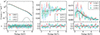 |
Fig. 1. Energy distributions of the Stokes parameters I, Q, and U, along with the best-fit model (top), and the residuals between the data and the model normalized by the errors (bottom). |
Phase-averaged spectro-polarimetric results.
To test for a possible energy dependence of the polarization properties in Cen X-3, we replaced the polconst component in the best-fit model with pollin. Applying this modified model to the phase-averaged data resulted in a modest improvement in fit quality, giving χ2/d.o.f. = 583.4/606, a PA slope of −3.9 ± 1.2 deg keV−1, and a PD slope of −0.3 ± 0.2% keV−1, as listed in Table 2. An F-test yielded a p-value of 0.0017, indicating a potential energy dependence of the polarization. The slope of the PD is close to zero, indicating that the PD is approximately constant with energy. Accordingly, we fixed the PD slope at zero, which resulted in a PA value and PA slope identical to those obtained when the PD slope was allowed to vary. We further evaluated this using maximum likelihood estimation (MLE) for both constant and linear PA models. The Bayesian information criterion (BIC) values for the constant and linear models were 11.46 and 6.51, respectively, suggesting that the linear model is preferred. This preference for a linear energy dependence of the PA is consistent with the findings of Tsygankov et al. (2022).
We performed an energy-resolved analysis using pcube, dividing the 2–8 keV range into six 1-keV-wide sub-bands, with results shown in Fig. 2. We conducted a complementary energy-resolved spectro-polarimetric analysis within the individual sub-bands. Due to limited photon statistics in the narrow energy bins, spectral parameters in each sub-band were fixed to the best-fit values obtained for the full 2–8 keV range. The polconst model was used to estimate the PD and PA, with only these parameters allowed to vary. As shown in Fig. 2, the PD shows no significant energy dependence, while the PA exhibits only a marginal trend with energy.
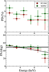 |
Fig. 2. Phase-averaged energy dependence of the PD and PA for Cen X-3. The solid black and dashed lines represent the constant and linear fits to the PA variation with energy, obtained using MLE. |
Given the strong phase dependence of polarization in XRPs, we further explored the dependence of polarization on both energy and pulse phase, dividing the pulse phase into seven equal bins. The 2–8 keV band was divided into three 2-keV-wide sub-bands, and the results are presented in Figs. 3 and 4. As shown in the top panel of Fig. 4, the normalized pulse profiles are largely consistent across energies, suggesting limited spectral evolution over phase in the narrow energy band of IXPE. In terms of polarization properties, we observe that the PA exhibits significant energy dependence in a few phase bins.
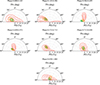 |
Fig. 3. Polarization vectors as a function of pulse phase for Cen X–3 in three energy bands: 2–4 keV (green), 4–6 keV (orange), and 6–8 keV (red). In each plot, the PD and PA contours are shown at the 68.27%, 95.45%, and 99.73% confidence levels. |
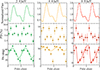 |
Fig. 4. Pulse phase-resolved, energy-dependent polarimetric results. Top panels: Normalized pulse profiles in three energy bands. Middle panels: Variations of PD with pulse phase. Bottom panels: Variations of PA with pulse phase. The 2–4, 4–6, and 6–8 keV bands are shown in the left, middle, and right columns and are color-coded in green, orange, and red, respectively. The solid curves in the bottom panels represent the best-fitting single-component RVM models applied to the PA data. |
We used the RVM to model the phase-resolved PA modulation. This model has been widely used to infer the geometrical parameters of accreting XRPs from phase-resolved polarimetric data (e.g., Doroshenko et al. 2022; Tsygankov et al. 2022; Mushtukov et al. 2023; Marshall et al. 2022; Heyl et al. 2024; Forsblom et al. 2024, 2025; Poutanen et al. 2024; Zhao et al. 2024, 2025). The RVM describes PA variation as a function of pulse phase under the assumption that radiation predominantly escapes in the O-mode. The PA predicted by the RVM is given by Poutanen (2020)
 (1)
(1)
where ip is the inclination angle between the observer’s line of sight and the pulsar’s spin axis, θ is the magnetic obliquity, χp is the position angle of the spin axis on the sky, and ϕ0 is the pulse phase at which the magnetic axis is closest to the observer.
To account for the non-Gaussian nature of the PA, we adopted the likelihood formalism introduced by Naghizadeh-Khouei & Clarke (1993), which is based on the probability distribution of the measured PA (denoted ψ). The corresponding probability density function G(ψ) is defined as
![Mathematical equation: $$ \begin{aligned} G(\psi ) = \frac{1}{\sqrt{\pi }} \left\{ \frac{1}{\sqrt{\pi }} + \eta \,\mathrm{e} ^{\eta ^2} \left[1 + \mathrm{erf} (\eta )\right] \right\} \mathrm{e} ^{-p_0^2/2}, \end{aligned} $$](/articles/aa/full_html/2026/04/aa56184-25/aa56184-25-eq10.gif) (2)
(2)
where  is the signal-to-noise ratio of the PD,
 ![Mathematical equation: $ \eta = p_0 \cos [2(\chi - \chi _0)]/\sqrt{2} $](/articles/aa/full_html/2026/04/aa56184-25/aa56184-25-eq12.gif) , and
, and  is the measured PA derived from the Stokes parameters. Here, χ denotes the model-predicted PA, and erf is the standard error function. We performed parameter inference in each energy band using the affine-invariant Markov chain Monte Carlo (MCMC) sampler emcee (Foreman-Mackey et al. 2013). The best-fit parameters derived using the RVM are summarized in Table 3 with the best-fit models shown in the lower panel of Fig. 4 and the posterior distributions shown in Fig. 5. The position angle of the spin axis (χp) and the magnetic obliquity (θ) are broadly consistent across different energy bands. The most notable variations are observed in ip and ϕ0, which show a clear energy dependence. The RVM parameters obtained from the 2–4 keV band closely match those reported by Tsygankov et al. (2022), which is not surprising since the low-energy photons tend to dominate when multiple energy bands are combined.
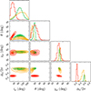 |
Fig. 5. Corner plots of the posterior distributions of the the single-component RVM parameters for the 2–4 keV (green), 4–6 keV (orange), and 6–8 keV (red) ranges. |
Single-RVM best-fit parameters for the three energy bands.
Such variation in RVM parameters across energy bands is generally not expected under standard RVM assumptions. Recent studies of XRPs, notably RX J0440.9+4431 (Doroshenko et al. 2023; Zhao et al. 2025) and Swift J0243.6+6124 (Poutanen et al. 2024), have reconciled similar discrepancies where RVM parameters appeared to vary significantly over time. This was achieved by introducing an additional phase-independent polarized component. In this two-component model, the observed emission is modeled as a combination of a pulsed, phase-dependent component and an additional unpulsed, phase-independent one. Under this framework, the PA variations can be reproduced using a single set of RVM parameters. The total Stokes parameters can be expressed as the sum of contributions from both components:
 (3)
(3)
where the subscripts “p” and “a” denote the pulsed and additional polarized components, respectively. The Stokes parameters are normalized to the average flux. The Q and U parameters are further related to the PD, PA, and polarized flux (PF) through the following expressions:
![Mathematical equation: $$ \begin{aligned} Q_{\mathrm{p} }(\phi )&= \mathrm{PD} _{\mathrm{p} }(\phi ) \, I_{\mathrm{p} }(\phi ) \cos [2\chi (\phi )] = \mathrm{PF} _{\mathrm{p} }(\phi ) \cos [2\chi (\phi )], \nonumber \\ U_{\mathrm{p} }(\phi )&= \mathrm{PD} _{\mathrm{p} }(\phi ) \, I_{\mathrm{p} }(\phi ) \sin [2\chi (\phi )] = \mathrm{PF} _{\mathrm{p} }(\phi ) \sin [2\chi (\phi )], \\ Q_{\mathrm{a} }&= \mathrm{PD} _{\mathrm{a} } \, I_{\mathrm{a} } \cos (2\chi _{\mathrm{a} }) = \mathrm{PF} _{\mathrm{a} } \cos (2\chi _{\mathrm{a} }), \nonumber \\ U_{\mathrm{a} }&= \mathrm{PD} _{\mathrm{a} } \, I_{\mathrm{a} } \sin (2\chi _{\mathrm{a} }) = \mathrm{PF} _{\mathrm{a} } \sin (2\chi _{\mathrm{a} }). \nonumber \end{aligned} $$](/articles/aa/full_html/2026/04/aa56184-25/aa56184-25-eq23.gif) (4)
(4)
Here, PDp(ϕ) and PDa represent the PDs of the pulsed and additional components, respectively; χ(ϕ) is the PA of the pulsed component; and χa denotes the PA of the additional component.
We fitted the observed phase-resolved Stokes parameters I, Q, and U, assuming uniform priors for most parameters. For the inclination angle ip and magnetic obliquity θ, flat priors were assumed for cos ip and cosθ. The likelihood function was constructed using χ2 statistics for Q and U following Doroshenko et al. (2023). The parameter ranges were set as follows: ip ∈ [0° ,180° ], θ ∈ [0° ,90° ], χp ∈ [ − 90° ,90° ], ϕp/(2π)∈[0, 1], PDa ∈ [0, 0.3], PDp ∈ [0, 1], and Ia ≤ min[I(ϕ)]. The MCMC fitting yields posterior distributions for the RVM geometrical parameters and the unpulsed Stokes components (Ia, Qa, and Ua). From these unpulsed components, we derived the distributions of the polarization flux and angle for the constant component (PFc and χc), which are displayed in Fig. A.1. To determine the phase-resolved properties of the pulsed component, we subtracted the unpulsed contribution from the observed Stokes parameters for each sample in the chain. This allowed us to derive the posterior distributions for the pulsed PA (PAp), as shown in Figs. A.2–A.4. Figure 6 shows the phase-resolved PAs of the pulsed components in three energy bands, overlaid with the best-fit RVM curves. The dashed lines indicate the inferred PA of the unpulsed component, which remains roughly the same across the different energy bands. However, even with the inclusion of this additional component, significant deviations from the RVM predictions persist in a few phase bins.
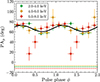 |
Fig. 6. PA for the pulsed components of Cen X-3 in different energy bands, as indicated by the colored points. The constant components are shown as dashed lines. The solid black line represents the joint RVM fit for the three energy bands after subtraction of the constant components. The color coding is the same as in Fig. 4. |
Notably, the energy dependence of PA is strongly phase-dependent, as illustrated in Fig. 4. In most phase bins, the PAs are consistent across energy bands. However, in the phase intervals 0.286–0.429 and 0.429–0.572, the PA exhibits a clear energy dependence. To further illustrate this difference, we plot two phase intervals: 0.143–0.286 and 0.286–0.429. As shown in Fig. 7, these two intervals display qualitatively different PA evolution with energy: one shows a clear linear trend, while the other remains nearly constant. This suggests that the contribution of the additional component may be phase-dependent. It is interesting to note that the phase intervals 0.286–0.429 and 0.429–0.572 correspond to the main peak of the pulse profile.
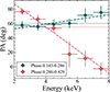 |
Fig. 7. Energy dependence of the PA for the phase intervals 0.143–0.286 and 0.286–0.429. The solid and dashed lines represent the constant and linear fits, respectively. BIC values (constant/linear) are 6.96/5.01 for phase 0.143–0.286 and 93.35/6.06 for phase 0.286–0.429. |
The additional component is thought to originate from scattering in the disk wind or magnetospheric accretion flow. In such scenarios, the flux of scattered X-ray photons varies with pulse phase, resulting in an enhanced scattering contribution at specific viewing angles. Consequently, the Stokes parameters of this additional component exhibit phase-dependent variations. To account for this possibility, we can revise Eq. (3) by allowing the Stokes parameters of the additional component to vary with phase:
 (5)
(5)
The PA of the additional component depends on several factors, including the opening angle of the disk wind and the angular distribution of the incident photons (Nitindala et al. 2025). For simplicity, we assumed that the PA is constant and expressed as
 (6)
(6)
Here we assume that only the PF of the additional component varies with phase, while its PA χa remains fixed. Hence, we treated χa as a global free parameter across all pulse phases and allowed Qa(ϕ) to vary independently in each phase bin. The corresponding Stokes U parameter was then computed as
 (7)
(7)
In our analysis, we assumed that the RVM parameters of the pulsed component are independent of energy. To mitigate the degeneracy between the pulsed and additional components and to reduce the number of free parameters, we fixed the RVM geometry to the best-fit values obtained from the 2.0–4.0 keV band (see values in Table 3). This choice is motivated by the fact that ip from the 2.0–4.0 keV band are more consistent with the orbital inclination (Ash et al. 1999) and the magnetic obliquity θ agrees well with results from pulse profile modeling (Kraus et al. 1996). For each energy band, we fitted eight free parameters: seven parameters of Qa(ϕ) corresponding to different pulse phase bins, and one parameter for the PA χa of the additional component. Across the three energy bands analyzed, the total number of free parameters amounts to 24. The fitting results are presented in Fig. 8, and the posterior distributions are plotted in Figs. A.5–A.7. The bottom panel of Fig. 8 illustrates that the PA variations with pulse phase across the different energy bands are well reproduced by a single set of RVM parameters, supporting the assumption of energy-independent geometry. The inferred PA of the additional component, χa, remains approximately consistent across energy bands. In this fitting, we assumed that the PA of the additional component is constant with phase, while its PF was allowed to vary with pulse phase.
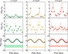 |
Fig. 8. Pulse phase-resolved polarization properties decomposed into pulsed and additional components for each energy band. Top: PDs (in total flux) of the additional component (PDa). Middle: PDs of the pulsed component (PDp). When the PDs are detected with a confidence level below 68% (1σ), the corresponding 1σ upper limits are shown as downward arrows in darker colors. Bottom: PA of the pulsed component (PAp) versus pulse phase. The shaded horizontal bands indicate the phase-independent PAs of the additional component, while the solid black curves represent the best-fit RVM to the pulsed component. |
3.2. Spectral analysis
To further investigate the origin of the observed energy dependence in the PA, we performed a broadband spectral analysis using IXPE, NICER, and NuSTAR observations. Since no simultaneous NICER and NuSTAR observations were available during the IXPE coverage, we selected archival observations corresponding to the same high state. The luminosities during the IXPE, NICER, and NuSTAR observations are comparable, being approximately (2.3–2.4)×1037 erg s−1 in the 2–8 keV energy band. In Fig. 9, we present the pulse profiles obtained with IXPE, NICER, and NuSTAR in the 4–8 keV band. The IXPE pulse profile shows slight differences compared to the NICER pulse profile. Since the observations are not simultaneous, such differences may reflect intrinsic temporal variability of the source, potentially including precessional effects of the neutron star. Furthermore, the pulse fraction measured by NuSTAR is significantly lower than that obtained from the simultaneous NICER observation. This discrepancy may be attributable to dead-time effects in NuSTAR and warrants further investigation, which is beyond the scope of this paper.
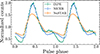 |
Fig. 9. Normalized pulse profiles of IXPE (blue), NICER (green), and NuSTAR (orange) in the same energy band (4–8 keV). |
For the spectra analysis, we adopted a commonly used phenomenological model for XRPs: highecut*powerlaw, where the highecut component is known for its sharp spectral drop at the cutoff energy, as widely discussed in previous studies (Kretschmar et al. 1997; Kreykenbohm et al. 1999; Coburn et al. 2002). To account for this sharp dip, we included a multiplicative gabs component. The centroid line energy is linked to the cutoff energy. Another gabs was included to account for the absorption structure around 2.2 keV in the NICER spectrum, which is likely associated with the gold M-shell absorption edge. A Gaussian component was added to model the iron fluorescence line, and an additional Gaussian was introduced to address known calibration issues around ∼1 keV for NICER. The interstellar absorption was modeled using tbabs, while for intrinsic absorption, we also included the pcfabs component.
As shown in the bottom panel of Fig. 10, the spectrum exhibits a clear cyclotron resonance scattering feature (CRSF) around 30 keV, which we modeled with an additional gabs component. To correct for cross-calibration offsets between instruments, we applied the constant model. Thus, our final spectral model is constant*tbabs*pcfabs*(highecut*powerlaw*gabs*gabs + gauss + gauss)*gabs.
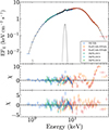 |
Fig. 10. Broadband spectral energy distribution of Cen X-3 with IXPE, NICER, and NuSTAR. Top panel: Unfolded spectrum with the best-fit model (solid line). Middle panel: Residuals showing a prominent absorption feature at ∼30 keV consistent with a CRSF. Bottom panel: Residuals after including the CRSF component. The best-fit model is constant*tbabs*pcfabs*(highecut*powerlaw*gabs*gabs + gauss + gauss)*gabs. |
This model provides a satisfactory fit to the broadband spectrum over the 0.7–79 keV range. In this fit, We let the instrument gains of NICER and IXPE vary as free parameters. The best-fit parameter values are listed in Table 4. The hydrogen column density is NH ≈ 1.256 × 1022 cm−2, which is close to the 1.1 × 1022 cm−2 value inferred from the HI4PI survey map (HI4PI Collaboration 2016)3.
Best-fit parameters for the phase-averaged joint spectra of IXPE, NICER, and NuSTAR.
We then performed a phase-resolved spectral analysis using the same model described above. For the pulse phase intervals where the CRSF was not statistically significant, we omitted the additional gabs component. For the phase-resolved fits, we fixed the column density of tbabs to the phase-averaged best-fit value, NH = 1.256 × 1022 cm−2, since interstellar absorption is not expected to vary with pulse phase. The best-fit parameters for the phase-resolved spectral analysis are listed in Table 5 and are shown in Fig. 11. The parameters exhibit strong phase-dependent variability, as expected given the highly anisotropic emission region geometry of XRPs.
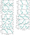 |
Fig. 11. Variations in spectral parameters with pulse phase. The left axes exhibit the spectral parameter evolution with pulse phase, while the right axes show the pulse profiles of NuSTAR in the 4–79 keV range. The parameters shown are: NH – hydrogen column density from the pcfabs component (×1022 cm−2), representing intrinsic absorption; covering fraction – fraction of the source covered by absorbing material; Ecut – cutoff energy in the highecut component (keV); Efold – e-folding energy in the highecut component (keV); Γ – photon index of the power-law component; PD – polarization degree; PA – polarization angle; Ecyc – CRSF centroid energy (keV); σcyc – width of the CRSF line (keV); line depth – optical depth of the CRSF; Egauss – centroid energy of the iron fluorescence line (keV); EWgauss – equivalent width of the iron line (keV); Normgauss – normalization of the iron line component. |
Best-fit parameters for the phase-resolved IXPE (2–8 keV), NICER (0.7–10 keV), and NuSTAR (4–79 keV) spectra.
Although most spectral parameters exhibit complex evolution with pulse phase, the photon index Γ shows an anticorrelation with flux, while the CRSF line energy displays a clear positive correlation. Of particular interest are the hydrogen column density (NH) and the covering fraction from the pcfabs component, which we interpret as tracers of intervening wind material. Both parameters exhibit significant modulation with pulse phase, suggesting that the properties of the wind may also vary during the pulsation cycle.
4. Discussion and summary
IXPE observations have revealed both new insights and challenges in understanding XRPs. The observed low PDs, which fall significantly below theoretical predictions, warrant a reexamination of current models, particularly with respect to potential depolarization mechanisms. Further theoretical work will help elucidate the underlying mechanisms responsible for the observed PDs and their energy dependence. Despite this, the variations in PA with pulse phase in most XRPs continue to be well described by the RVM, consistent with the predictions of vacuum birefringence. In this framework, the observed PA tracks the direction of the local magnetic field, enabling the determination of XRP geometric parameters. Since PA is expected to follow magnetic field geometry, it should show little to no dependence on photon energy for the radiation within the adiabatic radius.
Tsygankov et al. (2022) performed a detailed polarimetric study of Cen X-3, including phase-averaged, phase-resolved, and phase-averaged energy-resolved analyses. In the present work, we extended this investigation by examining the phase-resolved energy dependence of the polarization. By dividing the data into three equal energy bands, we performed a phase-resolved analysis within each band. Our results show that, while the phase-averaged PA exhibits only a weak dependence on energy, a few phase bins display a pronounced PA energy dependence. Moreover, the pattern of PA variation with energy differs across the phase bins, as illustrated in Fig. 7. This strong, phase-dependent energy behavior of the PA is inconsistent with the predictions of vacuum birefringence.
However, mode conversion between the O- and X- modes at the vacuum resonance can introduce a 90° shift in PA. IXPE observations of Vela X-1 (Forsblom et al. 2025) revealed exactly such a 90° PA swing between the low- and high-energy bands in the phase-averaged data. A phase-resolved analysis detected significant polarization in only one phase interval at low energy; a comparison with the corresponding high-energy interval again showed a 90° offset. The observed signatures for this source are naturally explained by vacuum-resonance–driven mode conversion. In Cen X-3, however, the PA evolution with energy departs from the exact 90° flip predicted for vacuum-resonance mode conversion. Instead, the PA in the 0.286–0.429 phase range shows a distinct linear trend with energy (Fig. 7), indicating that this mechanism alone cannot account for the observed behavior. A phase-averaged investigation by Loktev et al. (2025) uncovered a ∼70° PA shift between the low- and high-energy bands for 4U 1538−52. Moreover, phase-resolved data present an even more intricate picture: pulse-phase–dependent PA offsets diverge from the 90° prediction, indicating that vacuum-resonance mode conversion cannot by itself explain the observed polarimetric behavior of this source.
Although the energy dependence of polarization remains insufficiently explored in many XRPs, some sources already exhibit pronounced epoch-to-epoch variations in their PA profiles as a function of pulse phase–for example, RX J0440.9+4431/LS V +44 17 (Doroshenko et al. 2023; Zhao et al. 2025) and Swift J0243.6+6124 (Poutanen et al. 2024). In both cases, the PA varies markedly between observations. Introducing an additional, non-pulsating polarized component allows these disparate PA patterns to be reconciled with a single set of RVM parameters. This non-pulsating polarized component could plausibly arise from scattering in the disk wind or within the magnetospheric accretion flow. Fig. 6 shows the two-component RVM fit, which assumes a phase-independent PF and PA for the additional component. Although introducing the constant polarized component, a few data points still deviate from the model curve, indicating that even this framework does not fully capture the observed behavior. As shown in Figs. 3 and 4, the strongest energy dependence of the PA occurs in the phase interval 0.286–0.572, corresponding to the peak of the pulse profile. This indicates that the polarization properties of this additional component may also vary with phase. We therefore relaxed the assumption of constant PF and allowed it to vary with pulse phase by considering that the observed polarized signal depends on the phase-dependent illuminating flux. In addition, variations in the disk wind properties may also lead to changes in the additional scattered component across pulse phase (Nitindala et al. 2025). This naturally leads to the expectation that the additional scattering-induced PF should modulate with phase. As shown in Fig. 8, allowing the PF to vary enables the PA of the pulsating component to be well reproduced using a single set of RVM parameters. In this fit, since the PF is no longer fixed across phases, the four RVM parameters do not converge to meaningful values when left free. We therefore fixed them to the best-fit values obtained from the 2–4 keV band. As evident from the fit, the PF of the additional component varies with pulse phase. The PA of this component across different energy bands is broadly consistent. As discussed in Doroshenko et al. (2023), this additional component may originate from scattering in the disk wind. Since the wind is located well beyond the adiabatic radius, the vacuum birefringence predictions can still hold true when this contribution is taken into account. If the additional component originates from scattering in the disk wind, its PA can naturally be associated with the disk axis, while optical polarization from scattering in the disk may provide an independent measure of the disk orientation. Therefore, optical polarization measurements would offer a valuable way to evaluate this interpretation.
We also performed a broadband spectral analysis using IXPE, NICER, and NuSTAR data. In this analysis, we employed the pcfabs model to trace the properties of the disk wind. A phase-resolved spectral analysis reveals that both the column density (NH) and covering fraction inferred from pcfabs exhibit significant modulation with pulse phase, as shown in Fig. 11. The variation in covering fraction suggests that the scattered flux also varies with pulse phase rather than remaining constant. In addition, a reflected Fe line is clearly present in the spectra and exhibits pronounced variations with pulse phase. These spectral results indicate that the disk wind properties vary with pulse phase, providing a natural explanation for the observed phase-dependent variations in the PF of the additional component.
However, it should be noted that the polarization properties of the additional component depend on several factors, including the geometry of the scattering region and the beaming pattern of the pulsar emission. The response of the scattered component to the illuminating flux should be examined in greater detail – for example, through dedicated Monte Carlo simulations. In this work, due to limited photon statistics and for simplicity, we allowed only the PF of the additional component to vary freely. We note that the PF of this component can reach up to approximately 6% (normalized by the total flux). Assuming an inclination of i = 70° and adopting the analytical expression PD = sin2i/(3 − cos2i) (Sunyaev & Titarchuk 1985), the expected PD of the scattered component is about 30% (self-normalized), and it is a weak function of inclination and the wind opening angle (Nitindala et al. 2025). This implies that the scattered component would contribute nearly 20% of the total flux, which is a considerable fraction. Further refinements to this picture may emerge as we better understand the scattered component’s actual flux contribution and polarization properties. The observed energy-dependent polarization behavior provides a useful context for developing theoretical models that incorporate more complex scattering geometries or additional polarization mechanisms. In addition, future missions such as the enhanced X-ray Timing and Polarimetry mission (eXTP, Zhang et al. 2025; Ge et al. 2025) will offer greatly improved polarimetric statistics, enabling more robust tests of these scenarios.
Acknowledgments
We thank the anonymous referee for the constructive comments that helped improve the manuscript. Financial support for this work is provided by the National Key R&D Program of China (2021YFA0718500). We also acknowledge funding from the National Natural Science Foundation of China (NSFC) under grant numbers 12122306, 12333007, and U2038102. We acknowledge support from the China’s Space Origins Exploration Program. This research was supported by the International Space Science Institute (ISSI) in Bern, through International Team project 25-657 ‘Polarimetric Insights into Extreme Magnetism’. SST and JP acknowledge support by the Research Council of Finland, the Centre of Excellence in Neutron-Star Physics (project 374064).
References
- Arnason, R. M., Papei, H., Barmby, P., Bahramian, A., & Gorski, M. D. 2021, MNRAS, 502, 5455 [NASA ADS] [CrossRef] [Google Scholar]
- Arnaud, K. A. 1996, ASP Conf. Ser., 101, 17 [Google Scholar]
- Ash, T. D. C., Reynolds, A. P., Roche, P., et al. 1999, MNRAS, 307, 357 [NASA ADS] [CrossRef] [Google Scholar]
- Baldini, L., Bucciantini, N., Di Lalla, N., et al. 2022, SoftwareX, 19, 101194 [NASA ADS] [CrossRef] [Google Scholar]
- Basko, M. M., & Sunyaev, R. A. 1976, MNRAS, 175, 395 [Google Scholar]
- Caiazzo, I., & Heyl, J. 2021, MNRAS, 501, 129 [Google Scholar]
- Coburn, W., Heindl, W. A., Rothschild, R. E., et al. 2002, ApJ, 580, 394 [NASA ADS] [CrossRef] [Google Scholar]
- Di Marco, A., Costa, E., Muleri, F., et al. 2022, AJ, 163, 170 [NASA ADS] [CrossRef] [Google Scholar]
- Di Marco, A., Soffitta, P., Costa, E., et al. 2023, AJ, 165, 143 [CrossRef] [Google Scholar]
- Doroshenko, V., Poutanen, J., Tsygankov, S. S., et al. 2022, Nat. Astron., 6, 1433 [NASA ADS] [CrossRef] [Google Scholar]
- Doroshenko, V., Poutanen, J., Heyl, J., et al. 2023, A&A, 677, A57 [NASA ADS] [CrossRef] [EDP Sciences] [Google Scholar]
- Feng, H., Jiang, W., Minuti, M., et al. 2019, Exp. Astron., 47, 225 [NASA ADS] [CrossRef] [Google Scholar]
- Foreman-Mackey, D., Hogg, D. W., Lang, D., & Goodman, J. 2013, PASP, 125, 306 [Google Scholar]
- Forsblom, S. V., Poutanen, J., Tsygankov, S. S., et al. 2023, ApJ, 947, L20 [NASA ADS] [CrossRef] [Google Scholar]
- Forsblom, S. V., Tsygankov, S. S., Poutanen, J., et al. 2024, A&A, 691, A216 [NASA ADS] [CrossRef] [EDP Sciences] [Google Scholar]
- Forsblom, S. V., Tsygankov, S. S., Suleimanov, V. F., Mushtukov, A. A., & Poutanen, J. 2025, A&A, 696, A224 [NASA ADS] [CrossRef] [EDP Sciences] [Google Scholar]
- Garg, A., Rawat, D., Bhargava, Y., Méndez, M., & Bhattacharyya, S. 2023, ApJ, 948, L10 [NASA ADS] [CrossRef] [Google Scholar]
- Ge, M., Ji, L., Taverna, R., et al. 2025, Sci. China: Phys. Mech. Astron., 68, 119505 [Google Scholar]
- Gendreau, K. C., Arzoumanian, Z., Adkins, P. W., et al. 2016, Proc. SPIE, 9905, 99051H [NASA ADS] [CrossRef] [Google Scholar]
- Giacconi, R., Gursky, H., Kellogg, E., Schreier, E., & Tananbaum, H. 1971, ApJ, 167, L67 [NASA ADS] [CrossRef] [Google Scholar]
- Gnedin, Y. N., Pavlov, G. G., & Shibanov, Y. A. 1978, Soviet. Astron. Lett., 4, 117 [Google Scholar]
- Harrison, F. A., Craig, W. W., Christensen, F. E., et al. 2013, ApJ, 770, 103 [Google Scholar]
- Heyl, J., & Caiazzo, I. 2018, Galaxies, 6, 76 [NASA ADS] [CrossRef] [Google Scholar]
- Heyl, J. S., & Shaviv, N. J. 2000, MNRAS, 311, 555 [NASA ADS] [CrossRef] [Google Scholar]
- Heyl, J. S., & Shaviv, N. J. 2002, Phys. Rev. D, 66, 023002 [NASA ADS] [CrossRef] [Google Scholar]
- Heyl, J., Doroshenko, V., González-Caniulef, D., et al. 2024, Nat. Astron., 8, 1047 [NASA ADS] [CrossRef] [Google Scholar]
- HI4PI Collaboration (Ben Bekhti, N., et al.) 2016, A&A, 594, A116 [NASA ADS] [CrossRef] [EDP Sciences] [Google Scholar]
- Kislat, F., Clark, B., Beilicke, M., & Krawczynski, H. 2015, Astropart. Phys., 68, 45 [NASA ADS] [CrossRef] [Google Scholar]
- Kraus, U., Blum, S., Schulte, J., Ruder, H., & Meszaros, P. 1996, ApJ, 467, 794 [NASA ADS] [CrossRef] [Google Scholar]
- Kretschmar, P., Kreykenbohm, I., Wilms, J., et al. 1997, ESA SP, 382, 141 [Google Scholar]
- Kreykenbohm, I., Kretschmar, P., Wilms, J., et al. 1999, A&A, 341, 141 [NASA ADS] [Google Scholar]
- Krzeminski, W. 1974, ApJ, 192, L135 [NASA ADS] [CrossRef] [Google Scholar]
- Loktev, V., Forsblom, S. V., Tsygankov, S. S., et al. 2025, A&A, 698, A22 [NASA ADS] [CrossRef] [EDP Sciences] [Google Scholar]
- Long, X., Feng, H., Li, H., et al. 2023, ApJ, 950, 76 [NASA ADS] [CrossRef] [Google Scholar]
- Majumder, S., Chatterjee, R., Jayasurya, K. M., Das, S., & Nandi, A. 2024, ApJ, 971, L21 [NASA ADS] [CrossRef] [Google Scholar]
- Malacaria, C., Heyl, J., Doroshenko, V., et al. 2023, A&A, 675, A29 [NASA ADS] [CrossRef] [EDP Sciences] [Google Scholar]
- Marshall, H. L., Ng, M., Rogantini, D., et al. 2022, ApJ, 940, 70 [NASA ADS] [CrossRef] [Google Scholar]
- Meszaros, P., Novick, R., Szentgyorgyi, A., Chanan, G. A., & Weisskopf, M. C. 1988, ApJ, 324, 1056 [NASA ADS] [CrossRef] [Google Scholar]
- Mushtukov, A., & Tsygankov, S. 2024, in Handbook of X-ray and Gamma-ray Astrophysics, eds. C. Bambi, & A. Santangelo (Singapore: Springer), 4105 [Google Scholar]
- Mushtukov, A. A., Tsygankov, S. S., Poutanen, J., et al. 2023, MNRAS, 524, 2004 [NASA ADS] [CrossRef] [Google Scholar]
- Naghizadeh-Khouei, J., & Clarke, D. 1993, A&A, 274, 968 [NASA ADS] [Google Scholar]
- Nitindala, A. P., Veledina, A., & Poutanen, J. 2025, A&A, 694, A230 [NASA ADS] [CrossRef] [EDP Sciences] [Google Scholar]
- Pavlov, G. G., & Shibanov, Y. A. 1979, Soviet. J. Exp. Theor. Phys., 49, 741 [Google Scholar]
- Poutanen, J. 2020, A&A, 641, A166 [NASA ADS] [CrossRef] [EDP Sciences] [Google Scholar]
- Poutanen, J., Tsygankov, S. S., Doroshenko, V., et al. 2024, A&A, 691, A123 [NASA ADS] [CrossRef] [EDP Sciences] [Google Scholar]
- Radhakrishnan, V., & Cooke, D. J. 1969, Astrophys. Lett., 3, 225 [NASA ADS] [Google Scholar]
- Raichur, H., & Paul, B. 2010, MNRAS, 401, 1532 [NASA ADS] [CrossRef] [Google Scholar]
- Soffitta, P., Baldini, L., Bellazzini, R., et al. 2021, AJ, 162, 208 [CrossRef] [Google Scholar]
- Suleimanov, V. F., Forsblom, S. V., Tsygankov, S. S., et al. 2023, A&A, 678, A119 [NASA ADS] [CrossRef] [EDP Sciences] [Google Scholar]
- Sunyaev, R. A., & Titarchuk, L. G. 1985, A&A, 143, 374 [NASA ADS] [Google Scholar]
- Taverna, R., & Turolla, R. 2024, Galaxies, 12, 6 [NASA ADS] [CrossRef] [Google Scholar]
- Taverna, R., Turolla, R., Gonzalez Caniulef, D., et al. 2015, MNRAS, 454, 3254 [NASA ADS] [CrossRef] [Google Scholar]
- Tsygankov, S. S., Doroshenko, V., Poutanen, J., et al. 2022, ApJ, 941, L14 [NASA ADS] [CrossRef] [Google Scholar]
- Tsygankov, S. S., Doroshenko, V., Mushtukov, A. A., et al. 2023, A&A, 675, A48 [NASA ADS] [CrossRef] [EDP Sciences] [Google Scholar]
- Weisskopf, M. C., Soffitta, P., Baldini, L., et al. 2022, JATIS, 8, 026002 [NASA ADS] [Google Scholar]
- Zhang, S.-N., Santangelo, A., Xu, Y., et al. 2025, Sci. China: Phys. Mech. Astron., 68, 119502 [Google Scholar]
- Zhao, Q. C., Li, H. C., Tao, L., et al. 2024, MNRAS, 531, 3935 [NASA ADS] [CrossRef] [Google Scholar]
- Zhao, Q. C., Tao, L., Tsygankov, S. S., et al. 2025, A&A, 693, A241 [NASA ADS] [CrossRef] [EDP Sciences] [Google Scholar]
Appendix A: Posterior distributions of two-component RVM
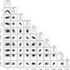 |
Fig. A.1. Corner plots of the posterior distributions for the two-component RVM model with phase-independent additional component. PFc i, i = 1, 2, 3 are the PF of the phase-independent additional component in unit of averaged flux for three energy bands (2–4, 4–6, and 6–8 keV). χc i are its PA. |
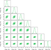 |
Fig. A.2. Corner plots of the posterior distributions for PA of pulsed component in 2–4 keV energy band. The parameters PApi (i = 1–7) represent the PA of the pulsed component in each of the seven phase bins. |
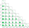 |
Fig. A.5. Corner plots of the posterior distributions for the two-component RVM model with phase-variable additional component for 2–4 keV band. The parameters PDi (i = 1–7) represent the PF fraction of the scattered component normalized by the total flux in each of the seven phase bins. χa denotes the constant PA of the scattered component. |
All Tables
Best-fit parameters for the phase-averaged joint spectra of IXPE, NICER, and NuSTAR.
Best-fit parameters for the phase-resolved IXPE (2–8 keV), NICER (0.7–10 keV), and NuSTAR (4–79 keV) spectra.
All Figures
|
Fig. 1. Energy distributions of the Stokes parameters I, Q, and U, along with the best-fit model (top), and the residuals between the data and the model normalized by the errors (bottom). |
| In the text | |
|
Fig. 2. Phase-averaged energy dependence of the PD and PA for Cen X-3. The solid black and dashed lines represent the constant and linear fits to the PA variation with energy, obtained using MLE. |
| In the text | |
|
Fig. 3. Polarization vectors as a function of pulse phase for Cen X–3 in three energy bands: 2–4 keV (green), 4–6 keV (orange), and 6–8 keV (red). In each plot, the PD and PA contours are shown at the 68.27%, 95.45%, and 99.73% confidence levels. |
| In the text | |
|
Fig. 4. Pulse phase-resolved, energy-dependent polarimetric results. Top panels: Normalized pulse profiles in three energy bands. Middle panels: Variations of PD with pulse phase. Bottom panels: Variations of PA with pulse phase. The 2–4, 4–6, and 6–8 keV bands are shown in the left, middle, and right columns and are color-coded in green, orange, and red, respectively. The solid curves in the bottom panels represent the best-fitting single-component RVM models applied to the PA data. |
| In the text | |
|
Fig. 5. Corner plots of the posterior distributions of the the single-component RVM parameters for the 2–4 keV (green), 4–6 keV (orange), and 6–8 keV (red) ranges. |
| In the text | |
|
Fig. 6. PA for the pulsed components of Cen X-3 in different energy bands, as indicated by the colored points. The constant components are shown as dashed lines. The solid black line represents the joint RVM fit for the three energy bands after subtraction of the constant components. The color coding is the same as in Fig. 4. |
| In the text | |
|
Fig. 7. Energy dependence of the PA for the phase intervals 0.143–0.286 and 0.286–0.429. The solid and dashed lines represent the constant and linear fits, respectively. BIC values (constant/linear) are 6.96/5.01 for phase 0.143–0.286 and 93.35/6.06 for phase 0.286–0.429. |
| In the text | |
|
Fig. 8. Pulse phase-resolved polarization properties decomposed into pulsed and additional components for each energy band. Top: PDs (in total flux) of the additional component (PDa). Middle: PDs of the pulsed component (PDp). When the PDs are detected with a confidence level below 68% (1σ), the corresponding 1σ upper limits are shown as downward arrows in darker colors. Bottom: PA of the pulsed component (PAp) versus pulse phase. The shaded horizontal bands indicate the phase-independent PAs of the additional component, while the solid black curves represent the best-fit RVM to the pulsed component. |
| In the text | |
|
Fig. 9. Normalized pulse profiles of IXPE (blue), NICER (green), and NuSTAR (orange) in the same energy band (4–8 keV). |
| In the text | |
|
Fig. 10. Broadband spectral energy distribution of Cen X-3 with IXPE, NICER, and NuSTAR. Top panel: Unfolded spectrum with the best-fit model (solid line). Middle panel: Residuals showing a prominent absorption feature at ∼30 keV consistent with a CRSF. Bottom panel: Residuals after including the CRSF component. The best-fit model is constant*tbabs*pcfabs*(highecut*powerlaw*gabs*gabs + gauss + gauss)*gabs. |
| In the text | |
|
Fig. 11. Variations in spectral parameters with pulse phase. The left axes exhibit the spectral parameter evolution with pulse phase, while the right axes show the pulse profiles of NuSTAR in the 4–79 keV range. The parameters shown are: NH – hydrogen column density from the pcfabs component (×1022 cm−2), representing intrinsic absorption; covering fraction – fraction of the source covered by absorbing material; Ecut – cutoff energy in the highecut component (keV); Efold – e-folding energy in the highecut component (keV); Γ – photon index of the power-law component; PD – polarization degree; PA – polarization angle; Ecyc – CRSF centroid energy (keV); σcyc – width of the CRSF line (keV); line depth – optical depth of the CRSF; Egauss – centroid energy of the iron fluorescence line (keV); EWgauss – equivalent width of the iron line (keV); Normgauss – normalization of the iron line component. |
| In the text | |
|
Fig. A.1. Corner plots of the posterior distributions for the two-component RVM model with phase-independent additional component. PFc i, i = 1, 2, 3 are the PF of the phase-independent additional component in unit of averaged flux for three energy bands (2–4, 4–6, and 6–8 keV). χc i are its PA. |
| In the text | |
|
Fig. A.2. Corner plots of the posterior distributions for PA of pulsed component in 2–4 keV energy band. The parameters PApi (i = 1–7) represent the PA of the pulsed component in each of the seven phase bins. |
| In the text | |
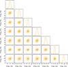 |
Fig. A.3. Same as Fig. A.2, but for 4–6 keV energy band. |
| In the text | |
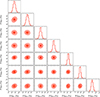 |
Fig. A.4. Same as Fig. A.2, but for 6–8 keV energy band. |
| In the text | |
|
Fig. A.5. Corner plots of the posterior distributions for the two-component RVM model with phase-variable additional component for 2–4 keV band. The parameters PDi (i = 1–7) represent the PF fraction of the scattered component normalized by the total flux in each of the seven phase bins. χa denotes the constant PA of the scattered component. |
| In the text | |
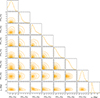 |
Fig. A.6. Same as Fig. A.5, but for 4–6 keV band. |
| In the text | |
 |
Fig. A.7. Same as Fig. A.5, but for 6–8 keV band. |
| In the text | |
Current usage metrics show cumulative count of Article Views (full-text article views including HTML views, PDF and ePub downloads, according to the available data) and Abstracts Views on Vision4Press platform.
Data correspond to usage on the plateform after 2015. The current usage metrics is available 48-96 hours after online publication and is updated daily on week days.
Initial download of the metrics may take a while.