| Issue |
A&A
Volume 708, April 2026
|
|
|---|---|---|
| Article Number | A37 | |
| Number of page(s) | 14 | |
| Section | Planets, planetary systems, and small bodies | |
| DOI | https://doi.org/10.1051/0004-6361/202557243 | |
| Published online | 27 March 2026 | |
The PAIRS project: a global formation model for planets in binaries
I. Effect of disc truncation on the growth of S-type planets
1
Department of Astronomy, University of Geneva,
Chemin Pegasi 51,
1290
Versoix,
Switzerland
2
Instituto de Astrofísica de La Plata, CCT La Plata-CONICET-UNLP, Paseo del Bosque S/N (1900),
La Plata,
Argentina
3
Department of Space Research & Planetary Sciences, University of Bern,
Gesellschaftsstrasse 6,
3012
Bern,
Switzerland
★ Corresponding author: This email address is being protected from spambots. You need JavaScript enabled to view it.
Received:
15
September
2025
Accepted:
9
January
2026
Abstract
Binary stars are as common as single stars. The number of detected planets orbiting binaries is rapidly increasing thanks to the synergy between transit surveys, Gaia, and high-resolution direct-imaging campaigns. However, global planet formation models around binary stars are still underdeveloped, which limits the theoretical understanding of planets orbiting binary star systems. We introduce the PAIRS project, which aims to build a global planet formation model for planets in binaries and to produce a planet population synthesis to statistically compare theory and observations. In this first paper, we present the adaptation of the circumstellar disc to simulate the formation of S-type planets. The presence of a secondary star tidally truncates and heats the outer part of the circumprimary disc (and vice versa for the circumsecondary disc), limiting the material to form planets. We implemented and quantified this effect for a range of binary parameters by adapting the Bern Model of planet formation in its pebble-based form and for in situ planet growth. We find that disc truncation has a strong impact on reducing the pebble supply for core growth and steadily suppresses planet formation for binary separations below 160 a when all the formed planets more massive than Mars are considered. Moreover, S-type planets tend to form close to the central star with respect to the binary separation and disc truncation radius. Our newly developed model will be the basis of future S-type planet population synthesis studies.
Key words: planets and satellites: formation / protoplanetary disks / binaries: general
© The Authors 2026
 Open Access article, published by EDP Sciences, under the terms of the Creative Commons Attribution License (https://creativecommons.org/licenses/by/4.0), which permits unrestricted use, distribution, and reproduction in any medium, provided the original work is properly cited.
This article is published in open access under the Subscribe to Open model. This email address is being protected from spambots. You need JavaScript enabled to view it. to support open access publication.
1 Introduction
Binary stars are very common. Half of the Sun-like stars in our Galaxy belong to a binary system (Raghavan et al. 2010). The detection of planets orbiting binary stars is rapidly increasing as the sensitivity and resolution of detectors improves. In the past few years, hundreds of planets that were first detected by transit surveys such as Kepler and the Transiting Exoplanet Survey Satellite (TESS) have been identified as belonging to a binary star system through astrometric follow-up by Gaia (e.g. Mugrauer & Michel 2021; Mugrauer et al. 2022; Behmard et al. 2022; Mugrauer et al. 2023) or high-resolution direct imaging (e.g. Lester et al. 2021; Sullivan et al. 2023; Schlagenhauf et al. 2024). These systems contain S-type planets, that is, planets orbiting one of the stars in the pair. The other type of planets in binaries is the circumbinary or P-type planet1. These are found around very close binaries, and in this case, the planet orbits both stars. P-type planets are very difficult to detect; we currently know about 30 of them (e.g. Doyle et al. 2011; Triaud et al. 2022; Martin 2018; Kostov et al. 2020, 2021; Socia et al. 2020; Standing et al. 2023). In contrast, about 500 S-type planets are either confirmed or validated today, and another 400 S-type planet candidates from TESS are awaiting confirmation (Mugrauer & Michel 2021; Mugrauer et al. 2022, 2023; Lester et al. 2021; Hirsch et al. 2021; Lester et al. 2022; Fontanive & Bardalez Gagliuffi 2021).
With already several hundred identified S-type planets, some statistics from observations have been inferred. For the occurrence rates, by combining direct imaging and radial velocities measurements, Hirsch et al. (2021) found that S-type giant planets with a semi-major axis between 0.1 and 20 au exist in 20% of binaries with separations larger than 100 au (a similar occurrence as for single stars), but in 4% of binaries with separations smaller than 100 au. This indicates a detrimental effect on giant planet formation for close binaries. By analysing Gaia Data Release 2, Fontanive & Bardalez Gagliuffi (2021) found that the distribution of planet mass and distance to the host star is statistically different for binaries and single stars as long as the two stars are closer than 1000 au. In addition, Lester et al. (2021) searched for companions to TESS systems known to host planets by direct imaging. They found that in contrast to field binaries, which have their peak of binary separation at 50 au, the most frequent binary separation is 100 au for planet-hosting binaries. The authors concluded that this indicates a detrimental effect of planet formation for binaries with separations closer than 100 au. They also found that planets in binaries span a wide size range, similar to exoplanets orbiting single stars. More recently, Thebault & Bonanni (2025) presented a new catalogue of planets in binaries. Of the different properties, they also analysed the distribution of binary separations for systems hosting planets and reporting a peak at 500 au. The study also highlighted based on recent surveys that about 20% of the known exoplanets are in reality S-type planets. Finally, Sullivan et al. (2023, 2024) analysed the properties of small S-type planet candidates from the Kepler survey for the first time in systems in which the secondary star was found by direct-imaging follow-up. In contrast to single-star planets, which exhibit a radius valley separating the population of super-Earths from the population of mini-Neptunes, the mini-Neptunes in S-type planets seem to be suppressed for binary separations smaller than 100 au (Sullivan et al. 2024).
In parallel, ALMA observations of discs around binaries in star-forming regions are starting to reveal the detrimental effect of a stellar companion on the dust mass, the extension of the dust disc, and the lifetime of S-type protoplanetary discs (Kutra et al. 2025; Zurlo et al. 2023, 2021, 2020; Barenfeld et al. 2019).
The rapidly growing population of S-type planets and discs and the first statistics of S-type planets call for the urgent development of planet formation models targeting the specific environment in which S-type planets form. This environment can indeed be very different from the single-star case. Namely, the presence of the stellar companion tidally truncates and heats the protoplanetary disc (Papaloizou & Pringle 1977; Artymowicz & Lubow 1994; Alexander et al. 2011), which reduces the reservoir of material for planet formation. In addition, the gravitational perturbation from the companion excites the orbits of the growing planets and planetesimals, which in principle precludes planetary accretion (Chambers et al. 2002). The closer the two stars, the more dramatic the effects (e.g Marzari & Thebault 2019).
The theoretical study of planet formation in binaries is still very limited to a few specific processes. The most explored processes are i) disc evolution (Alexander et al. 2011; Rosotti & Clarke 2018; Ronco et al. 2021; Zagaria et al. 2021), ii) planetesimal accretion (Marzari & Scholl 2000; Thébault et al. 2006; Silsbee & Rafikov 2015a,b; Rafikov & Silsbee 2015a,b), iii) dynamics after the dissipation of the gaseous disc (Thébault et al. 2004; Quintana & Lissauer 2006; Haghighipour 2006; Quintana et al. 2007; Giuppone et al. 2011), and iv) the study of the disc structure and planet migration via hydrodynamical simulations (Nelson 2003; Marzari et al. 2012; Kley & Nelson 2008; Kley & Haghighipour 2014; Kley et al. 2019; Jordan et al. 2021). However, some relevant physical processes operating in planet formation, such as pebble accretion (Ormel & Klahr 2010; Lambrechts & Johansen 2012, 2014), have never been included in the formation modelling of S-type planets so far. Pebble accretion has proven to be relevant to account for the short formation timescales of giant planets (e.g. Drążkowska et al. 2021) and to explain the properties of certain exoplanets (e.g. the dependence of the radius valley with the stellar mass, Venturini et al. 2024).
While it is essential to have reliable individual physical models, it is not enough to compare theory with observations of exoplanets. The individual physical processes operating during planet formation, such as core growth, gas accretion, disc evolution, and planet migration, all occur at similar timescales and feed back on each other. Because of this, they must be included in a single model when the simulation output is to be compared with observations. This is the principle of the so-called global or end-to-end planet formation models (e.g. Mordasini et al. 2015). This principle is also true for planet formation around binary stars.
Global planet formation models are a collection of 1D models and prescriptions that encapsulate the main processes acting during planet formation. The low dimensionality and simple nature of the individual models is essential to reduce computational time. When these global models are run thousands of times and the initial conditions stemming from observations are varied, the output is the so-called planet population synthesis (Ida & Lin 2004; Mordasini et al. 2009; Benz et al. 2014; Fortier et al. 2013; Ronco et al. 2017; Emsenhuber et al. 2021a). Global formation models and population synthesis for S-type planets are currently lacking. Without global formation models and population synthesis, a quantitative comparison between observations and theory for planets around binaries is not feasible.
We introduce here the PAIRS project. PAIRS stands for Planet formation Around bInary Stars. Its primary goal is to develop the first global planet formation model for S-type planets and to compute an S-type planet population synthesis. To do this, we adapted the classical Bern Model of planet formation and evolution (Alibert et al. 2005; Mordasini et al. 2009; Fortier et al. 2013; Emsenhuber et al. 2021a) to simulate the formation environment of S-type planets. In this first paper, we introduce the physical effects of disc truncation, tidal heating, and irradiation from the companion in the evolution of the protoplanetary disc. The accompanying paper II (Nigioni et al. 2026) presents the adaptation of the N-body integrator to include the gravitational interaction between all the growing embryos and the stellar companion.
The outline of this paper is as follows. In Sect. 2, we briefly summarise the employed version of the Bern Model and describe the disc model modifications for S-type discs. In Sect. 3, we present results of the disc evolution and planetary growth by pebble accretion for some illustrative cases, together with a parameter study. We discuss the limitations of the model in Sect. 4 and summarise our findings in Sect. 5.
2 Methods
We adapted the Bern Model of planet formation and evolution in its version by Emsenhuber et al. (2021a) to model the formation of S-type planets. The Bern Model computes the growth of a planet from a Moon-mass embryo by solid and gas accretion, while taking the evolution of the disc by viscous accretion and photoevaporation into account, as well as the evolution of the central star. When the disc dissipates, the gravitational interactions are computed for 20 Myr, after which the evolution by atmospheric cooling and photoevaporation is computed until 10 Gyr. We study planet formation around the primary star here. Paper II analyses a set of simulations around the secondary, and we will address the analysis of a population around the secondary in a future work.
In this section, we first describe the disc model adaptation to simulate the environment in which S-type planets form. At the end of this section and in Appendix A, we briefly summarise the main physical assumptions of the standard Bern Model that remain unchanged compared to the single-star case.
2.1 Simple model of disc truncation
The main physical effect that a stellar companion produces in the disc of the other star in the binary is the outer tidal truncation stemming from the gravitational interaction with the companion (Papaloizou & Pringle 1977; Artymowicz & Lubow 1994). This tidal truncation of the protoplanetary disc was studied analytically by Papaloizou & Pringle (1977) and Artymowicz & Lubow (1994).
Numerically, the truncation can be modelled by adding a torque term to the viscous disc evolution equation (Alexander et al. 2011; Ronco et al. 2021). Numerical instabilities can however emerge in this approach when the dust evolution is included. A simplified and equivalent way of modelling the truncation was proposed by Rosotti & Clarke (2018) and Zagaria et al. (2021). This consisted of defining the outer truncation radius from the beginning of the simulation and imposing a zero-flux boundary condition at this location for the gas and the dust disc. We adopted the same approach as Zagaria et al. (2021) and additionally linked the truncation radius to the binary properties by employing the recipe outlined by Manara et al. (2019), who fitted the truncation radius of the S-type discs to the analytical results found by Artymowicz & Lubow (1994). Thus, the truncation radius of the circumprimary disc is defined as
![Mathematical equation: $\[R_{\text {trunc}}(M_1, M_2, a_{\text {bin}}, e_{\text {bin}})=R_{\mathrm{Egg}} \times\left(b e_{\text {bin }}^c+h \mu^k\right),\]$](/articles/aa/full_html/2026/04/aa57243-25/aa57243-25-eq1.png) (1)
(1)
with the Eggleton radius (Eggleton 1983) given by
![Mathematical equation: $\[R_{\mathrm{Egg}}=\frac{0.49 ~q^{-2 / 3}}{0.6 ~q^{-2 / 3}+\ln \left(1+q^{-1 / 3}\right)} \quad a_{\mathrm{bin}}.\]$](/articles/aa/full_html/2026/04/aa57243-25/aa57243-25-eq2.png) (2)
(2)
abin is the binary semi-major axis, ebin the binary eccentricity, and q = M2/M1 the binary mass ratio, with M1 being the mass of the primary and M2 the mass of the secondary (M2 < M1). In addition, μ = M2/(M1 + M2) and b, c, h, k are fitting parameters. For the truncation radius of the circumsecondary disc, the formula is the same, but q must be replaced by its inverse, q′ = M1/M2. The parameters h and k adopt the values h = 0.88 and k = 0.01, as found by fitting the data from Papaloizou & Pringle (1977). The values of b and c correspond to Table C.1 from Manara et al. (2019), and they are given for different values of μ and Reynolds number ℛ for circumprimary and circumsecondary discs. To determine the values of b and c for arbitrary ℛ and μ, we first computed the Reynolds number as
![Mathematical equation: $\[\mathcal{R}=\frac{1}{\alpha}\left(\frac{H}{r}\right)^{-2},\]$](/articles/aa/full_html/2026/04/aa57243-25/aa57243-25-eq3.png) (3)
(3)
where α is the disc viscosity parameter, and ![Mathematical equation: $\[\frac{H}{r}\]$](/articles/aa/full_html/2026/04/aa57243-25/aa57243-25-eq4.png) is the disc aspect ratio. We fixed
is the disc aspect ratio. We fixed ![Mathematical equation: $\[\frac{H}{r}\]$](/articles/aa/full_html/2026/04/aa57243-25/aa57243-25-eq5.png) = 0.0983 based on the initial radial profiles of a synthetic population of single-star protoplanetary discs. Specifically, we simulated 1000 single-star discs using the Bern Model for two values of the viscosity parameter, α = 10−3 and α = 10−4. For each system, we computed the mean value of
= 0.0983 based on the initial radial profiles of a synthetic population of single-star protoplanetary discs. Specifically, we simulated 1000 single-star discs using the Bern Model for two values of the viscosity parameter, α = 10−3 and α = 10−4. For each system, we computed the mean value of ![Mathematical equation: $\[\frac{H}{r}\]$](/articles/aa/full_html/2026/04/aa57243-25/aa57243-25-eq6.png) at orbital distances beyond 10 au, where the aspect ratio radial profiles exhibit reduced scatter. By fitting a Gaussian distribution to the resulting sample of mean values, we found that the central values for the two α disc populations agree up to the fourth decimal place. We therefore adopted this common value as our reference aspect ratio in the truncation model. We then computed the value of log10(ℛ), constraining it within the range [4,6] to match the tabulated simulations in Manara et al. (2019), and we performed a two-step interpolation:
at orbital distances beyond 10 au, where the aspect ratio radial profiles exhibit reduced scatter. By fitting a Gaussian distribution to the resulting sample of mean values, we found that the central values for the two α disc populations agree up to the fourth decimal place. We therefore adopted this common value as our reference aspect ratio in the truncation model. We then computed the value of log10(ℛ), constraining it within the range [4,6] to match the tabulated simulations in Manara et al. (2019), and we performed a two-step interpolation:
For each tabulated value of μ, we fit second-degree polynomials in log10(ℛ) to the corresponding b and c coefficients from Manara et al. (2019).
We evaluated these polynomials at the actual Reynolds number to obtain intermediate values of b and c for each μ, and we then fitted fourth-degree polynomials in μ to obtain the final values at the desired mass ratio.
Figure 1 shows the truncation radius computed following the outlined procedure. The truncation radius is shown in units of binary semi-major axis as a function of binary mass ratio for a zero-eccentricity binary (solid lines) and for ebin = 0.5 (dashed lines). The truncation radii of the circumprimary and circumsecondary stars are displayed. We note that the binary eccentricity has a large impact on the truncation radius. For instance, for an equal mass binary, the disc truncates at 1/3 × abin for zero-eccentricity, but it truncates at 0.15 × abin for ebin = 0.5. A similar plot, limited to the circular case, was presented by Rosotti & Clarke (2018), who fitted curves to the data points originally provided by Papaloizou & Pringle (1977). For convenience, we provide an open-source Python script2 to compute the disc truncation following the outlined prescription.
We emphasise that this method allows us to model the disc truncation either for the circumprimary or the circumsecondary disc, depending around which star we wish to study planet formation. The code does not allow us to simulate planet formation around the two stars simultaneously. Nevertheless, it is possible to study planet formation around each of the two stars separately, with different sets of simulations. This is particularly compelling when we try to reproduce observed systems in which planets have been detected around the two components. There are currently seven known systems with planets around the primary and the secondary: Kepler-132 (A and B), WASP-94 (A and B), XO-2 (N and S), HD 20782, HD 20781, HD 113131, and 55 Cancri (Moutou et al. 2025, and references therein).
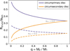 |
Fig. 1 Disc truncation radius in units of the binary semi-major axis as a function of the binary mass ratio (q) for the circumprimary (violet lines) and circumsecondary discs (orange lines). The solid lines correspond to a binary with ebin = 0, and the dashed lines indicate the case where ebin = 0.5. |
2.2 Evolution of the gas disc
We adopted the standard 1D axis-symmetric disc evolution model from the Bern Model and adapted it to the presence of the companion star by imposing that the outer disc edge is the tidal truncation radius given by Eqs. (1)–(3). The disc evolves by viscous accretion as well as by internal and external photoevaporation. The averaged gas surface density and viscosity at the disc midplane were used to solve the radial diffusion equation (Pringle 1981) with sink terms due to photoevaporation from the host star and planetary gas accretion. As in Zagaria et al. (2021), we adopted a zero-flux boundary condition at the truncation radius,
![Mathematical equation: $\[\begin{cases}\frac{\partial \Sigma_{\mathrm{gas}}}{\partial t}=\frac{3}{R} \frac{\partial}{\partial r}\left[r^{1 / 2} \frac{\partial}{\partial r}\left(v \Sigma_{\mathrm{gas}} r^{1 / 2}\right)\right]-\dot{\Sigma}_{\mathrm{photo}}(r)-\dot{\Sigma}_{\mathrm{planet}}(r),\\\qquad\qquad\qquad\qquad\qquad\qquad\qquad\quad\qquad\qquad \text { if } r \leq R_{\mathrm{trunc}},\\ \frac{\partial}{\partial r}\left(v \Sigma_{\mathrm{g}} r^{1 / 2}\right)=0 \quad \text { if } r=R_{\mathrm{trunc}}\end{cases}\]$](/articles/aa/full_html/2026/04/aa57243-25/aa57243-25-eq7.png) (4)
(4)
where t and r are the temporal and radial coordinates, Σgas is the gas surface density, and ν = αcsHg is the kinematic viscosity, given by the dimensionless parameter α (Shakura & Sunyaev 1973), the local sound speed (cs), and the disc scale height (Hg). ![Mathematical equation: $\[\dot{\Sigma}_{\text {photo}}(r)\]$](/articles/aa/full_html/2026/04/aa57243-25/aa57243-25-eq8.png) is the sink term due to the internal and external photoevaporation. The internal photoevaporation followed Clarke et al. (2001), while the external photoevaporation was modelled using the far-ultraviolet prescription of Matsuyama et al. (2003). We emphasise that we did not modify the photoevaporation rates compared to the nominal NGPPS series (Emsenhuber et al. 2021a). We discuss how external photoevaporation affects the disc lifetimes and its limiting role in the case of a disc truncated by a close secondary companion in Appendix B.
is the sink term due to the internal and external photoevaporation. The internal photoevaporation followed Clarke et al. (2001), while the external photoevaporation was modelled using the far-ultraviolet prescription of Matsuyama et al. (2003). We emphasise that we did not modify the photoevaporation rates compared to the nominal NGPPS series (Emsenhuber et al. 2021a). We discuss how external photoevaporation affects the disc lifetimes and its limiting role in the case of a disc truncated by a close secondary companion in Appendix B.
Vertical structure
The vertical structure of the disc was computed following the Bern Model in its version of Emsenhuber et al. (2021a), which employs the semi-analytical approach from Nakamoto & Nakagawa (1994) and Hueso & Guillot (2005). We adapted the equation for the disc midplane temperature by adding a term corresponding to the tidal heating stemming from the torque exerted by the stellar companion (Qtidal term), following Alexander et al. (2011). The disc midplane temperature is thus
![Mathematical equation: $\[\sigma T_{\mathrm{mid}}^4=\frac{1}{2}\left(\frac{3}{8} \tau_R+\frac{1}{2 \tau_P}\right) \dot{E}+\sigma T_{\mathrm{S}}^4+\left(1+\frac{1}{2 \tau_P}\right) \Sigma Q_{\text {tidal }},\]$](/articles/aa/full_html/2026/04/aa57243-25/aa57243-25-eq9.png) (5)
(5)
with Tmid the disc midplane temperature, TS the temperature due to the irradiation (see below), σ the Stefan-Boltzmann constant, τR and τP the Rosseland and Planck mean optical depths, respectively, and ![Mathematical equation: $\[\dot{E}\]$](/articles/aa/full_html/2026/04/aa57243-25/aa57243-25-eq10.png) the viscous dissipation rate. This formula yields the midplane temperature in the optically thick (the term with τR) and optically thin (the term with τP) regimes. The computation of
the viscous dissipation rate. This formula yields the midplane temperature in the optically thick (the term with τR) and optically thin (the term with τP) regimes. The computation of ![Mathematical equation: $\[\dot{E}\]$](/articles/aa/full_html/2026/04/aa57243-25/aa57243-25-eq11.png) , τR and τP is specified in Sect.3.2.1 of Emsenhuber et al. (2021a).
, τR and τP is specified in Sect.3.2.1 of Emsenhuber et al. (2021a).
The tidal heating term due to the torque exerted by the companion star is (Alexander et al. 2011)
![Mathematical equation: $\[Q_{\text {tidal }}=\left|\Omega_{\text {bin }}-\Omega(r)\right| \Lambda(r) \Sigma(r) d r\]$](/articles/aa/full_html/2026/04/aa57243-25/aa57243-25-eq12.png) (6)
(6)
and
![Mathematical equation: $\[\Lambda=-\frac{q^2 G M_1}{2 r}\left(\frac{r}{\Delta_p}\right)^4,\]$](/articles/aa/full_html/2026/04/aa57243-25/aa57243-25-eq13.png) (7)
(7)
where Δp = max(H, |r − abin|)
The irradiation temperature TS is calculated as
![Mathematical equation: $\[\begin{aligned}T_{\mathrm{S}}^4= & T_{\star, 1}^4\left[\frac{2}{3 \pi}\left(\frac{R_{\star, 1}}{r}\right)^3+\frac{1}{2}\left(\frac{R_{\star, 1}}{r}\right)^2 \frac{H}{r}\left(\frac{\partial \ln H}{\partial \operatorname{lnr}}-1\right)\right]+T_{\mathrm{irr}, 1}^4. \\& +T_{\mathrm{irr}, 2}^4+T_{\mathrm{min}, \text {disk.}}^4.\end{aligned}\]$](/articles/aa/full_html/2026/04/aa57243-25/aa57243-25-eq14.png) (8)
(8)
This expression is analogous to Eq.5 from Emsenhuber et al. (2021a), with quantities with the sub-index 1 referring to the primary star, and with 2 to the secondary star. The difference with Eq. (5) from Emsenhuber et al. (2021a) is that we not only considered the direct irradiation term through the disc midplane from the primary ![Mathematical equation: $\[T_{\mathrm{irr}, 1}^{4}\]$](/articles/aa/full_html/2026/04/aa57243-25/aa57243-25-eq15.png) , but from the secondary as well (
, but from the secondary as well (![Mathematical equation: $\[T_{\mathrm{irr}, 2}^{4}\]$](/articles/aa/full_html/2026/04/aa57243-25/aa57243-25-eq16.png) ). The term
). The term ![Mathematical equation: $\[T_{\mathrm{irr}, 1}^{4}\]$](/articles/aa/full_html/2026/04/aa57243-25/aa57243-25-eq17.png) is given by (Emsenhuber et al. 2021a, Eq. (6))
is given by (Emsenhuber et al. 2021a, Eq. (6))
![Mathematical equation: $\[T_{\mathrm{irr}, 1}^4=\frac{L_{\star, 1}}{16 \pi r^2 \sigma} e^{-\tau_{\mathrm{mid}}},\]$](/articles/aa/full_html/2026/04/aa57243-25/aa57243-25-eq18.png) (9)
(9)
where L⋆,1 is the primary luminosity, σ the Stefan-Boltzmann constant, and τmid the midplane optical depth, given by τmid = ∫ κ(r)ρ(r)dr, with the integral performed from the inner disc edge until the location r in the disc.
In the nominal Bern Model, Tmin,disk from Eq. (8) is the background temperature fixed at 10 K (Emsenhuber et al. 2021a). This term accounts for the heating by the surrounding environment (molecular cloud). In the presence of a stellar companion, beyond this background temperature is also the irradiation from the secondary star, which we included directly as ![Mathematical equation: $\[T_{\mathrm{irr}, 2}^{4}\]$](/articles/aa/full_html/2026/04/aa57243-25/aa57243-25-eq19.png) in Eq. (8). We note that this term could be complex if it is to be computed taking the disc and binary geometry into account, and also when a circumsecondary disc blocks the light from the secondary on its way to the circumprimary disc. Thus, we adopted a very simple approach. We only considered a direct irradiation term from the secondary to the circumprimary disc, at the midplane, and we only considered the equilibrium temperature that would emerge due to the irradiation from the secondary. Thus,
in Eq. (8). We note that this term could be complex if it is to be computed taking the disc and binary geometry into account, and also when a circumsecondary disc blocks the light from the secondary on its way to the circumprimary disc. Thus, we adopted a very simple approach. We only considered a direct irradiation term from the secondary to the circumprimary disc, at the midplane, and we only considered the equilibrium temperature that would emerge due to the irradiation from the secondary. Thus,
![Mathematical equation: $\[T_{\mathrm{irr}, 2}^4=\frac{L_{\star, 2}}{16 \pi r_2^2 \sigma} e^{-\tau_{\mathrm{mid}}^{\prime}},\]$](/articles/aa/full_html/2026/04/aa57243-25/aa57243-25-eq20.png) (10)
(10)
where r2 is the distance between the given location in the circumprimary disc and the secondary star, and L⋆,2 is the luminosity of the secondary star. For simplicity, we used the stellar mass-luminosity relation ![Mathematical equation: $\[L_{\star, 2} \sim M_{2}^{3.5}\]$](/articles/aa/full_html/2026/04/aa57243-25/aa57243-25-eq21.png) (normalised for the current solar luminosity). The optical depth
(normalised for the current solar luminosity). The optical depth ![Mathematical equation: $\[\tau_{\text {mid}}^{\prime}\]$](/articles/aa/full_html/2026/04/aa57243-25/aa57243-25-eq22.png) is analogous to τmid describe above, except that the integral is performed from the disc truncation radius to the inner disc edge. To compute r2, we used an average distance as for the computation of Δp in Eq. (7). We note that this term starts to be non-negligible when the luminosity of the secondary is of the same order as the luminosity of the primary star (i.e. binary mass ratios close to one).
is analogous to τmid describe above, except that the integral is performed from the disc truncation radius to the inner disc edge. To compute r2, we used an average distance as for the computation of Δp in Eq. (7). We note that this term starts to be non-negligible when the luminosity of the secondary is of the same order as the luminosity of the primary star (i.e. binary mass ratios close to one).
2.3 Evolution of the dust disc and pebble accretion
The solid accretion was assumed to be dominated by pebbles. To compute realistic pebble accretion rates, it is essential to properly compute the pebble sizes (Venturini et al. 2020b,a). To do this, we computed the dust evolution by coagulation, fragmentation, drift, and ice sublimation at the ice line. We adopted the two-population model from (Birnstiel et al. 2012), which describes the dust population by two dominant sizes: dust grains at a fixed size of 10−5 cm, and pebbles of evolving sizes. Dust and pebbles evolved embedded in the truncated gaseous discs presented in Sect. 2.1. The two-population model was introduced in the Bern Model by Voelkel et al. (2020). Unlike Voelkel et al. (2020), who used a single pebble fragmentation velocity for the entire disc, we adopted a fragmentation velocity in accordance with the pebble composition: vfrag = 1 m/s inside the ice line and vfrag = 10 m/s outside it (Blum 2018; Drążkowska & Alibert 2017; Guilera et al. 2020). For pebble accretion, we followed the prescription of Johansen & Lambrechts (2017) and incorporated the effect of halting pebble accretion when a planet reached the pebble isolation mass, as described by Lambrechts et al. (2014), and the effect of the planet eccentricity on the pebble accretion rate (Johansen & Lambrechts 2017, Eq. (36)).
3 Results
3.1 Gas-disc evolution
We first analysed the evolution of the gas disc for the nominal setup, defined by a disc with α = 10−3, an initial total disc mass before truncation of Md,0 = 0.1 M⊙, and an initial dust-to-gas ratio of 0.01. The binary parameters for this nominal setup were M1 = 1 M⊙, M2 = 0.5 M⊙, ebin = 0, and variable abin. All the simulations presented in this work assumed coplanarity between the binary and the protoplanetary disc. The initial conditions are also displayed for convenience in the middle column of Table 1, except that for the results of Sects. 3.1 and 3.2, we did not include the growth of any planet because we are interested in first understanding the disc evolution alone. Figure 2 shows the evolution of the surface density of gas (top panels) and of the midplane temperature as a function of radial distance to the primary for the cases where abin = 20 au (left panels) and abin = 100 au (right panels). The single-star case is shown for reference in the background. The disc disappears at 3.5 Myr for the single-star case, at 2.1 Myr for abin = 20 au, and at 4.3 Myr for abin = 100 au. The gap in the gas surface density at a few au that appears close to the disc dissipation is due to the effect of the internal photoevaporation, which more easily removes gas at intermediate distances (see, e.g. Venturini et al. 2020b).
Regarding the evolution of the disc midplane temperature, we note that the abin = 100 au case is very similar to the single-star case. On the other hand, for abin = 20 au, there is a considerable temperature increase close to the truncation radius when the binary is compared with the single-star case (increase in temperature from 70 K to 140 K for the first time step). This is the effect of the tidal heating from the stellar companion, and it is only noticeable for very close binaries and mainly at the beginning of the evolution.
The change in the temperature profile at r ~ 0.4–5 au is due to the water-ice line for all the cases. Icy grains indeed increase the disc opacity (modelled with the BL94 opacities), abating the drop in temperature with orbital distance. This change in slope moves inwards with time with the inner movement of the ice line as the disc cools down.
Table 2 displays the disc characteristics for the cases presented in Fig. 2, as well as for other binary separations. We note that the gas disc lifetimes do not always decrease when the binary separation is reduced, as might be intuitively expected because the more truncated the disc, the less massive it is, and thus, the easier it should be to remove the gas. The discs that we modelled, which stem from the nominal setup of the Bern Model, are discs whose evolution is driven by external photoevaporation. External photoevaporation produces discs that evolve outside-in (e.g. Coleman & Haworth 2022), that is, external photoevaporation efficiently removes material from the outer edge and drags gas along from the inner orbits until R≈20 au. When a disc is truncated within this radius, external photoevaporation cannot affect the disc evolution, rendering longer disc lifetimes. We analyse this effect in more depth in Appendix C.
In any case, we found that the limiting factor for planetary growth is not the gas disc lifetime, but the pebble disc lifetime. This was also reported by Zagaria et al. (2021). The pebbles disappear so quickly in truncated discs due to the fast radial drift and lack of a reservoir of dust farther out that the planetary seeds are quickly drained from solid material, preventing core growth. We analyse this in more detail below.
Disc properties for different binary separations for ebin = 0.
3.2 Dust disc evolution
Figure 3 shows the evolution of the surface density of pebbles (top panels) and of the pebble size along the disc for the nominal disc with abin = 20 au (left) and abin = 100 au (right). The grey background lines correspond to the single-star case. For all the cases, the abrupt increase in the pebble size when moving radially outwards, visible at r ~ 0.4–5 au, corresponds to the presence of the ice line. Icy pebbles have higher fragmentation velocities (see Sect. 2.3), and thus, they can grow to larger sizes than rocky pebbles. The change in the pebble size also affects the radial drift, with smaller rocky pebbles moving inwards slower. This creates the well-known pile-up of pebbles inside the ice line (e.g. Drązkowska et al. 2016), visible in the profiles of the pebble surface density in Fig. 3.
On the other hand, the peaks of pebbles towards the end of the disc dissipation emerge as a response to the gap in the gas midplane, carved by internal photoevaporation, as mentioned in Sect. 3.1. Nevertheless, it is particularly interesting to analyse the differences in the pebble evolution within the first time steps because the core growth by pebble accretion occurs very quickly, on timescales of ~105 years (see the next section, Fig. 4). When we compare the first time-snapshot of Fig. 3 (at time=105 years), we note that at r = 5 au, the surface density of pebbles is Σpeb = 10−2 g/cm2, while for the single-star case, it is Σpeb = 4 g/cm2. This is a reduction by a factor 400 for abin = 20 au compared to the single-star case after the first 105 years of disc evolution. This sharp drop in the pebble surface density is a consequence of the disc truncation and the loss of the outer reservoir of dust. As intuition dictates, the effect is less dramatic the larger the binary separation. For abin = 100 au, the effect is noticeable at the second time-snapshot (time=2 × 10⁵ years), where the surface density of pebbles for the truncated disc is Σpeb = 0.04 g/cm2 compared to Σpeb = 0.94 g/cm2 of the single-star case at r = 5 au (a drop by a factor 23.5 in this case).
The halting of the pebble supply also affects the pebble growth: the more truncated the disc, the smaller the pebbles at a given time, as illustrated in the bottom panels of Fig. 3. For the case of abin = 20 au, the situation is dramatic outside the ice line as we move towards Rtrunc, where the pebble size drops by a factor of 6 at r = 5 au and by a factor of 35 at r = 7 au compared to the single-star case within the first snapshot of the displayed evolution (time=105 years). The surface density of pebbles and the pebble sizes both affect the rate of pebble accretion to build the cores (Johansen & Lambrechts 2017). Thus, both effects play a detrimental role in the growth of the planetary cores, as we analyse in the next section.
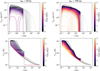 |
Fig. 2 Evolution of the gas disc as a function of orbital distance from the primary for the nominal disc with binary separations of abin = 20 au (left) and abin = 100 au (right). The grey background curves correspond to the single-star case. The disc profiles are shown every 105 years. The top panels display the evolution of the gas surface density, and the bottom panels show the evolution of the disc midplane temperature. |
3.3 Planetary growth
In this section, we analyse how a single Moon-mass embryo grows by pebble and gas accretion at fixed locations (no migration) in discs truncated by the tidal effect of a secondary star. We also show the single-star cases for reference. Figure 4 shows the growth at ap = 5 au and ap = 20 au for different binary separations and for the single-star case. We note that for all cases, the core completes its formation on a timescale of 105 years, while gas continues to be accreted until the disc dissipates (a few million years; see the corresponding disc characteristics in Table 2). After disc dissipation, the planet evolves by cooling and contracting at constant mass during gigayears.
For ap = 5 au (Figure 4, top panel) we note that a binary separation of 300 au produces the same planet as in the single-star case, and that we have to decrease the binary separation below 100 au to start to notice an effect on the planetary growth. We recall that for all the shown cases, the disc was truncated at Rtrunc ≈ 0.4 abin (see Fig. 1.) For ap = 20 au, we therefore cannot run cases with abin < 50 au because the planet would be beyond the outer disc edge.
For the planet growing at 5 au, the most dramatic effect on the planet growth is observed in the transition from abin = 75 to abin = 50 au, where the planet changes from reaching a mass of 80 M⊕ for abin = 75 to 0.4 M⊕ for abin = 50 au. For a planet located at 20 au, the strong drop in planet growth occurs between abin = 300 and abin = 100 au, where it transitions from a ~200 M⊕ planet for abin = 300 to an 0.5 Mars object for abin = 100 au. The detrimental effect on the planet growth for binary separations below approximately 50 au is thus evident in these examples. As we outlined in Sect. 3, this is not related to the gas disc lifetime, but to the dust disc lifetime. We note that for all our cases, when the surface density of pebbles drops below Σpeb ≤ 0.01 g/cm2, the pebble sizes reduce to values lower than apeb ≤ 0.5 cm (beyond the ice line), and the pebble accretion rates become negligible (![Mathematical equation: $\[\dot{M}_{\text {peb}} \leq 10^{-6} ~\mathrm{M}_{\oplus} / \mathrm{yr}\]$](/articles/aa/full_html/2026/04/aa57243-25/aa57243-25-eq23.png) ), halting planetary growth. Thus, the pebbles that are useful for building the cores are long gone by the time the discs are 1 Myr old (see again the evolution of Σpeb and of the pebble sizes along the discs in Fig. 3).
), halting planetary growth. Thus, the pebbles that are useful for building the cores are long gone by the time the discs are 1 Myr old (see again the evolution of Σpeb and of the pebble sizes along the discs in Fig. 3).
When we tried to quantify the exact transition between forming a giant planet versus a sub-Earth-mass object for different binary parameters, we note that this depends on the initial embryo location over the truncation radius, and that the clearest variable impacting this is the initial mass of solids in the disc. We show this in the following section.
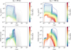 |
Fig. 3 Evolution of the pebble disc as function of orbital distance from the primary for the nominal disc with binary separations of abin = 20 au (left) and abin = 100 au (right). The grey background curves correspond to the single-star case. The disc profiles are shown every 105 years. The top panels indicate the evolution of the pebble surface density, and the bottom panels show the evolution of the pebble sizes. The abrupt change in the pebble size at r ~ 0.4–5 au for all the profiles and times corresponds to the location of the water-ice line. This also affects the profiles of the pebble surface density. |
3.4 Parameter study
To investigate how the reduced material supply caused by disc truncation affects the planet growth across a variety of binary configurations, we carried out a grid of 5000 simulations. We fixed the mass of the primary star, M1, at 1 M⊙ and randomly drew the secondary star’s mass, M2, between 0.1 and 1 M⊙, to sample a broad range of binary mass ratios q. The binary separation abin and eccentricity ebin were randomly sampled within the ranges 10–1000 au, and 0–0.9, respectively. In each simulation, we modelled the in situ growth of a single Moon-mass embryo (i.e. Mp = 10−2 M⊕), placed at a location ap,0 randomly chosen between 1 au and the location of the truncation radius Rtrunc minus 1 au. We also sampled the initial disc mass, Md,0, between 10−3 M⊙ and 0.1 M⊙, the dust-to-gas ratio, fD/G, between 0.0056 and 0.03162, the disc viscosity, α, between 10−4 and 10−3, and the disc characteristic radius, rc, between 10 au and 200 au. These chosen ranges were physically motivated by observational data of single-star discs and were used by Emsenhuber et al. (2021b) and Weder et al. (2023). All these parameters were sampled with a uniform or log-uniform distribution, and we summarise these initial conditions in the right column of Table 1.
In Figure 5, we show the output of the planet formation simulations as a function of the binary mass ratio and binary separation (top panel) or truncation radius (bottom panel). In both panels, each circle is a planet, for which the final planet mass is indicated in the colour bar. For better visualisation, we only display systems that formed planets more massive than Mars. The shaded purple contours mark areas of highest number density for planets with masses greater than 10 M⊕.
An important science question to address is which type of planets forms for different binary separations. We find that planets more massive than Mars form practically everywhere for all abin > 13 au, when it is assumed that each log-bin of binary separation in the range 10 < abin < 1000 au is equally likely to produce planets. Nevertheless, we note that planets more massive than 10 M⊕ form for abin > 33.5 au, while giant planets with MP > 100 M⊕ form for abin > 40.6 au. These results hold regardless of the binary mass ratio (q) and for all the binary eccentricities considered (ebin < 0.9). The are some specific trends in the final planet masses that depend on ebin, but we analyse this effect in detail in Paper II.
Another relevant aspect to analyse is the suppression of planet formation for decreasing binary separations. How does this operate when considering only the effect of tidal disc truncation? The answer is shown in Fig. 6. It shows that when all the planets more massive than Mars are considered, their formation becomes steadily suppressed for abin < 160 au. On the other hand, for planets more massive than 10 M⊕, their suppression is noticeable for abin < 600 au. It is interesting to see that the number of small S-type planets drops mildly for abin > 160 au, while the number of giant planets continues to rise for increasing abin, up to abin ~ 600 au. The larger the binary separation, the more extended the discs, and thus, cores can accrete more solids, which leads to the formation of more giants (and thus, fewer small planets). Thus, our results suggest that the answer to the question of planet formation suppression in binaries depends on the planet mass range that is analysed: giant planet formation is suppressed at larger binary separations than the formation of small planets. This aspect might explain the different findings of Lester et al. (2021) and Thebault & Bonanni (2025).
As a word of caution, it is important to emphasise that these results hold under the assumption of an initial log-uniform distribution in abin, which is not the observed distribution of binary separations in field binaries (Raghavan et al. 2010). The purpose of this exercise is simply to analyse the effect of tidal disc truncation alone on the suppression of the formation of (single-embryo) S-type planets, when assuming all binary separations to be equally likely to produce planets. In addition, the gravitational perturbation from the secondary star is not included in these calculations, nor is orbital migration. Thus, these numbers should not be directly compared to observations. We will present proper occurrence rates in a future population synthesis study (Paper III; Nigioni et al. 2026.)
As discussed in Section 3.3, S-type planet formation depends not only on the binary properties, but also on the planet location. In particular, planets more massive than Mars only form when they are located within 28% of the binary separation, with 75% of them being concentrated at only 4% of the abin (Fig. 7, top panel). In terms of disc truncation, planets more massive than Mars are located at ap,0/Rtrunc < 0.85, with 75% of them being concentrated at the innermost 22% of the truncated disc (Fig. 7, bottom panel). When focusing on more massive planets, we note that they are slightly closer in: for MP > 10 M⊕, ap,0/Rtrunc ≲ 0.71 and for MP > 100, ap,0/Rtrunc ≲ 0.61. We note that in the illustrative examples of Fig. 4, for the formation location of ap,0 = 5 au (top panel), the giant planet that forms for abin = 75 au indeed has ap,0/Rtrunc = 0.19, while for the one forming at ap,0 = 20 au, and abin = 300 au, ap,0/Rtrunc = 0.172 (disc truncation values taken from Table 2). When we consider the different variables that we analysed to understand the output of planet formation (see Figs. 5 and 7), the initial mass of solids in the disc seems to be the clearest quantity influencing the final planet mass (Fig. 7). This a fundamental result of the core accretion model, also reported in the past for single stars (Mishra et al. 2023). For S-type planets, the initial mass of solids in the disc is directly linked to the truncation radius, which depends linearly on abin (see Eq. (1)).
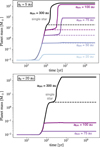 |
Fig. 4 In situ planet growth by pebble accretion at ap = 5 au (top panel) and ap = 20 au (bottom panel). The solid lines indicate the evolution of the total planet mass, and the dashed lines show the evolution of the core mass. The different colours correspond to different binary separations, as indicated in the labels. After the final planet mass is reached during the disc lifetime (a few million years), the planet evolves during gigayears by cooling and contraction. |
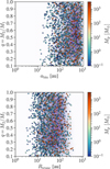 |
Fig. 5 Binary mass ratio vs. binary separation (top panel) and binary mass ratio vs. disc truncation radius (bottom panel) for systems that formed a planet at least more massive than Mars. The colour bar indicates the final planet mass. The shaded contour regions represent areas with the highest number planet density, derived from a two-dimensional KDE performed on planets with masses greater than 10 M⊕. The lack of planets for Rtrunc>400 au stems from the choice of the upper limit on abin = 1000 au (see Table 1). |
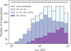 |
Fig. 6 Number of formed S-type planets as a function of binary semi-major axis (abin) from the grid of 5000 simulations presented in Sect. 3.4. The dashed black line illustrates the log-uniform distribution of abin adopted as the initial condition (multiplied by 0.5 for better visualisation). The different colours of the bars correspond to different ranges of planet mass, indicated in the legend of the figure. The simulations assumed one embryo per disc and did not include the gravitational perturbation from the secondary or orbital migration. |
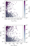 |
Fig. 7 Initial planet location relative to the binary separation, ap,0/abin, vs. final planet mass (top panel) and initial planet location relative to the disc truncation radius, ap,0/Rtrunc, vs. final planet mass (bottom panel) for systems that formed a planet at least more massive than Mars. The colour bar indicates the initial mass of solids in the disc after truncation. The x-axis scale is different in each plot. |
4 Discussion
4.1 The non-formation of γ-Cephei-like planets
One of the best known cases of an S-type binary is γ-Cephei, an extreme S-type system with M1 ≈ 1.3 M⊙, M2 ≈ 0.33 M⊙ (binary mass ratio of q≈0.26), a binary separation of abin ≈ 20 au, binary eccentricity of ebin ≈0.4, hosting a 6.6 Jupiter-mass planet orbiting the primary star at 2 au (Hatzes et al. 2003; Knudstrup et al. 2023). The disc of γ-Cephei should have been truncated at Rtrunc ≈ 4.4 au (for α = 10−3), according to the prescription presented in Sect. 2. Different works have explored the formation, dynamical evolution, and long-term stability of γ-Cephei and generally agreed that it is very challenging to explain the formation of its giant planet (Thébault et al. 2004; Kley & Nelson 2008; Jang-Condell et al. 2008; Müller & Kley 2012; Jordan et al. 2021). The main difficulty for reproducing the γ-Cephei planet is the severe disc truncation by the eccentric stellar companion, which notably reduces the available mass of gas and dust to form the giant planet (Kley & Nelson 2008; Zagaria et al. 2021). Hydrodynamical simulations suggest that the circumprimary disc can develop a significant eccentricity (Kley et al. 2008; Marzari et al. 2009, 2012; Müller & Kley 2012), which, combined with gravitational perturbations from the secondary star, might increase planetesimal relative velocities and lead to destructive rather than accretional collisions (Paardekooper et al. 2008). However, Beaugé et al. (2010) found that for high disc eccentricities, disc precession can instead reduce the velocity dispersion between different-size planetesimals, favouring accretional collisions in the outer disc regions.
The formation of planets in binary systems, particularly in systems like γ-Cephei, has not yet been explored in the context of pebble accretion. In this first work, we addressed this gap by modelling planet formation under this paradigm. While this first approach simplifies certain aspects, such as the omission of detailed binary dynamics and planet migration, it provides valuable insights. Our results, especially those presented in Sect. 3.4, show that pebble accretion on its own can form a gas giant (MP > 100 M⊕) for abin ≳ 40 au and Rtrunc ≳ 7 au. This means that we cannot strictly form a γ-Cephei-like planet with the current model. Nevertheless, it seems that we are not far from forming a giant planet with the expected truncation radius of γ-Cephei. Some of our simulations produced cores of 2–5 M⊕ for Rtrunc ≈ 2–7 au. With a slightly different history of solid accretion or envelope opacity, these cores might enter the runaway gas phase. Furthermore, the mass of the primary in γ-Cephei is 30% higher than solar, meaning that more solids might have been present in the disc of γ-Cephei compared to the values considered in our simulations (solar-mass primaries). Thus, our simulations offer a starting point for a deeper exploration of the initial conditions and physical parameters that might lead to the formation of γ-Cephei Ab. We will address this in the future.
Another potential solution to overcome the γ-Cephei problem has recently been proposed by Marzari & D’Angelo (2025). The authors suggested that the system might have hosted an extended circumbinary disc, a remnant of the stellar formation process, that might have acted as a reservoir that supplied both gas and solids to the circumprimary disc. Through high-resolution hydrodynamical simulations, the authors showed that in a γ-Cephei like system, gas can be supplied by the outer circumbinary disc to the circumprimary disc, extending its lifetime for up to ~3 Myr (about three times the lifetime of the same disc in isolation). Moreover, Marzari & D’Angelo (2025) showed that solids can also be transported to the circumprimary disc. This mechanism might thereby have important implications for planet formation in close binaries, and we will examine it in a follow-up study (Ronco et al. in prep.). Extremely tight S-type binaries might undergo a different formation path, as suggested by Marzari & D’Angelo (2025), albeit more work is needed to quantify the binary parameters for which this scenario might work.
Finally, another formation pathway for γ-Cephei Ab might be gravitational instability (GI), which proposes that planets form through the rapid collapse of gas into self-gravitating clumps in sufficiently massive protoplanetary discs. For fragmentation to occur, however, the disc must cool efficiently so that self-gravity overcomes pressure support, a condition that is generally only met at large distances from the star (Boss 1998, 2002; Rafikov 2005). Thus, invoking GI as the formation pathway for γ-Cephei Ab (or for planets in relatively close binaries in general) might be challenging for the physical properties of tidally truncated discs. As we showed, discs in close binary systems are expected to be significantly less massive than around single stars due to the truncation of their outer regions, preventing them from reaching the higher surface densities necessary for fragmentation to occur. In addition, these truncated discs are typically hotter than discs around single stars, reducing their ability to cool quickly enough for GI to operate. Although Duchêne (2010) suggested that truncated discs might become more gravitationally unstable and that perturbations from the companion might help trigger collapse, other numerical studies found the opposite trend: dynamical perturbations from the secondary can actually suppress gravitational instabilities (see Mayer et al. 2010, and references therein). Last, the metallicity of γ-Cephei is super-solar, [Fe/H]≈+0.20 dex. This aspect is typically linked to the prevalence of the coreaccretion scenario for the formation of giant planets (Santos et al. 2004). Thus, taken together, these considerations probably make GI an unlikely formation pathway for γ-Cephei-like planets.
It is worth to emphasise that in any case, γ-Cephei systems are rare: giant S-type planets with abin < 100 au have an estimated occurrence rate of 4% (Hirsch et al. 2021), and they represent fewer than 2% of the sample of S-type planets in the catalog of Thebault & Bonanni (2025). Thus, although understanding their formation poses an interesting theoretical challenge, the main aim of global models and population synthesis is to reproduce observed demographic trends (which we do fairly well, as we will present in Paper III), and not specific systems.
4.2 Model limitations
One limitation of this work is the absence of a model for the potential disc photo-evaporation driven by the secondary star. This effect might be relevant in close binary systems, where irradiation from the secondary might still affect the outer regions of the primary disc. As noted by Rosotti & Clarke (2018), full 3D simulations are required to accurately capture this phenomenon. Nevertheless, we can attempt a rough estimate of the EUV photoevaporation rate by adapting the extreme-UV (EUV) mass-loss rate prescription of Matsuyama et al. (2003) for external photoevaporation from nearby O/B stars. In their Eq. (16), the EUV mass-loss rate depends on the outer disc edge, on the ionization rate of the external star, and on the distance to the external star. They considered the distance as that between the dominant star in the Trapezium cluster, θ1 Ori C, and the proplyds in it, which is about 0.03 pc, and the ionisation rate of θ1 Ori C, which is ~1049 s−1. In our context, we can obtain a rough estimate by using the binary separation as the relevant distance, the ionisation rate usually considered for Sun-like stars, which is ~ 1041 s−1, and the disc edge as the disc truncation radius. This gives a very low ![Mathematical equation: $\[\dot{M}_{\mathrm{d}}^{\text {EUV}} \sim 1 \times 10^{-10} ~M_{\odot} / \mathrm{yr}\]$](/articles/aa/full_html/2026/04/aa57243-25/aa57243-25-eq24.png) , which would affect the most external part of the disc only very little.
, which would affect the most external part of the disc only very little.
Concerning 3D additional effects, we note that out simple 1D disc model cannot capture asymmetric effects such as asymmetric irradiation or episodic outburst from the companion. This 100 yr timescale effect might reset the initial conditions for very close binaries (Poblete et al. 2025). Another hydrodynamic effect that we cannot capture is the appearance of spiral arms (Kley et al. 2008), which might act as local dust traps for planetesimal formation. This effect deserves further investigation within the context of S-type planet formation.
Regarding the model setup, for the sake of isolating the effect of the disc truncation on the planet growth by pebble accretion, we only considered in situ growth of a single embryo here. The effect of orbital migration is analysed in Paper II, and it is also the default setup for the population synthesis of the upcoming Paper III. We mention here that inward migration just moves the protoplanet to a region in which the supply of pebbles lasts longer. This is in principle beneficial for the core growth, but in reality, if the protoplanet moves inside the ice line, then the pebble accretion rate drops due to the decrease in the pebble size. Another interesting effect to discuss is how the growth of one planet influences the growth of subsequent planets. In the simulations we presented in Sect. 3.3, we note that for the cases in which a giant planet formed, the gap created in the disc produced a density maximum farther out that acted as a pebble-collector (e.g. Guilera & Sándor 2017; Guilera et al. 2020). We show this in Fig. 8, which is the same as we presented in the top right panel of Fig. 3, but considering in this case the growing planet at r=5 au (and its feedback on the disc structure). We note that the pebbles accumulate in the density maximum at r≈ 10 au. This might be a way to retain more pebbles in the disc and trigger subsequent farther out planet formation (as already suggested for single stars by Lau et al. 2024). Giant planets are expected to have outer planet siblings, also in binaries.
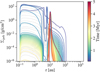 |
Fig. 8 Same as Figure 3 for the abin = 100 au case (and single-star in the grey background), but taking into account the growth of the giant planet at 5 au and the feedback of it on the disc. The evolution of the planet mass is shown in Fig. 4 for the binary and single-star cases. |
5 Conclusions
We introduced the project Planet formation Around bInaRy Stars, PAIRS, which aims to develop the first global formation model for planets orbiting binary stars suited for planet population synthesis. In this first paper, we presented the adaptation of the circumstellar disc to an external stellar companion to simulate the formation of S-type planets by pebble accretion. We included the physical effects of tidal disc truncation and heating and the direct irradiation from the stellar companion in the evolution of a circumstellar disc that undergoes viscous accretion and internal and external photoevaporation. The results of this study do not include the gravitational perturbation from the stellar companion on the planetary bodies. This is presented in the accompanying Paper II (Nigioni et al. 2026).
We provide an open source script to compute the outer truncation radius of an S-type disc for any binary parameter (see Sect. 2.1) based on the fits from Manara et al. (2019) to the analytical results of Artymowicz & Lubow (1994). The disc truncation radius depends on the binary semi-major axis, binary eccentricity, binary mass ratio, and assumed disc viscosity. The circumprimary and circumsecondary disc truncation radius can be computed with the provided tool.
We additionally studied how a planetary embryo grows in situ in these truncated discs by the accretion of pebbles and gas. We analysed the dependence of the planet growth on different binary parameters, spanning binary separations sampled log-uniformly from 10 to 1000 au, and binary mass ratios from 0.1 to 1. We found that S-type planets attaining a mass higher than Mars form in the whole range of the adopted binary separations, but we note that planet formation is steadily suppressed for abin < 160 au. (Fig. 6). The main cause of this detrimental effect on planet formation is the cut-off of the pebble supply from the outer disc due to disc truncation, which starves the growth of the cores (Sects. 3.2 and 3.3). In terms of disc truncation, planets more massive than Mars form for Rtrunc ≳ 3 au, while the lower limit for planets with MP > 10 M⊕ is Rtrunc ≈ 7 au (Fig. 5). We also found that S-type planets typically form close to their central star in relation to the binary separation and to the disc truncation radius: 75% of planets more massive than Mars form at ap,0/abin<4% and ap,0/Rtrunc < 22%. No planet forms for ap,0/abin > 30% or ap,0/Rtrunc > 85%. This is also a consequence of the disc tidal truncation: the closer the planet to the disc truncation radius, the sooner the supply from pebbles stops, halting core growth.
Overall, we showed for the first time that pebble accretion allows for the formation of S-type planets, and we quantified the detrimental effect on planet growth for close binaries when considering the effect of tidal disc truncation. We analyse the added effect of the gravitational perturbation from the stellar companion in the accompanying Paper II, and we will present the results of the first S-type planet population synthesis in Paper III.
Data availability
The data corresponding to the grid of 5000 simulations is available on Zenodo at this link: https://doi.org/10.5281/zenodo.18889347.
Acknowledgements
We thank the referee for a very constructive and insightful report that helped us to improve the presentation of the results and discussions. We thank C. Mordasini, A. Kessler, J. Weder and R. Burn for valuable discussions about the Bern Model. J.V. and A.N. acknowledge support from the Swiss National Science Foundation (SNSF) under grant PZ00P2_208945. MPR is partially supported by PIP-2971 from CONICET (Argentina) and by PICT 2020-03316 from Agencia I+D+i (Argentina). This work has been carried out within the framework of the NCCR PlanetS supported by the Swiss National Science Foundation. The computations were performed at University of Geneva on the Yggdrasil cluster. This research has made use of NASA’s Astrophysics Data System. Software. For this publication the following software packages have been used: Python-matplotlib by Hunter (2007), Python-seaborn by Waskom & the seaborn development team (2020), Python-numpy, Python-pandas.
References
- Alexander, R. D., Wynn, G. A., King, A. R., & Pringle, J. E. 2011, MNRAS, 418, 2576 [Google Scholar]
- Alibert, Y., & Venturini, J. 2019, A&A, 626, A21 [NASA ADS] [CrossRef] [EDP Sciences] [Google Scholar]
- Alibert, Y., Mordasini, C., Benz, W., & Winisdoerffer, C. 2005, A&A, 434, 343 [NASA ADS] [CrossRef] [EDP Sciences] [Google Scholar]
- Artymowicz, P., & Lubow, S. H. 1994, ApJ, 421, 651 [Google Scholar]
- Barenfeld, S. A., Carpenter, J. M., Sargent, A. I., et al. 2019, ApJ, 878, 45 [Google Scholar]
- Beaugé, C., Leiva, A. M., Haghighipour, N., & Otto, J. C. 2010, MNRAS, 408, 503 [Google Scholar]
- Behmard, A., Dai, F., & Howard, A. W. 2022, AJ, 163, 160 [NASA ADS] [CrossRef] [Google Scholar]
- Bell, K. R., & Lin, D. N. C. 1994, ApJ, 427, 987 [NASA ADS] [CrossRef] [Google Scholar]
- Benz, W., Ida, S., Alibert, Y., Lin, D., & Mordasini, C. 2014, Protostars and Planets VI, 691 [Google Scholar]
- Birnstiel, T., Klahr, H., & Ercolano, B. 2012, A&A, 539, A148 [NASA ADS] [CrossRef] [EDP Sciences] [Google Scholar]
- Blum, J. 2018, Space Sci. Rev., 214, 52 [NASA ADS] [CrossRef] [Google Scholar]
- Bodenheimer, P., D’Angelo, G., Lissauer, J. J., Fortney, J. J., & Saumon, D. 2013, ApJ, 770, 120 [NASA ADS] [CrossRef] [Google Scholar]
- Bodenheimer, P., Hubickyj, O., & Lissauer, J. J. 2000, Icarus, 143, 2 [Google Scholar]
- Bolmont, E., & Mathis, S. 2016, Celest. Mech. Dyn. Astron., 126, 275 [Google Scholar]
- Boss, A. P. 1998, ApJ, 503, 923 [Google Scholar]
- Boss, A. P. 2002, ApJ, 576, 462 [Google Scholar]
- Chambers, J. E., Quintana, E. V., Duncan, M. J., & Lissauer, J. J. 2002, AJ, 123, 2884 [NASA ADS] [CrossRef] [Google Scholar]
- Clarke, C. J., Gendrin, A., & Sotomayor, M. 2001, MNRAS, 328, 485 [NASA ADS] [CrossRef] [Google Scholar]
- Coleman, G. A. L., & Haworth, T. J. 2022, MNRAS, 514, 2315 [NASA ADS] [CrossRef] [Google Scholar]
- Doyle, L. R., Carter, J. A., Fabrycky, D. C., et al. 2011, Science, 333, 1602 [NASA ADS] [CrossRef] [Google Scholar]
- Drążkowska, J., & Alibert, Y. 2017, A&A, 608, A92 [Google Scholar]
- Drązkowska, J., Alibert, Y., & Moore, B. 2016, A&A, 594, A105 [CrossRef] [EDP Sciences] [Google Scholar]
- Drążkowska, J., Stammler, S. M., & Birnstiel, T. 2021, A&A, 647, A15 [Google Scholar]
- Duchêne, G. 2010, ApJ, 709, L114 [Google Scholar]
- Eggleton, P. P. 1983, ApJ, 268, 368 [Google Scholar]
- Emsenhuber, A., Mordasini, C., Burn, R., et al. 2021a, A&A, 656, A69 [NASA ADS] [CrossRef] [EDP Sciences] [Google Scholar]
- Emsenhuber, A., Mordasini, C., Burn, R., et al. 2021b, A&A, 656, A70 [NASA ADS] [CrossRef] [EDP Sciences] [Google Scholar]
- Fontanive, C., & Bardalez Gagliuffi, D. 2021, Front. Astron. Space Sci., 8, 16 [NASA ADS] [CrossRef] [Google Scholar]
- Fortier, A., Alibert, Y., Carron, F., Benz, W., & Dittkrist, K.-M. 2013, A&A, 549, A44 [NASA ADS] [CrossRef] [EDP Sciences] [Google Scholar]
- Freedman, R. S., Lustig-Yaeger, J., Fortney, J. J., et al. 2014, ApJS, 214, 25 [CrossRef] [Google Scholar]
- Giuppone, C. A., Leiva, A. M., Correa-Otto, J., & Beaugé, C. 2011, A&A, 530, A103 [NASA ADS] [CrossRef] [EDP Sciences] [Google Scholar]
- Guilera, O. M., & Sándor, Z. 2017, A&A, 604, A10 [Google Scholar]
- Guilera, O. M., Sándor, Z., Ronco, M. P., Venturini, J., & Miller Bertolami, M. M. 2020, A&A, 642, A140 [NASA ADS] [CrossRef] [EDP Sciences] [Google Scholar]
- Haghighipour, N. 2006, ApJ, 644, 543 [Google Scholar]
- Hatzes, A. P., Cochran, W. D., Endl, M., et al. 2003, ApJ, 599, 1383 [NASA ADS] [CrossRef] [Google Scholar]
- Hirsch, L. A., Rosenthal, L., Fulton, B. J., et al. 2021, AJ, 161, 134 [NASA ADS] [CrossRef] [Google Scholar]
- Hueso, R., & Guillot, T. 2005, A&A, 442, 703 [NASA ADS] [CrossRef] [EDP Sciences] [Google Scholar]
- Hunter, J. D. 2007, Comput. Sci. Eng., 9, 90 [NASA ADS] [CrossRef] [Google Scholar]
- Ida, S., & Lin, D. N. C. 2004, ApJ, 604, 388 [Google Scholar]
- Jang-Condell, H., Mugrauer, M., & Schmidt, T. 2008, ApJ, 683, L191 [NASA ADS] [CrossRef] [Google Scholar]
- Jin, S., Mordasini, C., Parmentier, V., et al. 2014, ApJ, 795, 65 [Google Scholar]
- Johansen, A., & Lambrechts, M. 2017, Annu. Rev. Earth Planet. Sci., 45, 359 [Google Scholar]
- Johnstone, C. P., Bartel, M., & Güdel, M. 2021, A&A, 649, A96 [EDP Sciences] [Google Scholar]
- Jordan, L. M., Kley, W., Picogna, G., & Marzari, F. 2021, A&A, 654, A54 [NASA ADS] [CrossRef] [EDP Sciences] [Google Scholar]
- Kley, W., & Haghighipour, N. 2014, A&A, 564, A72 [NASA ADS] [CrossRef] [EDP Sciences] [Google Scholar]
- Kley, W., & Nelson, R. P. 2008, A&A, 486, 617 [NASA ADS] [CrossRef] [EDP Sciences] [Google Scholar]
- Kley, W., Papaloizou, J. C. B., & Ogilvie, G. I. 2008, A&A, 487, 671 [NASA ADS] [CrossRef] [EDP Sciences] [Google Scholar]
- Kley, W., Thun, D., & Penzlin, A. B. T. 2019, A&A, 627, A91 [NASA ADS] [CrossRef] [EDP Sciences] [Google Scholar]
- Knudstrup, E., Lund, M. N., Fredslund Andersen, M., et al. 2023, A&A, 675, A197 [NASA ADS] [CrossRef] [EDP Sciences] [Google Scholar]
- Kostov, V. B., Orosz, J. A., Feinstein, A. D., et al. 2020, AJ, 159, 253 [Google Scholar]
- Kostov, V. B., Powell, B. P., Orosz, J. A., et al. 2021, AJ, 162, 234 [NASA ADS] [CrossRef] [Google Scholar]
- Kutra, T., Prato, L., Tofflemire, B. M., et al. 2025, AJ, 169, 20 [Google Scholar]
- Lambrechts, M., & Johansen, A. 2012, A&A, 544, A32 [NASA ADS] [CrossRef] [EDP Sciences] [Google Scholar]
- Lambrechts, M., & Johansen, A. 2014, A&A, 572, A107 [NASA ADS] [CrossRef] [EDP Sciences] [Google Scholar]
- Lambrechts, M., Johansen, A., & Morbidelli, A. 2014, A&A, 572, A35 [NASA ADS] [CrossRef] [EDP Sciences] [Google Scholar]
- Lau, T. C. H., Birnstiel, T., Drążkowska, J., & Stammler, S. M. 2024, A&A, 688, A22 [NASA ADS] [CrossRef] [EDP Sciences] [Google Scholar]
- Lester, K. V., Matson, R. A., Howell, S. B., et al. 2021, AJ, 162, 75 [NASA ADS] [CrossRef] [Google Scholar]
- Lester, K. V., Howell, S. B., Ciardi, D. R., & Matson, R. A. 2022, AJ, 164, 56 [NASA ADS] [CrossRef] [Google Scholar]
- Lissauer, J. J., Hubickyj, O., D’Angelo, G., & Bodenheimer, P. 2009, Icarus, 199, 338 [NASA ADS] [CrossRef] [Google Scholar]
- Manara, C. F., Tazzari, M., Long, F., et al. 2019, A&A, 628, A95 [NASA ADS] [CrossRef] [EDP Sciences] [Google Scholar]
- Martin, D. V. 2018, in Handbook of Exoplanets, eds. H. J. Deeg, & J. A. Belmonte, 156 [Google Scholar]
- Marzari, F., & D’Angelo, G. 2025, A&A, 695, A53 [NASA ADS] [CrossRef] [EDP Sciences] [Google Scholar]
- Marzari, F., & Scholl, H. 2000, ApJ, 543, 328 [NASA ADS] [CrossRef] [Google Scholar]
- Marzari, F., & Thebault, P. 2019, Galaxies, 7, 84 [NASA ADS] [CrossRef] [Google Scholar]
- Marzari, F., Scholl, H., Thébault, P., & Baruteau, C. 2009, A&A, 508, 1493 [NASA ADS] [CrossRef] [EDP Sciences] [Google Scholar]
- Marzari, F., Baruteau, C., Scholl, H., & Thebault, P. 2012, A&A, 539, A98 [NASA ADS] [CrossRef] [EDP Sciences] [Google Scholar]
- Matsuyama, I., Johnstone, D., & Hartmann, L. 2003, ApJ, 582, 893 [NASA ADS] [CrossRef] [Google Scholar]
- Mayer, L., Boss, A., & Nelson, A. F. 2010, Gravitational Instability in Binary Protoplanetary Disks, ed. N. Haghighipour (Dordrecht: Springer Netherlands), 195 [Google Scholar]
- Migaszewski, C. 2015, MNRAS, 453, 1632 [Google Scholar]
- Mishra, L., Alibert, Y., Udry, S., & Mordasini, C. 2023, A&A, 670, A69 [NASA ADS] [CrossRef] [EDP Sciences] [Google Scholar]
- Mordasini, C., Alibert, Y., & Benz, W. 2009, A&A, 501, 1139 [CrossRef] [EDP Sciences] [Google Scholar]
- Mordasini, C., Alibert, Y., Georgy, C., et al. 2012a, A&A, 547, A112 [NASA ADS] [CrossRef] [EDP Sciences] [Google Scholar]
- Mordasini, C., Alibert, Y., Klahr, H., & Henning, T. 2012b, A&A, 547, A111 [NASA ADS] [CrossRef] [EDP Sciences] [Google Scholar]
- Mordasini, C., Klahr, H., Alibert, Y., Miller, N., & Henning, T. 2014, A&A, 566, A141 [NASA ADS] [CrossRef] [EDP Sciences] [Google Scholar]
- Mordasini, C., Mollière, P., Dittkrist, K. M., Jin, S., & Alibert, Y. 2015, Int. J. Astrobiol., 14, 201 [NASA ADS] [CrossRef] [Google Scholar]
- Moutou, C., Petit, P., Charpentier, P., et al. 2026, A&A, 705, A190 [NASA ADS] [CrossRef] [EDP Sciences] [Google Scholar]
- Movshovitz, N., & Podolak, M. 2008, Icarus, 194, 368 [NASA ADS] [CrossRef] [Google Scholar]
- Mugrauer, M. & Michel, K.-U. 2021, Astron. Nachr., 342, 840 [NASA ADS] [CrossRef] [Google Scholar]
- Mugrauer, M., Zander, J., & Michel, K.-U. 2022, Astron. Nachr., 343, e24017 [NASA ADS] [Google Scholar]
- Mugrauer, M., Rück, J., & Michel, K. U. 2023, Astron. Nachr., 344, e20230055 [Google Scholar]
- Müller, T. W. A., & Kley, W. 2012, A&A, 539, A18 [Google Scholar]
- Nakamoto, T., & Nakagawa, Y. 1994, ApJ, 421, 640 [Google Scholar]
- Nelson, R. P. 2003, MNRAS, 345, 233 [NASA ADS] [CrossRef] [Google Scholar]
- Nigioni, A., Venturini, J., Bolmont, E., et al. 2026, A&A, 708, A38 [NASA ADS] [CrossRef] [EDP Sciences] [Google Scholar]
- Ormel, C. W., & Klahr, H. H. 2010, A&A, 520, A43 [NASA ADS] [CrossRef] [EDP Sciences] [Google Scholar]
- Paardekooper, S. J., Thébault, P., & Mellema, G. 2008, MNRAS, 386, 973 [NASA ADS] [CrossRef] [Google Scholar]
- Papaloizou, J., & Pringle, J. E. 1977, MNRAS, 181, 441 [NASA ADS] [CrossRef] [Google Scholar]
- Papaloizou, J. C. B., & Terquem, C. 1999, ApJ, 521, 823 [NASA ADS] [CrossRef] [Google Scholar]
- Poblete, P. P., Cuello, N., Alaguero, A., et al. 2025, A&A, 703, A76 [NASA ADS] [CrossRef] [EDP Sciences] [Google Scholar]
- Pringle, J. E. 1981, ARA&A, 19, 137 [Google Scholar]
- Quintana, E. V., & Lissauer, J. J. 2006, Icarus, 185, 1 [NASA ADS] [CrossRef] [Google Scholar]
- Quintana, E. V., Adams, F. C., Lissauer, J. J., & Chambers, J. E. 2007, ApJ, 660, 807 [Google Scholar]
- Rafikov, R. R. 2005, ApJ, 621, L69 [Google Scholar]
- Rafikov, R. R., & Silsbee, K. 2015b, ApJ, 798, 70 [Google Scholar]
- Rafikov, R. R., & Silsbee, K. 2015a, ApJ, 798, 69 [Google Scholar]
- Raghavan, D., McAlister, H. A., Henry, T. J., et al. 2010, ApJS, 190, 1 [Google Scholar]
- Rao, S., Meynet, G., Eggenberger, P., et al. 2018, A&A, 618, A18 [NASA ADS] [CrossRef] [EDP Sciences] [Google Scholar]
- Ronco, M. P., Guilera, O. M., Cuadra, J., et al. 2021, ApJ, 916, 113 [NASA ADS] [CrossRef] [Google Scholar]
- Ronco, M. P., Guilera, O. M., & de Elía, G. C. 2017, MNRAS, 471, 2753 [NASA ADS] [CrossRef] [Google Scholar]
- Rosotti, G. P., & Clarke, C. J. 2018, MNRAS, 473, 5630 [Google Scholar]
- Santos, N. C., Israelian, G., & Mayor, M. 2004, A&A, 415, 1153 [NASA ADS] [CrossRef] [EDP Sciences] [Google Scholar]
- Schlagenhauf, S., Mugrauer, M., Ginski, C., et al. 2024, MNRAS, 529, 4768 [Google Scholar]
- Shakura, N. I., & Sunyaev, R. A. 1973, A&A, 24, 337 [NASA ADS] [Google Scholar]
- Silsbee, K., & Rafikov, R. R. 2015a, ApJ, 808, 58 [Google Scholar]
- Silsbee, K., & Rafikov, R. R. 2015b, ApJ, 798, 71 [Google Scholar]
- Socia, Q. J., Welsh, W. F., Orosz, J. A., et al. 2020, AJ, 159, 94 [Google Scholar]
- Spada, F., Demarque, P., Kim, Y. C., & Sills, A. 2013, ApJ, 776, 87 [NASA ADS] [CrossRef] [Google Scholar]
- Standing, M. R., Sairam, L., Martin, D. V., et al. 2023, Nat. Astron., 7, 702 [NASA ADS] [CrossRef] [Google Scholar]
- Sullivan, K., Kraus, A. L., Huber, D., et al. 2023, AJ, 165, 177 [NASA ADS] [Google Scholar]
- Sullivan, K., Kraus, A. L., Berger, T. A., et al. 2024, AJ, 168, 129 [Google Scholar]
- Thebault, P., & Bonanni, D. 2025, A&A, 700, A106 [NASA ADS] [CrossRef] [EDP Sciences] [Google Scholar]
- Thébault, P., Marzari, F., Scholl, H., Turrini, D., & Barbieri, M. 2004, A&A, 427, 1097 [NASA ADS] [CrossRef] [EDP Sciences] [Google Scholar]
- Thébault, P., Marzari, F., & Scholl, H. 2006, Icarus, 183, 193 [Google Scholar]
- Triaud, A. H. M. J., Standing, M. R., Heidari, N., et al. 2022, MNRAS, 511, 3561 [NASA ADS] [CrossRef] [Google Scholar]
- Venturini, J., Alibert, Y., & Benz, W. 2016, A&A, 596, A90 [NASA ADS] [CrossRef] [EDP Sciences] [Google Scholar]
- Venturini, J., Guilera, O. M., Haldemann, J., Ronco, M. P., & Mordasini, C. 2020a, A&A, 643, L1 [NASA ADS] [CrossRef] [EDP Sciences] [Google Scholar]
- Venturini, J., Guilera, O. M., Ronco, M. P., & Mordasini, C. 2020b, A&A, 644, A174 [NASA ADS] [CrossRef] [EDP Sciences] [Google Scholar]
- Venturini, J., Ronco, M. P., Guilera, O. M., et al. 2024, A&A, 686, L9 [NASA ADS] [CrossRef] [EDP Sciences] [Google Scholar]
- Venuti, L., Bouvier, J., Cody, A. M., et al. 2017, A&A, 599, A23 [NASA ADS] [CrossRef] [EDP Sciences] [Google Scholar]
- Voelkel, O., Klahr, H., Mordasini, C., Emsenhuber, A., & Lenz, C. 2020, A&A, 642, A75 [NASA ADS] [CrossRef] [EDP Sciences] [Google Scholar]
- Waskom, M., & the seaborn development team. 2020, mwaskom/seaborn [Google Scholar]
- Weder, J., Mordasini, C., & Emsenhuber, A. 2023, A&A, 674, A165 [NASA ADS] [CrossRef] [EDP Sciences] [Google Scholar]
- Zagaria, F., Rosotti, G. P., & Lodato, G. 2021, MNRAS, 504, 2235 [CrossRef] [Google Scholar]
- Zurlo, A., Cieza, L. A., Pérez, S., et al. 2020, MNRAS, 496, 5089 [Google Scholar]
- Zurlo, A., Cieza, L. A., Ansdell, M., et al. 2021, MNRAS, 501, 2305 [NASA ADS] [CrossRef] [Google Scholar]
- Zurlo, A., Gratton, R., Pérez, S., & Cieza, L. 2023, Eur. Phys. J. Plus, 138, 411 [NASA ADS] [CrossRef] [Google Scholar]
“S-type” stems from “satellite”: The planet is the satellite of one of the stars in the pair. “P-type” stands for “planet” because the planet has a “planetary” orbit around the two stars.
Appendix A The Bern Model of planet formation: additional physical assumptions
Appendix A.1 Stellar evolution model for the host
Compared to Emsenhuber et al. (2021a), we model the evolution of the host star using the stellar models of Spada et al. (2013) combined with the stellar rotation evolution models of Johnstone et al. (2021). Following Venuti et al. (2017), in our simulations we set the central star’s rotation period to 5 days. It is worth to mention that the stellar evolution grid of Spada et al. (2013) spans from 0.10 M⊙ to 1.25 M⊙, in steps of 0.05 M⊙, so it is also suited for planet formation around the secondary in the mentioned mass range.
Appendix A.2 Calculation of planet properties
The internal structure of the envelope, during both formation and evolution, is computed by solving the 1D structure equations. In the attached phase, the planetary envelope is in equilibrium with the gaseous disc, so the planets do not have a well-defined radius. Gas accretion is calculated by solving the 1D structure equations of Mordasini et al. (2012b); Venturini et al. (2016), with outer boundary conditions given by Lissauer et al. (2009) and maximum gas accretion rate as in Bodenheimer et al. (2013). For the interior structure of the core, precomputed tables are used instead. More details can be found in Emsenhuber et al. (2021a).
When the gas accretion rate exceeds the maximum supply from the disc, the planet transitions to the detached phase (Bodenheimer et al. 2000), and its radius is computed following Mordasini et al. (2012b,a). Since the planetary envelope is no longer connected to the disc, the pressure boundary conditions are adjusted accordingly. These conditions are modified again when the disc disperses, marking the transition to the evolutionary phase (Emsenhuber et al. 2021a).
The opacity of the planetary envelope, κ, is computed considering a contribution from the grains, for which we take the interstellar medium grain opacity of Bell & Lin (1994) scaled by a factor of 0.01 to account for grain growth (Mordasini et al. 2014; Movshovitz & Podolak 2008) as in (Alibert & Venturini 2019); and a contribution from the gas, taken from Freedman et al. (2014). During the evolutionary phase, the envelope is assumed as condensate-free, so only the Freedman et al. (2014) opacity tables are considered, for solar composition. Luminosity is calculated using the approach of Mordasini et al. (2012b), which accounts for contributions from accretion, contraction, radioactive decay, and bloating of close-in planets. Further details on these calculations are provided in Emsenhuber et al. (2021a). However, in our simulations, we do not account for the bloating of close-in planets.
Once the protoplanetary disc has dissipated, planets enter their evolutionary phase. In close orbits around their host star, they experience strong atmospheric escape due to XUV stellar irradiation. We model this process following Jin et al. (2014), where atmospheric evaporation is initially driven by X-ray irradiation and later by EUV irradiation.
Appendix A.3 Tidal evolution after disc dissipation
During the evolutionary phase, to account for changes in a planet’s orbital distance, we follow the approach of Bolmont & Mathis (2016), summarized in the work of Rao et al. (2018), which is a more refined prescription compared to the standard Bern model presented in Emsenhuber et al. (2021a). Specifically, we consider orbital migration due to mass loss (the first term of their eq. 9, excluding stellar mass loss) and the effects of dynamical and equilibrium tides (the last term of their eq. 9). For equilibrium and dynamical tides, we use their eqs. (1) and (5), respectively, and compute stellar rotation using the Johnstone et al. (2021) models, as mentioned earlier.
It is important to note that this model tracks only the evolution of the planet’s semi-major axis, i.e., ![Mathematical equation: $\[\dot{a} / a\]$](/articles/aa/full_html/2026/04/aa57243-25/aa57243-25-eq25.png) , and does not account for changes in other orbital parameters such as eccentricity and inclination. Additionally, each planet is treated independently, meaning planet-planet interactions are not considered during the long-term orbital evolution of multi-planet systems (i.e., from 20 Myr until 10 Gyr, when the N-body integrator is kept running).
, and does not account for changes in other orbital parameters such as eccentricity and inclination. Additionally, each planet is treated independently, meaning planet-planet interactions are not considered during the long-term orbital evolution of multi-planet systems (i.e., from 20 Myr until 10 Gyr, when the N-body integrator is kept running).
Appendix B Disc model validation
To validate our disc model for the time evolution of gas and the vertical structure in circumprimary discs affected by a stellar companion (see Section 2), we compare our results with those obtained using PlanetaLP-B (Ronco et al. 2021). This 1D+1D code computes the evolution of gaseous discs under various configurations, including circumprimary, circumsecondary, and circumbinary discs, as well as circumbinary discs in hierarchical triple-star systems.
While we calculate the vertical structure at each step of the evolution following the approach of Nakamoto & Nakagawa (1994), Ronco et al. (2021) computes the vertical structure of the disc following the classical methodology as in Papaloizou & Terquem (1999), with a numerical approach similar to that presented in Alibert et al. (2005) and Migaszewski (2015), but considering an extra tidal heating term in the energy equation due to the effects of the external companion. This tidal term is analogous to the Qtidal term included in ec. 5. We refer the readers to section 2 in Ronco et al. (2021) for details.
For this comparison, we compute with PlanetaLP-B the circumprimary disc evolution of the nominal case with binary separation of abin = 20 au (left column of figure 2), and considering the same initial gas disc profile and same binary and disc parameters (see Table 2). Unlike in Ronco et al. (2021) where disc truncation is implemented through the inclusion of the tidal torque term in the diffusion equation, we here follow the approach of Rosotti & Clarke (2018); Zagaria et al. (2021) and adopt a zero-flux boundary condition at the truncation radius to enable a more direct comparison. Additionally, we consider the same internal and external photoevaporation rates as those considered in this work.
Figure B.1 shows the comparison between the results obtained with the Bern Model and with PlanetaLP-B (left and right columns, respectively). In general, the results are very similar. Despite some differences, primarily in the disc temperature profiles due to the different numerical approaches, the evolution of the gas surface density is almost identical in both cases, and the disc dissipates within the same timescale. It is worth noting that both models show a temperature increase close to the truncation radius which, as previously mention, is due to the effect of the tidal heating from the stellar companion. The differences in the profiles of the midplane temperature close to the disc dissipation time stem from the different treatment of the vertical structure between the two codes. The Bern Model includes a direct irradiation term (see Sect. 3.1) that ensures a continuos temperature even when the midplane gap is carved, also during the evolution (where the profiles switch to the planetary equilibrium temperature, last two profiles on the left bottom panel of Fig. B.1).
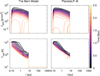 |
Fig. B.1 Comparison of the circumprimary disc evolution for the nominal case with abin = 20 au, between the results obtained in this work and those using the PlanetaLP-B code (Ronco et al. 2021). As in figure 2, the top panels display the evolution of the gas surface density, while the bottom panels show the evolution of the disc midplane temperature. |
Appendix C Disc lifetimes: effect of external photoevaporation
When we analysed the evolution of the S-type gaseous discs in Sect. 3.1, we noted that the disc lifetimes reached a maximum at abin ≈ 50 au for our nominal set-up (see Table 2). In this Appendix we demonstrate that this counter-intuitive effect of having disc lifetimes which do not always decrease with smaller binary separation, is an effect of the external photoevaporation. Indeed, Table C.1 displays the disc lifetimes, with and without external photoevaporation, for a range of binary separations. We note that if external photoevaporation is neglected, the disc lifetimes always decrease with decreasing abin, as expected.
The external photoevaporation considered in this work, which stems from the Bern Model from Emsenhuber et al. (2021a) is that of Matsuyama et al. (2003). The gas removal rate from that simple model is only effective for radial distances r > 18 au, as Fig. C.1 shows. This is why we see no differences in the disc lifetimes between the model with and without external photoevaporation for truncation radius Rtrunc < 18 au (or abin < 50 au) in Table C.1. For discs which are truncated at larger radius than 18 au, external photoevaporation becomes increasingly important in removing gas for larger orbital distances (the more distant the gas is from the primary star, the less bound and easier to remove). This is why disc lifetimes get slightly reduced from abin from 50 au outwards in the nominal setup with external photoevaporation.
![Mathematical equation: $\[\left(\tau_{\text {disc }}^{\prime}\right)\]$](/articles/aa/full_html/2026/04/aa57243-25/aa57243-25-eq26.png)
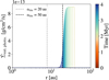 |
Fig. C.1 External photoevaporation rate as a function of time for the model of Matsuyama et al. (2003), applied to the nominal disc with abin = 100 au (disc truncated at Rtrunc = 38.5 au). The 2 extra vertical lines indicate the truncation radius corresponding to a disc with abin = 20 (grey) and abin = 50 au (black). External photoevaporation is negligible for r < 18 au. |
All Tables
All Figures
|
Fig. 1 Disc truncation radius in units of the binary semi-major axis as a function of the binary mass ratio (q) for the circumprimary (violet lines) and circumsecondary discs (orange lines). The solid lines correspond to a binary with ebin = 0, and the dashed lines indicate the case where ebin = 0.5. |
| In the text | |
|
Fig. 2 Evolution of the gas disc as a function of orbital distance from the primary for the nominal disc with binary separations of abin = 20 au (left) and abin = 100 au (right). The grey background curves correspond to the single-star case. The disc profiles are shown every 105 years. The top panels display the evolution of the gas surface density, and the bottom panels show the evolution of the disc midplane temperature. |
| In the text | |
|
Fig. 3 Evolution of the pebble disc as function of orbital distance from the primary for the nominal disc with binary separations of abin = 20 au (left) and abin = 100 au (right). The grey background curves correspond to the single-star case. The disc profiles are shown every 105 years. The top panels indicate the evolution of the pebble surface density, and the bottom panels show the evolution of the pebble sizes. The abrupt change in the pebble size at r ~ 0.4–5 au for all the profiles and times corresponds to the location of the water-ice line. This also affects the profiles of the pebble surface density. |
| In the text | |
|
Fig. 4 In situ planet growth by pebble accretion at ap = 5 au (top panel) and ap = 20 au (bottom panel). The solid lines indicate the evolution of the total planet mass, and the dashed lines show the evolution of the core mass. The different colours correspond to different binary separations, as indicated in the labels. After the final planet mass is reached during the disc lifetime (a few million years), the planet evolves during gigayears by cooling and contraction. |
| In the text | |
|
Fig. 5 Binary mass ratio vs. binary separation (top panel) and binary mass ratio vs. disc truncation radius (bottom panel) for systems that formed a planet at least more massive than Mars. The colour bar indicates the final planet mass. The shaded contour regions represent areas with the highest number planet density, derived from a two-dimensional KDE performed on planets with masses greater than 10 M⊕. The lack of planets for Rtrunc>400 au stems from the choice of the upper limit on abin = 1000 au (see Table 1). |
| In the text | |
|
Fig. 6 Number of formed S-type planets as a function of binary semi-major axis (abin) from the grid of 5000 simulations presented in Sect. 3.4. The dashed black line illustrates the log-uniform distribution of abin adopted as the initial condition (multiplied by 0.5 for better visualisation). The different colours of the bars correspond to different ranges of planet mass, indicated in the legend of the figure. The simulations assumed one embryo per disc and did not include the gravitational perturbation from the secondary or orbital migration. |
| In the text | |
|
Fig. 7 Initial planet location relative to the binary separation, ap,0/abin, vs. final planet mass (top panel) and initial planet location relative to the disc truncation radius, ap,0/Rtrunc, vs. final planet mass (bottom panel) for systems that formed a planet at least more massive than Mars. The colour bar indicates the initial mass of solids in the disc after truncation. The x-axis scale is different in each plot. |
| In the text | |
|
Fig. 8 Same as Figure 3 for the abin = 100 au case (and single-star in the grey background), but taking into account the growth of the giant planet at 5 au and the feedback of it on the disc. The evolution of the planet mass is shown in Fig. 4 for the binary and single-star cases. |
| In the text | |
|
Fig. B.1 Comparison of the circumprimary disc evolution for the nominal case with abin = 20 au, between the results obtained in this work and those using the PlanetaLP-B code (Ronco et al. 2021). As in figure 2, the top panels display the evolution of the gas surface density, while the bottom panels show the evolution of the disc midplane temperature. |
| In the text | |
|
Fig. C.1 External photoevaporation rate as a function of time for the model of Matsuyama et al. (2003), applied to the nominal disc with abin = 100 au (disc truncated at Rtrunc = 38.5 au). The 2 extra vertical lines indicate the truncation radius corresponding to a disc with abin = 20 (grey) and abin = 50 au (black). External photoevaporation is negligible for r < 18 au. |
| In the text | |
Current usage metrics show cumulative count of Article Views (full-text article views including HTML views, PDF and ePub downloads, according to the available data) and Abstracts Views on Vision4Press platform.
Data correspond to usage on the plateform after 2015. The current usage metrics is available 48-96 hours after online publication and is updated daily on week days.
Initial download of the metrics may take a while.