| Issue |
A&A
Volume 708, April 2026
|
|
|---|---|---|
| Article Number | A66 | |
| Number of page(s) | 10 | |
| Section | The Sun and the Heliosphere | |
| DOI | https://doi.org/10.1051/0004-6361/202557284 | |
| Published online | 26 March 2026 | |
Morphological variations of solar granules in the presence of magnetic fields
1
Astronomical Institute of the Czech Academy of Sciences, Ondřejov, Czech Republic
2
Universidad Nacional de Colombia, Observatorio Astronómico Nacional de Colombia, Bogotá, Colombia
3
Institut für Sonnenphysik (KIS), Freiburg, Germany
4
Max-Plank Institute for Solar System Research, Göttingen, Germany
★ Corresponding authors: This email address is being protected from spambots. You need JavaScript enabled to view it.
; This email address is being protected from spambots. You need JavaScript enabled to view it.
Received:
17
September
2025
Accepted:
15
February
2026
Abstract
Context. Solar granulation consists of dynamic convective plasma cells that rise from the solar interior to the surface. The interaction between this plasma cells and the Sun’s magnetic field provides valuable insights into the dynamics of plasma near the solar surface and how it changes in the presence of magnetic field.
Aims. This study aims to analyse the morphological characteristics of solar convective cells, investigating the relationship between magnetic field properties and granule dynamics. In particular, we examine how granule properties, such as area, shape, and brightness, vary under different magnetic field conditions.
Methods. This research used observations of the active region NOAA 11768 taken by the Swedish 1-m Solar Telescope (SST). We applied the segmentation algorithm on the continuum intensity images to identify individual granules and determine their sizes, shapes, and mean brightness. We determined the magnetic field vector and line-of-sight velocity from the CRISP spectropolarimetric data to investigate the role of these parameters on the properties of granules.
Results. We found that granule area decreases systematically with increasing magnetic field strength, with the largest granules found in non-magnetic regions and a mean granule area of approximately 1.58 arcsec2 with an effective diameter of 1.42 arcseconds. Both mean continuum intensity and granule size decrease with stronger magnetic fields, demonstrating the suppression of convective energy transport in magnetised regions. However, we do not find any correlation between the mean brightness of granules and mean up-flow velocity within the granules. We observe highly elongated granules in both magnetic and non-magnetic regions, but close to circular granules are observed only in non-magnetic areas. We find indications of alignment between the major axis of granules and magnetic field azimuth in regions with a strong horizontal component of the magnetic field. These findings confirm that granules are highly sensitive to the presence of magnetic fields, with strong fields inhibiting lateral expansion of convective cells.
Key words: Sun: evolution / Sun: granulation / Sun: magnetic fields / Sun: photosphere
© The Authors 2026
 Open Access article, published by EDP Sciences, under the terms of the Creative Commons Attribution License (https://creativecommons.org/licenses/by/4.0), which permits unrestricted use, distribution, and reproduction in any medium, provided the original work is properly cited.
This article is published in open access under the Subscribe to Open model. This email address is being protected from spambots. You need JavaScript enabled to view it. to support open access publication.
1. Introduction
Solar granulation is a manifestation of the subsurface convection in the solar photosphere, which presents itself as a pattern of bright cellular elements surrounded by darker intergranular lanes. These structures are important to understand solar surface dynamics, and they have been extensively studied through both observational and numerical approaches (i.e. Roudier & Muller 1986; Müller 1989; Hirzberger et al. 1997; Danilovic et al. 2008). The larger part of the solar surface exhibits this granulation pattern, where convective cells heat the photosphere with the hot material rising from the upper layer of the convective zone. The emerged small-scale magnetic field is dragged by such convective cells (Cheung & Isobe 2014; Guglielmino et al. 2020). While no singular characteristic size exists for granular cells, studies consistently report a mean diameter between 1″ and 2″ (approximately 725–1450 km) in quiet-Sun regions (Wöhl & Nordlund 1985).
Earlier studies reported varying characteristic sizes from 1.1″ (Namba & Diemel 1969) to 1.35″ (Bray & Loughhead 1984) and mean intergranular distances of 1.76″ (Roudier & Muller 1986). These granules may in turn grow and fragment, merge with others, or shrink and decompose (Bahng & Schwarzschild 1961; Title et al. 1986; Mehltretter 1978). However, more recent investigations have revealed a distinct population of smaller convective cells with spatial scales below 600 km (e.g. Roudier et al. 2003; Yu et al. 2011), as identified both observationally and in high-resolution solar radiation hydrodynamics simulations (Stein et al. 2009; Abramenko et al. 2012; Rempel 2014).
The properties of granulation in regions of strong magnetic field exhibit additional complexity due to the interaction between such field and the convective plasma. From a quantitative point of view, studies of such interactions, similar to those performed by Aparna et al. (2025), demonstrate that stronger vertical fields increasingly suppress horizontal surface motions, suggesting morphological variations in the granulation in regions of magnetic flux emergence. In the case of sunspot umbrae, magneto-convection manifests as umbral dots (Sobotka & Puschmann 2009), while in penumbrae, where magnetic fields are weaker and more inclined, convective cells become highly elongated, forming characteristic filaments (Rempel 2011; Tiwari et al. 2013). Moreover, granules in plage regions typically exhibit reduced sizes and lower line-of-sight (LOS) velocities compared to field-free granulation (Narayan & Scharmer 2010). Also, broad light bridges in sunspots show a granular pattern where the properties of convective cells are comparable to the quiet-Sun granules (Lagg et al. 2014); however, they are smaller and have longer lifetimes (Hirzberger et al. 2002). Early observations indicate that the sizes of granules are smaller than average near sunspots (Schröter 1964; Macris 1979), while granules can be highly elongated in regions of flux emergence (Schlichenmaier et al. 2010; Centeno et al. 2007). Previous studies have indicated a characteristic scale diameter of approximately 1.37″ that distinguishes different granular behaviours, suggesting a transition between turbulent eddies and convective elements (Roudier & Muller 1986).
The objective characterisation of the fine-structure in solar granulation requires robust pattern recognition algorithms. However, the absence of a priori criteria for physically meaningful structures has led to various methodological approaches, each producing systematically different patterns.
Traditional techniques employ Fourier-based recognition with single-level intensity thresholds. This approach has inherent limitations in structure separation (i.e. Roudier & Muller 1986; Title et al. 1989; Hirzberger et al. 1997; Berrilli et al. 2005; Bovelet & Wiehr 2007; Yu et al. 2011). More sophisticated methods applying machine-learning techniques have been developed to address these constraints (e.g. Feng et al. 2013; Chola & Benifa 2022; Díaz Castillo et al. 2022), yet challenges remain in balancing pattern recognition accuracy with physical relevance.
The interaction between the magnetic field and plasma convective cells is a crucial aspect of solar surface dynamics, in particular, at granular scales. Using high-resolution observations, multiple studies have shown that horizontal motions inside granules carry vertical magnetic flux towards the intergranular lanes (Harvey et al. 2007; Centeno et al. 2007). The emergence of the magnetic field can disturb the granulation patterns and shapes, leading to the appearance of dark lanes or so-called abnormal granulation (Cheung et al. 2007). The statistical approach to understanding granulation patterns and their relationship with magnetic fields remains relatively unexplored. This presents an opportunity for a systematic investigation using high-resolution observational data from modern large solar telescopes and new techniques. Note that rudimentary analysis of the data was already performed by Jurčák et al. (2017), but the present analysis is more thorough and implements more advanced procedures for the segmentation and characterisation of the identified convective cells.
2. Observations and data processing
The analysis of the active region NOAA 11768 was performed using observations obtained from the 1-m Swedish Solar Telescope (SST; Scharmer et al. 2003). The instruments on the SST provide full spectropolarimetric data for studying solar magnetic features at high spatial resolutions as well as continuum intensity images. We analysed data from June 13, 2013, capturing a rudimentary sunspot, a number of pores, and flux emergence regions within the field of view (FOV). The active region emerged on the solar surface on June 11, 2013, and grew during the observation period; see Fig. 1.
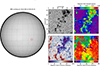 |
Fig. 1. Left: Full-disk image context from the Helioseismic and Magnetic Imager (HMI) on board the Solar Dynamics Observatory (SDO). The red rectangle shows the region of interest observed by the 1-m SST. Right: Four-image grid displaying maps obtained from the SST data, including (a) blue-continuum intensity image, (b) strength of the magnetic field, (c) magnetic field inclination, and (d) magnetic field azimuth. |
The observational data comprise two main datasets. First, the blue-continuum images were processed using the multi-object multi-frame blind deconvolution (MOMFBD) technique (Van Noort et al. 2005), achieving a temporal cadence of 5.6 s and a spatial sampling of 0.034 arcsec pixel−1 (see Fig. 1.a). These observations were recorded between 8:21 UT and 10:50 UT. Second, the CRisp Imaging SpectroPolarimeter (CRISP) instrument (Scharmer et al. 2008) collected full Stokes vector profiles of the Fe I 525 nm line with a temporal cadence of 31 s and a spatial sampling of 0.058 arcsec pixel−1 (see measurements by Norén 2013) between 8:36 UT and 10:54 UT. The imaging and CRISP data were carefully co-aligned to ensure precise spatial correspondence.
2.1. Inversion of the CRISP data
To determine the magnetic field properties, we used the Very Fast Inversion of the Stokes Vector (VFISV) code by Borrero et al. (2011) to perform Milne-Eddington inversions of the Stokes vector profiles, obtaining magnetic field strength (Fig. 1.b), inclination (Fig. 1.c), and azimuth (Fig. 1.d). The 180° ambiguity in the magnetic field azimuth problem was solved using the AMBIG code (Leka et al. 2009), followed by the transformation of the magnetic field inclination and azimuth from the LOS to the local-reference frame using the AZAM routines written by Paul Seagraves at the High Altitude Observatory (described in Lites et al. 1995).
We also used the retrieved LOS velocity values in our analysis (not shown in Fig. 1). The LOS velocities were corrected for convective blueshift in two steps. First, we computed the average LOS velocity in the quiet-Sun regions and subtracted this value from the entire velocity map. This procedure removes velocity contributions arising from the Earth’s orbital motion and solar rotation, yielding a zero mean LOS velocity in the quiet-Sun. Second, we applied a correction for convective blueshift, based on the measurements and calculations of Löhner-Böttcher et al. (2019) who quantified the convective blueshift of the Fe I 525 nm line. Accounting for the spectral resolution of CRISP and the μ angle of the observed region, we applied a uniform velocity offset of −0.33 km s−1. Although this correction is tentative, it yields reasonable mean up-flow velocities in the segmented granules.
In the analysed dataset, the signal-to-noise level was around 200 for the Stokes profiles of the polarised light. An intrinsic limitation of inversion codes is their tendency to fit noise. Therefore, even in the quiet areas of the FOV, we obtain a non-zero magnetic field vector. Based on the inversion results in the most quiet regions of the FOV, the magnetic field strength has a mean value of 75 G, with a standard deviation of 26 G. As the Stokes Q and U profiles are proportional to B2 and Stokes V is proportional to B, we obtain magnetic field inclination in the LOS frame around 90° in the quiet areas where signals are dominated by noise.
2.2. Segmentation
The data preparation involved scaling and co-aligning the blue-continuum observations with respect to the CRISP dataset to ensure accurate spatial correspondence. Therefore, the spatial sampling of the blue-continuum images was downscaled to match the spatial sampling of CRISP data. Since our work focuses on the regions of the quiet-Sun and the emergence of magnetic field, we masked the active region in the analysed region of interest. The initial threshold was set to 50% of the intensity I/IQS, and the subsequent performance of the segmentation algorithm improved the masking of the remaining penumbral regions, as these features show much lower intensity values than solar granulation.
Our granulation segmentation algorithm involved multi-step image processing to achieve an accurate identification of granules, similar to the Multi-Level Thresholding (MLT4) algorithm proposed by Bovelet & Wiehr (2007). In the initial step (Fig. 2.a), a small region of 250 × 250 pixels (∼14 × 14 arcseconds) was extracted from the processed blue continuum intensity images. Subsequently (Fig. 2.b), local minima detection and watershed segmentation were applied to generate a segmented map with preliminary granule identification. By leveraging most of the MLT4 features, we refined the segmentation process by strategically modifying the segmentation parameters. The algorithm enables selective contour preservation, where white line segments are retained while black line segments are eliminated (see Fig. 2.c). This selective filtering enhances the initial segmentation accuracy.
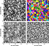 |
Fig. 2. Segmentation process of solar photospheric granules. (a) Original solar surface region. (b) Initial granule segmentation using local minima and the watershed technique. (c) Refined contour selection after parameter optimisation. (d) Final granule morphology after contour-based erosion. |
The final step (Fig. 2.d) implemented a contour-based erosion approach, refining granule boundaries derived from the optimised segmentation map. White granules or segments represent structures that were split into new segments from the initial segmentation, while bright lines within segments indicate regions that were merged into one segment compared to the initial segmentation1.
For each segment, we calculated the area, eccentricity, and orientation. We also determined the mean intensity value of the blue-continuum, the mean strength of the magnetic field (Bstrength), the mean vertical magnetic field (Bvertical), the mean horizontal magnetic field (Bhorizontal), the mean LOS velocity, and the circular average of the magnetic field azimuth (Eq. 2.2.4 Mardia & Jupp 1999). Finally, we cleaned the dataset by removing outliers related to the area of the segments and any entries containing “not a number” (NaN) values. The outliers were removed using standard score or z-score (Kreyszig 1979), where values with |zscore(areas)| > 3 are considered outliers. To retain more data points from the other parameters, we set the outlier threshold to twice the z-score limit (∼13.5 arcsec2).
2.3. Eccentricity and orientation
Using standard libraries (i.e. scikit-image van der Walt et al. 2014), we computed most of the morphological properties, including eccentricity. The initial standard method used for eccentricity calculation depends on the length of the major and minor axes. These are derived from the second central moments of each region by fitting the best ellipse to each segment. Since solar granular patterns do not have perfect circular or elliptical shapes, this method for the calculation of the eccentricity could present certain issues. In addition, the fact that segmentation eventually fails to extract granules properly renders these calculations difficult.
Hence, we introduced two custom approaches to determine the eccentricity of granules. The first approach consists of three steps. First, we computed the geometrical centroid of the region or segment, defined as a point within the granule most distant from its boundary. This was calculated ‘by replacing each foreground (non-zero) element with its shortest distance to the background (any zero-valued element)’2 rather than using the geometrical shape itself, to avoid centroids outside the segments. Then, we calculated the line connecting the two most distant points passing simultaneously through the centroid, namely the major axis. Finally, we calculated the line perpendicular to the major axis through the centroid, namely the minor axis. For the second approach, we first applied a convex hull transformation (see Chapter 11; Berg et al. 2010) to each segment and repeated the previous steps. In Appendix A we describe and show the differences between each eccentricity calculation approach.
As the final data product, we computed the angular difference between the orientation of each granule’s major axis obtained from the previous calculations and its circularly averaged magnetic field azimuth. Since we considered the relative difference between these variables, we calculated the angular difference within a range of 0° (when the magnetic field azimuth and the major axis are parallel) to 90° (when they are perpendicular). We implemented and adapted all computational procedures and data analysis using custom Python scripts, incorporating the specialised solar physics package Sunpy (Mumford et al. 2023) for enhanced functionality.
3. Results
Figure 3 (top panel) presents the area distribution of all identified granules. The temporal evolution of individual granules is not tracked; consequently, each granule may be counted multiple times throughout its lifespan. The resulting probability density distribution (PDF) follows a negative exponential distribution where the lower limit of the granule sizes is set manually to ∼0.28 arcsec2, which also corresponds to the modal area of the whole dataset. To fit the PDF, we applied a natural logarithm to the PDF and used a standard linear regression to recover the parameters that fit the exponential distribution. This exponential fit to our sample is valid for granules with sizes up to 10 arcsec2, i.e. it fits 99.5% of the 725 044 identified granules. The statistical sample is insufficient for larger granules, counting 3453 cases; thus, we can no longer claim that the power law is valid for segmented areas larger than 10 arcsec2. To fit the exponential distribution, we linearised it in the form
 (1)
(1)
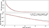 |
Fig. 3. Granule area distributions. Top panel: Raw distribution of granule areas including outliers, with a fixed bin width of ∼0.15 arcsec2. Bottom panel: Histogram log(PDF) vs area, where the PDF is the normalised probability density of the area distribution. The dashed red line represents the fitting of the distribution to the derived parameters. |
where PDFarea is the PDF of the granule areas, A is the amplitude or scaling factor adjusting the height of the distribution (A is expected to be ∼1/β), and the parameter β (area units) is the mean (expected value) of the distribution (see Balakrishnan & Basu 1996, for more details on the exponential distribution). From fitting the right side of Eq. (1) (bottom panel in Fig. 3), we find that the mean area is ∼1.58 arcsec2 or an effective diameter of ∼1.42 arcseconds, close to d = 1.31 arcseconds reported by Roudier & Muller (1986).
To better illustrate the importance of the eccentricity approaches described in Sect. 2.3 and Appendix A, we present two-dimensional kernel density estimation (2D KDE) plots of granule areas versus eccentricities calculated using the three methods. We use a grid size (number of bins) and number of levels of 100, which corresponds to a bin width of approximately half the lower granule-area limit mentioned previously (∼0.14 arcsec2). To highlight regions of the KDE with significantly lower population than the maximum, we applied the logarithm to the distribution, as illustrated in Fig. 3. Each KDE plot evaluates the joint distribution between the areas of the segments and the eccentricity measurements. This approach identifies patterns in the most common area and eccentricity values as well as their statistical relationship across the entire granule population.
Figure 4 displays the 2D KDE plots of the three different eccentricity approaches, with the log-transformed kernel density, log(KDE). The left panel uses raw eccentricity – defined by the best-fitting ellipse derived from segment moments – shows a high concentration of granules with eccentricities between 0.84 and 0.91. Under this metric, it indicates that most granules appear highly elongated. Additionally, the plot shows a lower probability eccentricity boundary near 0.1, with virtually no granules measured below this threshold.
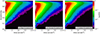 |
Fig. 4. 2D-log(KDE) plots showing the distribution of the areas and the three eccentricity metrics: (a) raw eccentricity (ellipse fitting), (b) convex eccentricity (computed on convex hulls), and (c) custom eccentricity (based on extreme points through the centre of mass of the segments). Each plot highlights the most probable eccentricity-area combinations and reveals trends. |
The centre panel in Fig. 4 reveals maximum density probabilities for eccentricities from 0.72 to 0.82. This shift towards lower eccentricity values implies that the approach based on convex-hull eccentricity detects less elongated, more geometrically natural granule shapes. It also reveals more ‘circular’ granules, since the plot shows density contours in lower eccentricity values close to zero. Although this behaviour may indicate a more responsive eccentricity measure, it is important to note that the convex hull transformation can sometimes introduce distortions in the granule shape representation (see Test segment 4 in Fig. A.1).
Using custom eccentricity, the third KDE plot (Fig. 4, right panel) illustrates a behaviour similar to the convex hull approach with a realistic representation. The highest density region observed ranges with values between 0.72 to 0.83 but includes local maximum around ∼0.63. This is higher than convex eccentricity but more sensitive to moderately elongated granular structures. This method also permits eccentricity values approaching zero (circular shapes), offering a broader and more continuous range of morphological representations. Furthermore, the trend between areas and eccentricities shows that larger granules exhibit higher eccentricities, since the most likely eccentricity for granules with areas greater than 3.5 arcsec2 is around 0.9, larger than for smaller granules.
The KDE colour scale is normalised and reflects the statistical spread of the data: black indicates probabilities of 10−3 or lower, while light-grey indicates a probability of 1 and therefore high concentration in the combined data. Hereafter, the term ‘eccentricity’ denotes custom eccentricity. Appendix A describes in detail the motivation behind this approach.
The 2D-KDE plots in Fig. 5 provide insight into several relationships between granular morphological properties and physical conditions. Table 1 summarises the maximum probability values in each KDE plot. The colour-coding in Fig. 5 follows the same convention as Fig. 4, enabling consistent interpretation across figures.
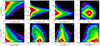 |
Fig. 5. 2D-log(KDE) plots showing the dependence of: (a) granule area on granule eccentricity, (b) granule area on granule continuum intensity, (c) granule area on granule LOS velocity, and (d) granular continuum intensity on granule LOS velocity. Bottom: Dependence of granule (e) area, (f) continuum intensity, (g) LOS velocity, and (h) eccentricity on magnetic field strength. The colour-coding follows the same scheme, as in Fig. 4. |
Maximum probability values determined by each 2D KDE.
Panel (a) in Fig. 5 replicates panel (c) in Fig. 4. The highest density region occurs near an eccentricity of ∼0.77 and an area value of ∼0.55 arcsec2. Larger granules appear more elongated.
Panel (b) in Fig. 5 shows the correlation between the granule area and the continuum intensity. The maximum likelihood of granular brightness is independent of the size of the granules; it is ∼1.03 I/IQS. However, as granules increase in size, we observe less scatter in their mean brightness (noting that this trend is primarily caused by the lower number of large granules). We note that the population of small and darker granules can be identified in the PDF as an extended red region for very small granules.
In panel (c) of Fig. 5, we examine the relationship between granule areas and LOS velocities. The resulting KDE is comparable to panel (b). We find that the maximum likelihood of the LOS velocity is around −0.4 km s−1 for granules of all sizes. As in panel (b), smaller granules have a higher spread in the mean LOS velocity; however, again, this trend is primarily caused by the lower number of large granules.
Panel (d) in Fig. 5 illustrates the relationship between granule continuum intensity and LOS velocity, revealing a symmetric structure centred at I/IQS ≈ 1.08 and vLOS ≈ −0.5 kms−1. This 2D-KDE illustrates that mean brightness of granules does not obviously correlate with their mean LOS velocity, i.e. stronger up-flows in granules do not result in brighter granules. This does not contradict the intuitive expectation that the brightest parts of the granules have the strongest up-flows (as shown for penumbral filaments by Tiwari et al. 2013). Indeed, we must keep in mind that we are averaging both the brightness and the LOS velocity over the whole area of the segmented granule. We conclude that this averaging process eliminates dependence between these parameters.
In panel (e) of Fig. 5, we show the 2D-KDE between granules area and magnetic field strength. The most frequent B found in the FOV is around 205 G and can be partially attributed to the noise level in the data, as discussed in Sect. 2.1. We observe that granule area decreases with increasing magnetic field strength. The largest granules are found in non-magnetic regions, while higher magnetic strengths are associated with significantly smaller convective cells. This suggests that magnetic fields inhibit the lateral expansion of granules. We observe no signature of equipartitional magnetic field strength (Beq ∼ 600 G in the photosphere) in the KDE plots – neither in panel (e) nor in panels (f), (g), or (h) discussed later.
Panel (f) in Fig. 5 shows the relationship between continuum intensity and magnetic field strength. The peak density occurs around I/IQS ∼ 1.07 and B ∼ 185 G. The KDE naturally captures fluctuations around the dominant trend, while the ridge of maximum probability density traces the most representative physical behaviour. As magnetic field strength increases, the continuum intensity decreases, providing evidence that strong magnetic fields suppress convective energy transport within these regions.
Panel (g) illustrates the relationship between magnetic field strength and LOS velocity. The distribution centres on up-flows (vLOS ≈ −0.56 km/s). With increasing field strength, the distribution of LOS velocities narrows, but this is partially caused by the lower number of granules with high values of B. The KDE also shows that granules in regions with a weak magnetic field have an asymmetric distribution with preference for stronger up-flows. However, this asymmetry disappears for granules located in regions with a stronger magnetic field.
Panel (h) in Fig. 5 illustrates the magnetic field strength influence on the granule eccentricity. This plot reveals that high eccentricities dominate across the entire range of magnetic field strengths, with the highest probability density consistently concentrates at eccentricity values ≈0.85. The plot shows that lower magnetic field strengths allows more circular granule shapes.
The 2D-KDE plots in Figs. 6, 7, 8 show details of the granular morphological properties and their relationship to different horizontal magnetic field regimes. Figure 6 illustrates the dependence of granule areas on eccentricity, influenced by the horizontal component of the magnetic field. Panel (a) corresponds to the 0–300 G range, which represents approximately 58% of the data in the analysed FOV and closely resembles the global distribution shown previously in panel (c) of Fig. 4. This magnetic regime is typically associated with quiet-Sun regions. As we advance through panels (b-f), we observe a progressive evolution in the area-eccentricity relationship.
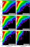 |
Fig. 6. 2D-KDE plots showing the dependence of area on eccentricity, segmented by horizontal magnetic field (Bhorizontal). Panel (a): 0–300 G,(∼58% of detected granules). Panels (b)-(f): Area-eccentricity relationship across different horizontal magnetic field ranges. The colour-coding follows that in Fig. 4. |
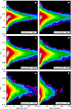 |
Fig. 7. 2D-KDE plots illustrating the relationship between granule area and continuum intensity, and their dependence on the horizontal magnetic field. Panel (a) represents the 0–300 G range. Panels (b)-(f) show the evolution of the area-intensity relationship across other horizontal magnetic field ranges. The colour-coding follows that in Fig. 4. |
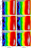 |
Fig. 8. 2D-KDE plots showing the relationship between granule area and Δθ, as influenced by the horizontal magnetic field. Panel (a) covers 0–300 G. Panels (b)-(f) illustrate how the area–Δθ relationship evolves across different horizontal magnetic field ranges. The colour-coding follows that in Fig. 4. |
In regions of weak horizontal magnetic field, the distributions appear broad, and the highest probability densities favour larger granules. As the horizontal magnetic field strength increases, the distributions shrink, with high-probability regions shifting towards smaller granule areas. This is in agreement with panel (e) of Fig. 5. Additional information provided in Fig. 6 shows the distribution of eccentricity based on the horizontal magnetic field strength. While the maximum likelihood of granule eccentricity does not depend on Bhor, the granule areas begin to be truncated as Bhor increases, thereby strongly shrinking the shape of the distribution. This shows that for strong magnetic fields, the density of large and elongated granules decreases whilst small granules are more likely to appear, a behaviour which is not evident from panel (h) of Fig. 5.
Figure 7 explores the relation between the granule area and the continuum intensity across varying horizontal magnetic field strengths. Panel (a) corresponds to the 0–300 G range and closely resembles the full distribution presented in Fig. 5(b). Moreover, Fig. 7 provides additional information than Fig. 5(b), as includes the KDE shown in Figs. 5(e) and (f).
As the horizontal magnetic field increases across panels (b)-(f), systematic changes occur in the KDEs. The analysis reveals that the ‘tails’ of the 2D KDE distribution shift progressively downwards with increasing horizontal magnetic field strengths, i.e. we do not observe large granules in regions of strong magnetic field, as indicated in Fig. 5(e). We also see that the most common intensity of the granules decreases with increasing field strengths, as indicated in Fig. 5(f). On the other hand, the probability of dark granules with ∼0.8 I/IQS is almost independent of the horizontal magnetic field; in regions with Bhorizontal > 600 G, it slightly increases. Also, bright granules are observed in regions with strong magnetic fields, although less frequently than in quiet-Sun regions. This behaviour highlights the progressive suppression of both granule expansion and brightness as magnetic field strength increases, demonstrating the inhibitory effect of strong magnetic fields on convective processes within solar granulation.
Figure 8 examines the relationship between granular eccentricity and the angular difference Δθ in different horizontal magnetic field regimes, where Δθ is explained in Sect. 2.3. We note that values closer to 0° suggest that the horizontal magnetic field affects the morphology parameters of the granules.
Panel (a) corresponds to regions with horizontal magnetic fields ranging from 0–300 G, characteristic of quiet-Sun regions. The distribution appears uniform along Δθ, indicating that granules of all eccentricities span the full range from parallel to perpendicular orientations. This suggests weak coupling between granule orientation and magnetic field azimuth at small horizontal magnetic field strengths. The same behaviour is also observed for granules located in regions with Bhorizontal between 300 G and 400 G. For stronger Bhorizontal, we find that the maximum likelihood of highly eccentric granules (≈0.9) is localised between Δθ = 10° and 20°, suggesting that the magnetic field is aligned with the major axis of the granule in these magnetic regimes. For the strongest horizontal fields (panels e and f, Bhorizontal > 600 G), the alignment becomes less strong, likely reflecting the reduced number of granules observed within these intervals. We note that apart from the location and shape of the maximum likelihood (white-grey in the KDEs), the KDEs do not depend on the Bhorizontal.
4. Discussion and conclusions
We conducted a statistical study of convective cell properties in the presence of magnetic fields. The analysis comprises the full range of granulation patterns observed in the SST FOV – from quiet-Sun regions, through flux emergence, to a close pore and sunspot neighbourhood. The findings corroborate and expand on previous case studies that examined convection under magnetic influence. For example, realistic 3D magneto-convection simulations demonstrate that strong magnetic fields concentrate into segmented structures and micropores along intergranular lanes, suppressing up-flows and altering convective cell structure and dynamics from field-free cases (Vögler et al. 2005).
Regarding granular sizes, we measure a mean granule area of approximately 1.58 arcsec2 with an effective diameter of 1.42 arcseconds, consistent with the diameter of 1.31 arcseconds reported by Roudier & Muller (1986). Concerning the relationship between granular morphology and magnetic field conditions, we confirm that granules are highly sensitive to the magnetic field. Our analysis demonstrates that granule area decreases systematically with increasing magnetic field strength. The largest granules are predominantly found in non-magnetic regions, while higher magnetic field strengths are associated with significantly smaller convective cells, indicating that relatively strong magnetic fields inhibit the lateral expansion of granules.
Both the mean continuum intensity of the granules and their size decrease systematically with increasing magnetic field strength, as shown in panels (e) and (f) of Fig. 5 and in Fig. 7. This demonstrates the suppression of convective energy transport in magnetised regions, where stronger fields result in both smaller and dimmer granular structures.
Morphological analysis reveals that maximum granule eccentricity increases with the horizontal magnetic field strength, as shown in Fig. 6. The probability of finding perpendicular alignment between the granule orientation and the magnetic field azimuth (Δθ approaching 90°) decreases significantly as the horizontal field strength increases (Fig. 8). This alignment effect is particularly prominent in flux emergence regions, where highly elongated granules connect opposite polarity regions. These morphological changes manifest the fundamental sensitivity of convective cells to magnetic field properties, as magnetic fields can significantly modify granule shapes and orientations.
Line-of-sight velocity analysis demonstrates that the majority of granules exhibit up-flows, with the distribution centred around −0.4 km s−1. We also investigated in detail the role of the magnetic field on the LOS velocity. It turns out that the trend in panel (g) of Fig. 5 – smaller velocity span with increasing |B| – is caused by the lower number of granules in regions in strong |B| regions. We obtain comparable LOS velocity distributions for regions with different magnetic field strength (not displayed in any figure). We also want to stress that our statistical study shows that the mean granule brightness does not correlate with the mean granule LOS velocity, i.e. stronger up-flows in granules do not result in brighter granules. We want to stress that this finding does not contradict the intuitive expectation that the brightest parts of granules have the strongest up-flows, as we compare average values over the whole granule area.
These findings demonstrate the mutual interaction between convective cells and magnetic fields. While magnetic fields suppress granular convection and modify granule morphology, the convective motions can also influence magnetic field configurations through processes such as LOS field advection and magnetic flux concentration between granular boundaries.
Future work will incorporate temporal evolution by applying a tracking algorithm to the segmented granules to investigate the dependence of convective cell lifetime on magnetic field strength and to analyse the evolution of magnetic field properties throughout individual granule lifespans. Such an approach will extend the present statistical analysis to a Lagrangian description of magneto-convection and allow us to directly link morphological changes to the temporal evolution of the magnetic field (e.g. Zhang et al. 2009). In addition, the inclusion of apparent horizontal granular motions and their dependence on magnetic field will be particularly relevant. Previous studies indicate that such flows are important for plasma–magnetic field coupling and may have implications for energy transport into the upper solar atmosphere (see Welsch 2015; Tilipman et al. 2023), whereas stronger magnetic fields tend to suppress horizontal motions (e.g. Title et al. 1992; Aparna et al. 2025). Examining how granular flows and morphology vary across different magnetic environments will further help constrain coupling between convection and magnetic fields in the quiet-Sun.
Acknowledgments
This research is supported by the Czech–German common grant, funded by the Czech Science Foundation under the project 23-07633K and by the Deutsche Forschungsgemeinschaft under the project BE 5771/3-1 (eBer-23 13412) and the institutional support RVO:67985815. This research has made use of NASA’s Astrophysics Data System Bibliographic Services. The research was sponsored by the DynaSun project and has thus received funding under the Horizon Europe programme of the European Union under grant agreement (no. 101131534). Views and opinions expressed are however those of the author(s) only and do not necessarily reflect those of the European Union and therefore the European Union cannot be held responsible for them.
References
- Abramenko, V. I., Yurchyshyn, V. B., Goode, P. R., Kitiashvili, I. N., & Kosovichev, A. G. 2012, ApJ, 756, L27 [NASA ADS] [CrossRef] [Google Scholar]
- Aparna, V., Tiwari, S. K., Moore, R. L., et al. 2025, ApJ, 987, 98 [Google Scholar]
- Bahng, J., & Schwarzschild, M. 1961, ApJ, 134, 312 [NASA ADS] [CrossRef] [Google Scholar]
- Balakrishnan, N., & Basu, A. P. 1996, The Exponential Distribution: Theory, Methods and Applications (CRC Press) [Google Scholar]
- Berg, M., Cheong, O., Kreveld, M. O., 2010, Computational Geometry: Algorithms and Applications (Heidelberg: Springer, Berlin) [Google Scholar]
- Berrilli, F., Moro, D. D., Florio, A., & Santillo, L. 2005, Sol. Phys., 228, 81 [CrossRef] [Google Scholar]
- Borrero, J. M., Tomczyk, S., Kubo, M., et al. 2011, Sol. Phys., 273, 267 [Google Scholar]
- Bovelet, B., & Wiehr, E. 2007, Sol. Phys., 243, 121 [Google Scholar]
- Bray, R. J., & Loughhead, R. E. 1984, Science, 226, 571 [NASA ADS] [Google Scholar]
- Centeno, R., Socas-Navarro, H., Lites, B., et al. 2007, ApJ, 666, L137 [CrossRef] [Google Scholar]
- Chetverikov, D., & Khenokh, Y. 1999, in Computer Analysis of Images and Patterns, eds. F. Solina, & A. Leonardis (Berlin, Heidelberg: Springer, Berlin Heidelberg), 367 [Google Scholar]
- Cheung, M. C. M., & Isobe, H. 2014, Liv. Rev. Sol. Phys., 11, 3 [Google Scholar]
- Cheung, M. C. M., Schüssler, M., & Moreno-Insertis, F. 2007, A&A, 467, 703 [CrossRef] [EDP Sciences] [Google Scholar]
- Chola, C., & Benifa, J. V. B. 2022, Global Trans. Proc., 3, 177 [Google Scholar]
- Danilovic, S., Gandorfer, A., Lagg, A., et al. 2008, A&A, 484, L17 [NASA ADS] [CrossRef] [EDP Sciences] [Google Scholar]
- Díaz Castillo, S. M., Asensio Ramos, A., Fischer, C. E., & Berdyugina, S. V. 2022, Front. Astron. Space Sci., 9, 896632 [Google Scholar]
- Feng, S., Xu, Z., Deng, L., Yang, Y., & Ji, K. 2013, in 2013 6th International Conference on Intelligent Networks and Intelligent Systems (ICINIS), 300 [Google Scholar]
- Guglielmino, S. L., Martínez Pillet, V., Ruiz Cobo, B., et al. 2020, ApJ, 896, 62 [NASA ADS] [CrossRef] [Google Scholar]
- Harvey, J. W., Branston, D., Henney, C. J., Keller, C. U., & SOLIS and GONG Teams, 2007, ApJ, 659, L177 [Google Scholar]
- Hirzberger, J., Vázquez, M., Bonet, J. A., Hanslmeier, A., & Sobotka, M. 1997, ApJ, 480, 406 [NASA ADS] [CrossRef] [Google Scholar]
- Hirzberger, J., Bonet, J. A., Sobotka, M., Vázquez, M., & Hanslmeier, A. 2002, A&A, 383, 275 [EDP Sciences] [Google Scholar]
- Jurčák, J., Lemmerer, B., & van Noort, M. 2017, in Fine Structure and Dynamics of the Solar Atmosphere, eds. S. Vargas Domínguez, A. G. Kosovichev, P. Antolin, & L. Harra, IAU Symp., 327, 34 [Google Scholar]
- Kreyszig, E. 1979, Advanced Engineering Mathematics: Maple Computer Guide, 2nd edn. (U.S.A: John Wiley& Sons, Inc.), 880 [Google Scholar]
- Lagg, A., Solanki, S. K., van Noort, M., & Danilovic, S. 2014, A&A, 568, A60 [NASA ADS] [CrossRef] [EDP Sciences] [Google Scholar]
- Leka, K. D., Barnes, G., Crouch, A. D., et al. 2009, Sol. Phys., 260, 83 [Google Scholar]
- Lites, B. W., Low, B. C., Martinez Pillet, V., et al. 1995, ApJ, 446, 877 [Google Scholar]
- Löhner-Böttcher, J., Schmidt, W., Schlichenmaier, R., Steinmetz, T., & Holzwarth, R. 2019, A&A, 624, A57 [Google Scholar]
- Macris, C. J. 1979, A&A, 78, 186 [Google Scholar]
- Mardia, K., & Jupp, P. 1999, Directional Statistics (Wiley Series in Probability and Statistics) [Google Scholar]
- Mehltretter, J. P. 1978, A&A, 62, 311 [NASA ADS] [Google Scholar]
- Müller, R. 1989, in Solar and Stellar Granulation, eds. R. J. Rutten, & G. Severino, NATO ASI Ser. C, 263, 101 [Google Scholar]
- Mumford, S. J., Freij, N., Stansby, D., et al. 2023, https://doi.org/10.5281/zenodo.8037332 [Google Scholar]
- Namba, O., & Diemel, W. E. 1969, Sol. Phys., 7, 167 [NASA ADS] [CrossRef] [Google Scholar]
- Narayan, G., & Scharmer, G. B. 2010, A&A, 524, A3 [NASA ADS] [CrossRef] [EDP Sciences] [Google Scholar]
- Norén, A. 2013, arXiv e-prints [arXiv:1311.5148] [Google Scholar]
- Rempel, M. 2011, ApJ, 729, 5 [Google Scholar]
- Rempel, M. 2014, ApJ, 789, 132 [Google Scholar]
- Rosin, P. L. 2005, Computing Global Shape Measures (World Scientific), 177 [Google Scholar]
- Roudier, T., & Muller, R. 1986, Sol. Phys., 107, 11 [NASA ADS] [CrossRef] [Google Scholar]
- Roudier, T., Lignières, F., Rieutord, M., Brandt, P. N., & Malherbe, J. M. 2003, A&A, 409, 299 [NASA ADS] [CrossRef] [EDP Sciences] [Google Scholar]
- Scharmer, G. B., Bjelksjo, K., Korhonen, T. K., Lindberg, B., & Petterson, B. 2003, in Innovative Telescopes and Instrumentation for Solar Astrophysics, eds. S. L. Keil, & S. V. Avakyan, SPIE Conf. Ser., 4853, 341 [NASA ADS] [CrossRef] [Google Scholar]
- Scharmer, G. B., Narayan, G., Hillberg, T., et al. 2008, ApJ, 689, L69 [Google Scholar]
- Schlichenmaier, R., Bello González, N., Rezaei, R., & Waldmann, T. A. 2010, Astron. Nachr., 331, 563 [NASA ADS] [CrossRef] [Google Scholar]
- Schröter, E. H. 1964, Atti del Convegno Sulle Macchie Solari, 190 [Google Scholar]
- Sobotka, M., & Puschmann, K. G. 2009, A&A, 504, 575 [NASA ADS] [CrossRef] [EDP Sciences] [Google Scholar]
- Stein, R. F., Lagerfjard, A., Nordlund, A., Geogobiani, D., & Benson, D. 2009, AGU Fall Meeting Abstracts, 2009, SH11B-05 [Google Scholar]
- Taha, A. A., & Hanbury, A. 2015, IEEE Trans. Pattern. Anal. Mach. Intell., 37, 2153 [Google Scholar]
- Tilipman, D., Kazachenko, M., Tremblay, B., et al. 2023, ApJ, 956, 83 [Google Scholar]
- Title, A. M., Tarbell, T. D., Acton, L., Duncan, D., & Simon, G. W. 1986, Adv. Space Res., 6, 253 [Google Scholar]
- Title, A. M., Tarbell, T. D., Topka, K. P., et al. 1989, ApJ, 336, 475 [NASA ADS] [CrossRef] [Google Scholar]
- Title, A. M., Topka, K. P., Tarbell, T. D., et al. 1992, ApJ, 393, 782 [NASA ADS] [CrossRef] [Google Scholar]
- Tiwari, S. K., van Noort, M., Lagg, A., & Solanki, S. K. 2013, A&A, 557, A25 [NASA ADS] [CrossRef] [EDP Sciences] [Google Scholar]
- van der Walt, S., Schönberger, A., Nunez-Iglesias, J., et al. 2014, PeerJ, 453 [Google Scholar]
- Van Noort, M., Rouppe Van Der Voort, L., & Löfdahl, M. G. 2005, Sol. Phys., 228, 191 [NASA ADS] [CrossRef] [Google Scholar]
- Vögler, A., Shelyag, S., Schüssler, M., et al. 2005, A&A, 429, 335 [Google Scholar]
- Welsch, B. T. 2015, PASJ, 67, 18 [Google Scholar]
- Wöhl, H., & Nordlund, A. 1985, Sol. Phys., 97, 213 [Google Scholar]
- Yu, D., Xie, Z., Hu, Q., et al. 2011, ApJ, 743, 58 [Google Scholar]
- Zhang, D., & Lu, G. 2004, Pattern Recognit., 37, 1 [Google Scholar]
- Zhang, J., Yang, S.-H., & Jin, C.-L. 2009, Res. Astron. Astrophys., 9, 921 [Google Scholar]
A preliminary code for the segmentation algorithm can be found at https://github.com/Hypnus1803/SegmentPy
From library documentation: https://docs.scipy.org/doc/scipy/reference/generated/scipy.ndimage.distance_transform_edt.html
Appendix A: Eccentricity
The solar granules are changing constantly their shape. To study how the shape is changing when they are in presence/absence of magnetic field, it is necessary to include multiple morphological descriptors such as the area, the perimeter, the orientation, or elongation. The most used descriptor for the elongation measurement is the eccentricity, which can be defined in various ways (Zhang & Lu 2004; Rosin 2005) – for example, the factor between the minor and the major axis of the object or segment,
 (A.1)
(A.1)
However, the most common definition of the eccentricity is such as the elongation of the ellipse defined as,
 (A.2)
(A.2)
The main difference between both definitions is that Eq. (A.2) distinguish better objects with larger elongations. In subsection 2.3, we described three different methods calculate the eccentricities from the segmented granules. Figure A.1 shows examples of each eccentricity calculation approach. The columns depict four different isolated regions or segments labelled ‘Test Segment’ 1,2,3 and 4. Test Segment 4 shows an example where segmentation fails to extract the granule properly. The rows show the different approaches for calculating eccentricities. The first row shows the ‘best ellipse’ fit calculated from the image moments, the second row shows the extreme points approach passing through the centroid, and the third row shows a similar approach, but applied over the region with the convex hull transformation. The eccentricity values can be seen for each segment and each eccentricity calculation approach.
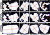 |
Fig. A.1. Comparison of three different eccentricity computation methods applied to four test segments. Top: Best-fit ellipse (image moments) approach. Middle: Extreme points using the centroid method. Bottom: Extreme points using the centroid method applied to convex hull image. The test segment 4 (rightmost column) corresponds to a special test showing a case where segmentation fails. |
To decide which method is better, further the visual decision explained in Fig. 4, we use other parameters, global shape descriptors as circularity (4πA/P2), where A is the area of the segment and P is its perimeter, and the solidity (A/Aconvex_hull) where Aconvex_hull is the area of the convex hull image of the segment. We also includes more sophisticated metrics, such as the Hausdorff distance (Taha & Hanbury 2015) and the chamfer distance transform (Chetverikov & Khenokh 1999), which are more sensitive to shape irregularities. With all those parameters, we calculated the pearson and spearman correlation coefficients with the multiple shape descriptors summarised in Table A.1
Summary of the correlations between each eccentricity e.
The correlation analysis shows in Table A.1 reveals that the custom eccentricity approach shows the best association with boundary irregularity measures, achieving spearman correlation of 0.458 with Hausdorff distance and 0.417 with chamfer distance. These values indicate that custom eccentricity effectively ranks shapes according to their boundary deviations, which represents more realistic shapes of the granular segments. Additionally, the negative correlation with circularity (-0.434) confirms that the metric also captures deviations from circular geometry. However, the notable Spearman correlation with area (0.352) suggests a dependency on segment scale. This must be due to segmentation failure detecting large artifact granules.
The convex hull-based eccentricity approach exhibits moderate performance across all correlation measures, providing a balanced characterisation. While its association with the shape descriptors, circularity, solidity, Hausdorff and chamfer distances, are less pronounced than those of the custom approach, this method demonstrates greater stability and reduced sensitivity to scale variations.
The ellipse-fitted eccentricity approach shows the weakest correlations with boundary irregularity measures, indicating limited capacity to detect structural deformations. Fitting an ellipse to the shape, smooths over boundary details and underestimates structural complexity. Consequently, while ellipse eccentricity may adequately describe simple elongation in smooth objects, it proves insufficient for applications for segments with irregular shape.
This comparative analysis establishes custom eccentricity as the optimal choice for combined elongation and irregularity detection, with convex eccentricity serving as a suitable alternative when shape-elongation measurement without scale dependency is more important.
All Tables
All Figures
|
Fig. 1. Left: Full-disk image context from the Helioseismic and Magnetic Imager (HMI) on board the Solar Dynamics Observatory (SDO). The red rectangle shows the region of interest observed by the 1-m SST. Right: Four-image grid displaying maps obtained from the SST data, including (a) blue-continuum intensity image, (b) strength of the magnetic field, (c) magnetic field inclination, and (d) magnetic field azimuth. |
| In the text | |
|
Fig. 2. Segmentation process of solar photospheric granules. (a) Original solar surface region. (b) Initial granule segmentation using local minima and the watershed technique. (c) Refined contour selection after parameter optimisation. (d) Final granule morphology after contour-based erosion. |
| In the text | |
|
Fig. 3. Granule area distributions. Top panel: Raw distribution of granule areas including outliers, with a fixed bin width of ∼0.15 arcsec2. Bottom panel: Histogram log(PDF) vs area, where the PDF is the normalised probability density of the area distribution. The dashed red line represents the fitting of the distribution to the derived parameters. |
| In the text | |
|
Fig. 4. 2D-log(KDE) plots showing the distribution of the areas and the three eccentricity metrics: (a) raw eccentricity (ellipse fitting), (b) convex eccentricity (computed on convex hulls), and (c) custom eccentricity (based on extreme points through the centre of mass of the segments). Each plot highlights the most probable eccentricity-area combinations and reveals trends. |
| In the text | |
|
Fig. 5. 2D-log(KDE) plots showing the dependence of: (a) granule area on granule eccentricity, (b) granule area on granule continuum intensity, (c) granule area on granule LOS velocity, and (d) granular continuum intensity on granule LOS velocity. Bottom: Dependence of granule (e) area, (f) continuum intensity, (g) LOS velocity, and (h) eccentricity on magnetic field strength. The colour-coding follows the same scheme, as in Fig. 4. |
| In the text | |
|
Fig. 6. 2D-KDE plots showing the dependence of area on eccentricity, segmented by horizontal magnetic field (Bhorizontal). Panel (a): 0–300 G,(∼58% of detected granules). Panels (b)-(f): Area-eccentricity relationship across different horizontal magnetic field ranges. The colour-coding follows that in Fig. 4. |
| In the text | |
|
Fig. 7. 2D-KDE plots illustrating the relationship between granule area and continuum intensity, and their dependence on the horizontal magnetic field. Panel (a) represents the 0–300 G range. Panels (b)-(f) show the evolution of the area-intensity relationship across other horizontal magnetic field ranges. The colour-coding follows that in Fig. 4. |
| In the text | |
|
Fig. 8. 2D-KDE plots showing the relationship between granule area and Δθ, as influenced by the horizontal magnetic field. Panel (a) covers 0–300 G. Panels (b)-(f) illustrate how the area–Δθ relationship evolves across different horizontal magnetic field ranges. The colour-coding follows that in Fig. 4. |
| In the text | |
|
Fig. A.1. Comparison of three different eccentricity computation methods applied to four test segments. Top: Best-fit ellipse (image moments) approach. Middle: Extreme points using the centroid method. Bottom: Extreme points using the centroid method applied to convex hull image. The test segment 4 (rightmost column) corresponds to a special test showing a case where segmentation fails. |
| In the text | |
Current usage metrics show cumulative count of Article Views (full-text article views including HTML views, PDF and ePub downloads, according to the available data) and Abstracts Views on Vision4Press platform.
Data correspond to usage on the plateform after 2015. The current usage metrics is available 48-96 hours after online publication and is updated daily on week days.
Initial download of the metrics may take a while.