| Issue |
A&A
Volume 708, April 2026
|
|
|---|---|---|
| Article Number | A53 | |
| Number of page(s) | 15 | |
| Section | Astrophysical processes | |
| DOI | https://doi.org/10.1051/0004-6361/202557681 | |
| Published online | 31 March 2026 | |
Evidence for cloud-to-cloud variations in the ratio of polarized thermal dust emission to starlight polarization
1
South African Astronomical Observatory, PO Box 9, Observatory, 7935, Cape Town, South Africa
2
Department of Astronomy, University of Cape Town, Private Bag, Rondebosch, 7701, Cape Town, South Africa
3
Department of Space, Earth and Environment, Chalmers University of Technology, 412 93, Göteborg, Sweden
4
Institute of Theoretical Astrophysics, University of Oslo, Blindern, Oslo, Norway
5
Université Libre de Bruxelles, Science Faculty CP230, B-1050, Brussels, Belgium
6
Université Paris-Saclay, Université Paris Cité, CEA, CNRS, AIM, F-91191, Gif-sur-Yvette, France
7
Department of Physics, University of Crete, Vasilika Vouton, 70013, Heraklion, Greece
8
Institute of Astrophysics, Foundation for Research and Technology – Hellas, 100 Nikolaou Plastira, Vassilika Vouton, 70013, Heraklion, Greece
9
University of Oxford, Denys Wilkinson Building, Department of Physics, Oxford, OX1 3RH, UK
10
Aix Marseille Univ., CNRS, CNES, LAM, Marseille, France
11
Department of Physics, University of Johannesburg, PO Box 524, Auckland Park, 2006, South Africa
12
Inter-University Centre for Astronomy and Astrophysics, Post bag 4, Ganeshkhind, Pune, 411007, India
13
Cahill Center for Astronomy and Astrophysics, California Institute of Technology, Pasadena, CA, 91125, USA
14
Jet Propulsion Laboratory, California Institute of Technology, 4800 Oak Grove Drive, Pasadena, CA, 91109-8099, USA
15
TAPIR, California Institute of Technology, MC 350-17, Pasadena, CA, 91125, USA
★ Corresponding author: This email address is being protected from spambots. You need JavaScript enabled to view it.
Received:
14
October
2025
Accepted:
15
February
2026
Abstract
The correlation between optical starlight polarization and polarized thermal dust emission can be used to infer intrinsic dust properties. This correlation is quantified by the ratio RP/p, which has been measured by the Planck Collaboration to be 5.42 ± 0.05 MJy sr−1 at 353 GHz when averaged over large areas of the sky. We investigated this correlation using newly published stellar polarimetric data densely sampling a continuous sky region of about four square degrees at intermediate Galactic latitude. We combined RoboPol optical polarization measurements for 1430 stars with submillimeter data from the Planck satellite at 353 GHz. We performed linear fits between the Planck (Qs, Us) and optical (qv, uv) Stokes parameters, taking into account the differences in resolution between the two datasets as well as the distribution of clouds along the line of sight. We find in this region of the sky that the RP/p value is 3.67 ± 0.05 MJy sr−1, indicating a significantly shallower slope than that found previously using different stellar samples. We also find significant differences in the fitted slopes when fitting the Qs–qv and Us–uv data separately. We explore two explanations using mock data: the miscalibration of the polarization angle and the variations in RP/p along the line of sight due to multiple clouds. We show that the former can produce differences in the correlations of Qs–qv and Us–uv, but large miscalibration angles would be needed to reproduce the magnitude of the observed differences. Our simulations favor the interpretation that RP/p differs between the two dominant clouds that overlap on the sky in this region. The difference in RP/p suggests that the two clouds may have distinct dust polarimetric properties. With knowledge from the tomographic decomposition of the stellar polarization, we find that one cloud appears to dominate the correlation of Us–uv, while both clouds contribute to the correlation of the Qs–qv data.
Key words: dust / extinction / ISM: magnetic fields / Galaxy: general / cosmic background radiation / cosmology: observations
Hubble Fellow.
© The Authors 2026
 Open Access article, published by EDP Sciences, under the terms of the Creative Commons Attribution License (https://creativecommons.org/licenses/by/4.0), which permits unrestricted use, distribution, and reproduction in any medium, provided the original work is properly cited.
This article is published in open access under the Subscribe to Open model. This email address is being protected from spambots. You need JavaScript enabled to view it. to support open access publication.
1. Introduction
Stellar polarization (due to dichroic extinction) and polarized thermal emission from dust grains are manifestations of the alignment of aspherical dust grains with the ambient Galactic magnetic field (Davis & Greenstein 1951; Lazarian 2007; Andersson et al. 2015). These polarized observables provide crucial insights into the structure of interstellar magnetic fields (Pattle et al. 2023) and the physical properties of dust grains (Draine 2003; Hensley & Draine 2021). Thus, understanding these phenomena is key to Galactic astrophysics and to the precise removal of foreground contamination in cosmological studies (Page et al. 2007; Planck Collaboration Int. XIX 2015; Planck Collaboration Int. XXI 2015).
The correlation between the plane-of-sky orientation of polarized dust emission and polarized starlight has been studied in a variety of regions (e.g., Soler et al. 2016). Less attention has been given to the correlation between the polarization amplitudes of these signals, even though a close link was anticipated (e.g., Martin 2007, and references therein). Planck Collaboration Int. XXI (2015) combined archival measurements of optical stellar polarization with polarized dust emission data at 353 GHz, and demonstrated that the Stokes parameters in absorption and emission are tightly correlated. Their correlation was quantified by the ratio of the polarized intensity of the emission (P) to the optical polarization fraction (p), RP/p = P/p. This ratio was found to have a value of approximately 5.4 ± 0.5 MJy sr−1 at 353 GHz (Planck Collaboration Int. XXI 2015). A later study (Planck Collaboration XII 2020) focusing on a sample of stars at high Galactic latitudes (Berdyugin & Teerikorpi 2001, 2002; Berdyugin et al. 2001, 2004, 2014) found a similar value of RP/p of 5.42 ± 0.05 MJy sr−1. The value of RP/p was found to be largely independent of column density (up to 10% variations), dust temperature, resolution, and Galactic latitude (Planck Collaboration Int. XXI 2015; Planck Collaboration XII 2020). This ratio has proven to be a powerful tracer of dust grain physics, providing constraints for parameters in dust models such as grain alignment efficiency, grain shape, and porosity (Guillet et al. 2018; Draine & Hensley 2021; Hensley & Draine 2023).
Beyond its role in dust astrophysics, this ratio could be used as a potential tool for modeling polarized foregrounds in cosmic microwave background (CMB) studies. However, for it to serve as a reliable predictor, its homogeneity across the sky must be established. Recent studies have reported spatial variations in the ratio in a small region of the diffuse interstellar medium (ISM) (Panopoulou et al. 2019a), and within a molecular cloud (Santos et al. 2017), suggesting that the assumption of a uniform correlation may not hold. These variations may be driven by changes in dust grain properties (e.g., Guillet et al. 2018; Draine & Hensley 2021) or by line-of-sight effects, where stars and dust emission trace different column densities in the three-dimensional ISM (Skalidis & Pelgrims 2019). Moreover, the wavelength dependence of stellar polarization (Serkowski et al. 1975) and the angular smoothing scale of the maps used for comparison can both influence the inferred ratio, adding further complexity to its interpretation.
For this work we investigated the possible variation of the ratio of polarized thermal dust emission at 353 GHz to optical starlight polarization using starlight polarization data within a continuous and extended region of approximately four square degrees. We combined starlight polarization measurements with Planck 353 GHz polarization maps (Nside = 2048, ∼5 arcmin) and pixel-averaged the data to a common Nside = 256 grid (∼14 arcmin) for the comparison. This region offers several advantages for our study as it is densely sampled by stellar polarization data and has a well-characterized three-dimensional magnetized ISM structure (Pelgrims et al. 2024). The latter was obtained from a tomographic decomposition of the stellar polarization (Pelgrims et al. 2023) as a demonstration of the capabilities of the PASIPHAE survey (Tassis et al. 2018).
The structure of the paper is as follows. Section 2 describes the datasets used in our analysis. Section 3 outlines the methodology. Section 4 presents the main results. Section 5 discusses the physical implications, and Sect. 6 concludes with a summary of our findings.
2. Data
2.1. Planck data products
We used full-sky submillimeter polarization data obtained by the Planck satellite, specifically from the fourth data release of the Planck collaboration (PR4) (Planck Collaboration III 2020). We used the single-frequency maps of Stokes Q, U at 353 GHz downloaded from the Planck Legacy Archive1. Galactic thermal dust emission dominates the polarized sky at 353 GHz (contributions from CMB polarization and polarized Cosmic Infrared Background (CIB) anisotropies are subdominant Planck Collaboration IV 2020).
The dataset consists of the Stokes parameters Is, Qs, and Us of the linear polarization of the dust emission and contains the per-pixel block-diagonal noise-covariance matrices between these observables. The data are provided at native resolution of the Planck mission, which adopts a HEALPix2 tessellation of the sphere with a resolution parameter of Nside = 2048 (Górski et al. 2005; Zonca et al. 2019). Since data are provided in units of KCMB, we multiplied them by a factor of 287.45 to convert them into MJy sr−1. This factor converts from thermodynamic temperature to specific intensity at 353 GHz, and was obtained from the Planck unit conversion and color correction tables, which account for the bandpass response of the High Frequency Instrument (HFI) and the non-linear relationship between temperature and intensity (Planck Collaboration IX 2014).
2.2. Optical starlight polarization catalog
We used the optical polarization catalog of Pelgrims et al. (2024). The catalog contains starlight polarization measurements and the corresponding uncertainties for 1698 stars over an area of approximately four square degrees (≈ 3° × 1.5°) centered on Galactic coordinates (l,b) ≈ (103.5°,22.25°) where l and b are the Galactic longitude and latitude, respectively. Measurements were made in the Johnson-Cousins R band using the RoboPol optical polarimeter (Ramaprakash et al. 2019) mounted at the 1.3 m telescope at the Skinakas Observatory3. The stellar polarization data are measured in the IAU convention (polarization angle measured from zero at the north and increasing towards the east). These measurements are provided in Equatorial coordinates, whereas the Planck data are in Galactic coordinates. For consistency, we transformed the stellar data to Galactic coordinates following the procedure described in Pelgrims et al. (2024).
We used Gaia EDR3 source identifier of stars given in the catalog to obtain distances from Bailer-Jones et al. (2021). There were 1675 stars with probabilistic distance estimates from Bailer-Jones et al. (2021). We used the photogeometric distance estimates from their work, which take into account both photometry and parallax information. From this set, we considered only the 1430 stars flagged as ‘ISM probe’ in the catalog compiled by Pelgrims et al. (2024), ensuring that the sample traces the dusty magnetized ISM and excludes intrinsically polarized stars (see Pelgrims et al. 2024 for details).
2.3. Star selection based on distance
As opposed to polarized dust emission, which probes the full column density up to infinity, starlight polarization only traces the dusty magnetized ISM up to the distances of the stars. To minimize any discrepancy between the amount of dust traced in absorption and in emission, we choose to select stars that likely trace most of the dust column, taking into account the knowledge of the 3D distribution of polarizing dust along the line of sight as reconstructed by Pelgrims et al. (2024). This approach differs from the one adopted in Planck Collaboration Int. XXI (2015), Planck Collaboration XII (2020) where the stellar polarization data were artificially corrected for the missing dust column by comparing the stellar extinction to the total extinction. This latter approach has limitations due to the available stellar-extinction maps and disregards possible depolarization effects due to variation of the plane-of-sky component of the magnetic field with distance.
Pelgrims et al. (2024) found that two clouds dominate the stellar polarization signal in this region of the sky. The first cloud is located at ∼58 pc (with considerable uncertainty as posterior distributions on its distance peak between 30 and 170 pc) and contributes, on average, a polarization fraction of 0.19% with an average polarization angle of 80°. The second, more distant, cloud is located at 374 pc (with estimates ranging between 354–448 pc). It contributes more significantly to the polarization, with a median polarization fraction of 1.45% and an average polarization angle of 40°. The two clouds cover the entire sky region considered in this work. To optimize the correlation between dust polarization in emission and absorption (starlight polarization), we selected stars with distances larger than 450 pc. This threshold corresponds to a distance beyond the 95th percentile of the cloud’s posterior distribution, which peaks at 374 pc, thus ensuring that the selected stars lie behind the cloud with high confidence.
More distant clouds were found towards distinct sightlines, at distances ranging from 1600 pc to 2400 pc in Pelgrims et al. (2024). These clouds can induce non-negligible polarization fractions (up to 0.58%) but only in few isolated regions of the map, each of size of approximately 10′. These very distant clouds affect only a small fraction of our stellar sample and should therefore only be considered as an additional source of noise in our analysis. To validate this assumption and check the robustness of our analysis with regard to these distant clouds, we also repeat our analysis with two other distance cuts, one demanding d > 2 kpc and the other d ∈ [450, 2000] pc.
To apply our distance cut, taking into account uncertainties on stellar distances, we used the lower and upper bounds of the photogeometric distance estimates from Bailer-Jones et al. (2021). Specifically, stars in the 450–2000 pc range are selected by requiring the lower bound (r_lo_photogeo) to be greater than 450 pc and the upper bound (r_hi_photogeo) to be less than 2000 pc, yielding a final sample of 929 stars. For stars confidently beyond certain thresholds, we rely solely on the lower bound: r_lo_photogeo > 450 pc results in 1200 stars, while r_lo_photogeo > 2000 pc results in 228 stars.
3. Methods
Planck Collaboration XII (2020) used starlight polarization data from a compilation of catalogs (Berdyugin et al. 2001, 2004, 2014; Berdyugin & Teerikorpi 2001, 2002) to compare against the Stokes parameters of the polarized dust emission. Unlike optical starlight data, which probes narrow lines of sight, Planck measurements average over larger beams (≳5 arcmin), leading to potential depolarization effects. To account for this, Planck Collaboration XII (2020) applied a correction factor to the Stokes parameters and associated uncertainties based on an analytical model of beam depolarization.
In our analysis, we did not apply this type of correction. Instead, we pixelized the optical and Planck data using the HEALPix scheme. The motivation for this pixelization is two-fold: (i) to improve the signal-to-noise ratio by averaging over several measurements per pixel and (ii) to ensure that each data point used in our comparison is as independent as possible. This is particularly important because the sampling of starlight polarization is often dense, with multiple stars falling within even a high-resolution Nside = 2048 pixel. After experimenting with different resolutions, we adopted Nside = 256 as a compromise between statistical independence and data quality. For example, approximately 80% of the pixels at Nside = 256 contain at least five stars, in contrast to Nside = 512, where 65% of the pixels contain fewer than five stars. Therefore, we expected to obtain more reliable statistical estimates at Nside = 256 and reduced sensitivity to beam mismatch effects between Planck and stellar polarization data (Planck Collaboration XII 2020).
3.1. Pixelization
Here, we describe the pixelization scheme used for both datasets. Although the method is generic, we adopt the convention that lowercase Stokes parameters (q, u) denote fractional optical starlight polarization, whereas uppercase Stokes parameters (Q, U) refer to Planck thermal dust emission at 353 GHz, expressed in MJy sr−1.
3.1.1. RoboPol data
The stellar polarization measurements are pixelized to create a HEALPix map at Nside = 256 (pixel size of ≈14′) as follows.
Suppose we have a total of N star measurements that can be distributed, according to their coordinates, across Npix pixels. The measured polarization (q, u) of each star i in the sample comes with uncertainties. In the Equatorial coordinate system there is no covariance between the measurements of q and u from the RoboPol instrument (Ramaprakash et al. 2019; Blinov et al. 2023). Therefore, the noise covariance matrix takes a diagonal form,
 (1)
(1)
which is no longer the case when the data is rotated to the Galactic reference frame (e.g., Pelgrims et al. 2024).
We assume that within a given pixel p, the ISM induces a polarization to the stars, described by a mean qp and up. We further assume that all variations in the observed stellar polarization arise solely from measurement uncertainties, which are normally distributed. We revisit and assess the validity of this assumption in Sect. 5.2. Our data model for each star measurement i can then be written as
 (2)
(2)
where N(μ, Σ) represents a random draw from a normal bivariate distribution with mean μ and covariance Σ. We also assume that the measurement uncertainties are independent, so that there is no covariance between measurements.
Given this model, an optimal estimator for the pixel weighted-mean polarization ⟨d⟩p ≔ (qp, up) is given by
 (3)
(3)
The covariance matrix corresponding to the weighted-mean polarization ⟨d⟩p is given by
 (4)
(4)
For diagonal covariance matrices Cqu, i, this resolves trivially into a set of scalar equations.
In the remainder of this work, we denote the pixel-averaged fractional Stokes parameters derived from the RoboPol data as qv and uv, where the subscript ‘v’ indicates starlight polarization in the visible. These correspond to the quantities qp and up defined above. The associated uncertainties on these parameters are denoted as σqv2 and σuv2, obtained from the diagonal elements of the pixel-averaged covariance matrix Cqu, p. Since the stellar measurements are rotated into the Galactic coordinate system, we also retain the off-diagonal term, denoted as σquv, which contributes to the joint error analysis (see Sect. 3.3).
3.1.2. Planck data
The Planck data are processed in a manner similar to the RoboPol data. The maps are provided at a native resolution of Nside = 2048, where each pixel is treated as an independent measurement of the Stokes parameters Q and U.
Since Planck follows the HEALPix convention, we convert to the IAU system by multiplying the values of U by −1 prior to any further processing.
For the comparison with the RoboPol data, we construct a lower-resolution map of Nside = 256, where values of the original map are averaged in larger pixels. At this resolution, each large pixel at Nside = 256 encompasses 64 smaller pixels from the original Nside = 2048 map. These smaller pixels are treated as independent measurements (analogous to individual stars), and their values are grouped using Eqs. (3) and (4).
In the remainder of this work, we denote the pixel-averaged Planck Stokes parameters as Qs and Us (s is used to denote submillimeter polarization). The associated uncertainties on these parameters are denoted as σQs2 = CQQ and σUs2 = CUU, which are the diagonal elements of the pixel-averaged covariance matrix. The off-diagonal term of this matrix is denoted as CQU.
3.2. Comparison of dust polarization in emission and absorption
To compare the Planck data with starlight polarization, we aim to measure the polarization ratio RP/p, which in principle could be estimated by correlating the polarized intensity in emission with the polarization fraction in extinction. However, both the polarized intensity and the polarization fraction are non-linear combinations of the Stokes parameters and are positively biased in the presence of noise. In contrast, the Stokes parameters have Gaussian noise properties. Following Planck Collaboration Int. XXI (2015), we therefore quantify the emission–absorption relationship by correlating the emission Stokes parameters (Qs, Us) with their optical fractional counterparts (qv, uv), which is directly related to RP/p in the idealized case of orthogonal polarization, as shown below.
The optical Stokes parameters are defined as qv = pcos2ψv and uv = psin2ψv, where ψv is the polarization angle in extinction, while ψs is used to denote the polarization angle in emission. In the ideal case where noise is negligible and the polarization pseudo-vectors in extinction and emission are orthogonal (ψs = ψv + π/2), one has
 (5)
(5)
 (6)
(6)
(up to the sign convention adopted for U). Thus, the slopes of the correlations Qs versus qv and Us versus uv both yield unbiased estimates of the same physical ratio RP/p. In practice, this correlation analysis is performed on the pixelized maps constructed as explained in Section 3.1.
We identify the HEALPix pixels that have at least one stellar polarization measurement. We include the Planck data at those pixels in our analysis. Following the pixelization procedure outlined above, the resulting pixelized maps for RoboPol and Planck are shown in Fig. 1. These maps depict the Gnomonic projections of the pixelized Stokes parameters for the sky patch observed by RoboPol and Planck at Nside = 256, using stars with distance to the Sun greater than 450 pc. The maps are centered at coordinates (l, b) = (103.5° , 22.5° ). White pixels indicate regions outside RoboPol’s observed sky area. Notably, these maps highlight a clear anti-correlation between the Planck Stokes parameters and the optical fractional Stokes parameters, with Pearson correlation coefficients of the pairs of data (Qs, qv) and (Us, uv) being rQ = −0.83 and rU = −0.84, respectively. We explore these correlations in the following sections.
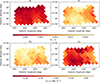 |
Fig. 1. Gnomonic projections of the pixelized Stokes parameter data at optical (top) and submillimeter (bottom) at Nside = 256 and distance cut > 450 pc. Top left: qv; Top right: uv; Bottom left: Qs; Bottom right: Us. The Stokes parameters follow the IAU convention. Pixels with no optical data (outside of the observed sky region) are white. |
3.3. Fitting procedure
The pixelized polarization data from Planck and RoboPol are shown in Fig. 2 in pairs of (Qs, qv) and (Us, uv) and display a linear relationship, as expected. To study this correlation and determine the ratio of polarized emission to optical polarization RP/p, we perform a fit of the form y = ax + b. Here, a represents the ratio of polarized emission to optical polarization (RP/p), while b accounts for any offset between the two datasets.
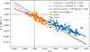 |
Fig. 2. Correlation between the Stokes parameters from Planck (Qs, Us) and the fractional Stokes parameters from RoboPol (qv, uv). The blue points represent the correlation between Us and uv, while the orange points show the correlation between Qs and qv. The blue dashed line indicates the best-fit line of the joint correlation determined by minimizing χ2, while the solid blue and solid orange lines correspond to the Us − uv and Qs − qv fits, respectively. The black dashed line corresponds to the value from Planck Collaboration XII (2020). |
We perform independent linear fits to the (Qs, qv) and (Us, uv) datasets using the Bayesian hierarchical regression method LinMix (Kelly 2007). The prior on the independent variable is represented as a mixture of two Gaussians, K = 2, while the slope a and intercept b are assigned broad, non-informative priors. Posterior samples of the slope a and intercept b are obtained using a Markov Chain Monte Carlo (MCMC) maximum-likelihood analysis. We report the posterior median as the best-fit value, with the posterior standard deviation representing the associated uncertainty.
To estimate a value of RP/p, we also perform a joint fit to both Stokes parameters using a custom MCMC sampler implemented via emcee (Foreman-Mackey et al. 2013). This approach follows the methodology outlined in Planck Collaboration Int. XXI (2015). It models the combined system of (qv, uv) and (Qs, Us) using a shared slope a, a common offset b, and incorporates the full covariance matrix of Planck uncertainties (CQQ, CUU, CQU), along with the variances from the stellar measurements. The likelihood is constructed from a chi-square function of the residuals, defined as
 (7)
(7)
where V(a,b) and M(a,b) are defined as
We report the median and standard deviation of the posterior samples for both the joint fit slope and intercept as our final results.
4. Results
4.1. Correlation analysis
Figure 2 presents the correlation between the Planck Stokes parameters (Qs, Us) and the RoboPol fractional Stokes parameters (qv, uv), for stars located beyond 450 pc, as computed in Sect. 3. We show scatter plots of the paired values, along with best-fit linear relations. Both individual fits to Qs versus qv and Us versus uv, as well as a combined joint fit to all (Qs, Us) versus (qv, uv) pairs, are presented. For brevity, we denote the fitted slopes as RQq, RUu, and RP/p, corresponding to the Qs versus qv, Us versus uv, and joint (Qs, Us) versus (qv, uv) fits, respectively. Table 1 summarizes the results of these fits.
Summary of results from the fitting.
The plots reveal a strong anti-correlation between the datasets. A joint fit yields a slope of −3.67 ± 0.05 MJy sr−1, significantly different from the −5.42 MJy sr−1 value found in Planck Collaboration XII (2020). When fitted separately, the slopes are approximately −5.13 ± 0.4 MJy sr−1 for Qs versus qv, and −3.64 ± 0.2 MJy sr−1 for Us versus uv. Notably, RQq is consistent with the Planck result, while RUu remains significantly different.
The uncertainty on the slope RQq is higher compared to the joint and RUu fits. This can be attributed to two factors: the median signal-to-noise ratio in qv is 8 times lower than that of uv and the fact that qv data span a narrower range of values than uv: the interquartile range of qv is 0.0028, while that of uv is 0.0068. The combined joint fit benefits from the broader range, resulting in a notably smaller uncertainty of 0.05 MJy sr−1r, compared to approximately 0.4 MJy sr−1 for RQq. Despite the larger uncertainties, the detected slopes for both Qs−qv and Us−uv relations are statistically highly significant, and the differences between them are not attributable to fitting uncertainties.
In all cases, a small but non-zero intercept is required for an optimal fit. Fixing b = 0 results in significantly worse fits, as reflected in much higher minimum χ2 values. For the Qs versus qv relation, the minimum χ2 decreases by a factor of 1.61 when allowing b ≠ 0. In the joint fit of (Qs, qv) and (Us, uv), the improvement is much more substantial, with the χ2 dropping by a factor of about 35.4. In contrast, for the Us versus uv fit, the change is modest (a factor of 1.07), suggesting that the intercept plays a less critical role in that case.
As discussed in Sect. 3, it is important to check the robustness of our results against the distance-selection criterion. Therefore, we repeat our analysis with different distance selections, the results of which are summarized in Fig. 3 where we show the variation of the fitted slope values as a function of different distance cuts. The slopes RUu and RP/p are mutually consistent within 1σ across the distance selections. In contrast, RQq varies with the distance cut: the > 2000 pc selection yields a slope that is inconsistent with both the > 450 pc and 450 − 2000 pc cuts and with the Planck value, whereas the latter two cuts remain mutually consistent (within 1σ). These results confirm that our primary conclusion is robust to distance selection: the Qs−qv and Us−uv correlations have significantly different slopes, and the joint slope differs from the Planck value.
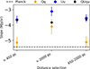 |
Fig. 3. Comparison of best-fit slope values for different star sample selections. All cases are analyzed at the same Nside of 256. The slope found in Planck Collaboration XII (2020) is shown as the black dashed line. |
In addition, we repeat the analysis at NSide = 512, where we observe a slight flattening of the RQq slope compared to the results presented above, while RUu and RP/p remain largely unchanged. We also experimented with different approaches for estimating the mean Stokes parameters per pixel, including the method of Gatz & Smith (1995) and the inverse-variance weighting described in Sect. 3.1.1. The results of these validation tests were found to be consistent within 1σ for the distance cuts of > 450 pc and 450–2000 pc. However, for the > 2000 pc cut, we obtain higher values, the details of which are discussed in Appendix B.
4.2. Angle differences with Planck
In the previous section, we noted a difference between the joint slope RP/p in our dataset and that reported by Planck Collaboration Int. XXI (2015) over a larger region of the sky. One possible explanation for this discrepancy could be that optical polarization from stars in our sample, may not be probing the entire column of dust traced by the submillimeter polarization from Planck along the line of sight (LOS) (Skalidis & Pelgrims 2019).
If the polarized emission arises from the same region that causes the polarization of starlight in absorption, the polarization angles from both types of data should differ by 90°. To test this, we compute the angle differences between starlight and Planck polarization for our different distance-cut criteria that select the stars that contribute toward the pixelized RoboPol data. We estimate the angle difference ΔΨs/v defined from the Stokes parameters and introduced in Planck Collaboration Int. XXI (2015) as4
![Mathematical equation: $$ \begin{aligned} \Delta \Psi _{s/v} = \frac{1}{2} \text{ atan2} [(U_s q_v - Q_s u_v), -(Q_s q_v + U_s u_v)]. \end{aligned} $$](/articles/aa/full_html/2026/04/aa57681-25/aa57681-25-eq28.gif) (8)
(8)
This angle difference is defined in the range −90° to 90° and takes a value of 0 when the polarized emission and absorption are perpendicular.
We compare the stellar polarization angles, using all the stars located beyond 450 pc, with those measured by Planck (after conversion to the IAU convention). The distribution of the angle differences (ΔΨs/v) is shown in Fig. 4 (right). We find a median offset of 4.0°. A similar offset between stellar and Planck polarization angles was found by Planck Collaboration XII (2020). Their distribution of ΔΨs/v peaked at −3.1°, a sign flip relative to our result due to the convention used, indicating a small systematic shift between the polarization angles measured in emission versus extinction. Planck Collaboration XII (2020) commented on the fact that such an offset may arise from differences in angular resolution and probed distances (beam effects) or potential residual systematics in the determination of the zero-point polarization angle of the optical data, or variations of magnetic field/dust properties along the line of sight.
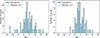 |
Fig. 4. Distributions of ΔΨs/v (in degrees) for stars with distance d ≥ 2000 pc (left) and d ≥ 450 pc (right). The red vertical lines indicate the distribution’s median; the values are reported in the legend. |
To investigate whether this offset is due to some stars in our sample not tracing the full column, we examine the angle differences for stars located at greater distances (beyond 2 kpc) compared to the Planck data. As shown in Fig. 4 (left), the offset decreases to a median value of 3.2°. Accounting for a sign flip, the offset that we observed is small and consistent in magnitude with that reported by Planck Collaboration XII (2020). A Kolmogorov–Smirnov (K-S) test between the distributions of ΔΨs/v for the 450–2000 pc versus the > 2000 pc samples shows that the distributions are consistent with each other (K-S statistic of 0.13 and a p-value of 0.44). This suggests that the choice of distance cut does not strongly affect the overall ΔΨs/v distribution and that differences in distance alone do not explain the observed angle offset. Furthermore, since stars beyond 2 kpc may lie behind the furthest clouds in the region (Pelgrims et al. 2024), it is unlikely that incomplete column tracing is responsible for the slope discrepancy seen between our fits and those of previous works.
Therefore, the small median angle offset is more likely due to beam mismatch, bandpass mismatch or residual miscalibration errors, rather than the distance selection of the stars. However, we expect beam-related effects to be subdominant at the coarse angular resolution adopted in this work (Nside = 256, ∼14 arcmin). We verified this by performing Gaussian-smoothing tests, which did not affect our main results. We also considered the potential impact of bandpass mismatch. Throughout this work, we used the Planck PR4 polarization maps, in which bandpass mismatch is explicitly modeled and corrected during mapmaking. As an additional check, we repeated the analysis using PR3 maps, for which such corrections are less complete, and found consistent results. In particular, the observed difference between RQ/q and RU/u remains unchanged. This leaves residual miscalibration as a more plausible contributor to the observed offset. In addition, variations in dust properties (e.g., composition or alignment efficiency) across clouds may also contribute to its origin. In the following section, we explore these possibilities in more detail.
4.3. Exploring the origin of the difference between RQq and RUu
In Sect. 4.1, we found a significant difference between the slopes for the Qs−qv and Us−uv and non-zero intercepts, as well as a significantly different RP/p compared to that found by Planck Collaboration Int. XXI (2015), Planck Collaboration XII (2020). We have verified that our methodology reproduces results compatible with the Planck analysis when applied to that same dataset using two different versions of the Planck data (see Appendix A). This confirms that the differences in our findings are not due to methodological choices or changes in the systematic uncertainties of the Planck data. The ‘atypical’ RP/p value also cannot arise from the wavelength-dependent variations of the starlight polarization (Serkowski et al. 1975), as the differences between the bandpass of the RoboPol data (R-band) compared to those used in the stellar surveys employed in the analysis of Planck Collaboration Int. XXI (2015), Planck Collaboration XII (2020) are small.
We propose and explore two possible reasons to explain the differences in slopes–both between our results and those from Planck, and between our Qs−qv and Us−uv relations, namely a miscalibration of the zero angle and line-of-sight variations of the dust properties.
4.3.1. Effect of zero-point angle miscalibration
The method for calibrating the zero-point of the polarization angle differs significantly between the Planck and optical polarization data. The latter are calibrated against ‘known’ standard stars, and may have residual systematic uncertainties at the level of 1° (but can be higher depending on the calibrator stars used, Blinov et al. 2023).
We investigate the potential effect of a miscalibration of the zero-point polarization angle on the correlation between starlight polarization (qv, uv) and dust emission (Qs, Us) using a toy model. We introduce an offset angle (β) in the polarization plane, and produce mock observations of stellar polarization and polarized dust emission. We then demonstrate that the measured Stokes parameters undergo a systematic rotation, altering the observed slopes and intercepts in the regression analysis.
We generated 500 random realizations of position angles and polarization degrees, drawn from normal distributions:
 (9)
(9)
For these simulations, we adopted two values of the mean polarization angle: ΨB⊥ = 30° or 60°, with a standard deviation of  . The polarization degree p was drawn from a normal distribution, with two cases considered: one with a mean of 2.5% and another with a mean of 1.5%, both with a standard deviation of σp = 0.2%. Using these values, we computed the stellar reduced Stokes parameters in the IAU convention as
![Mathematical equation: $$ \begin{aligned} \begin{pmatrix} q_v \\ u_v \end{pmatrix} = p_v \begin{pmatrix} \cos {[2\Psi _v]} \\ \sin {[2\Psi _v]} \end{pmatrix}. \end{aligned} $$](/articles/aa/full_html/2026/04/aa57681-25/aa57681-25-eq31.gif) (10)
(10)
Next, we introduce a single RP/p value (5.42 MJy sr−1) and compute the corresponding Stokes parameters for dust emission:
 (11)
(11)
Then a miscalibration in the zero-point of the polarization angle is introduced. To model this calibration error, we assume that the polarization angle is offset by an angle β. This results in a rotation of the measured Stokes parameters relative to their true values:
 (12)
(12)
We analyze the simulated data in the same way as the actual data, and Fig. 5 illustrates the results, showing both the fitted slopes and the resulting intercepts for various misalignment scenarios. For different values of the magnetic field position angle (ΨB⊥), degree of polarization (p), and miscalibration offset (β), we found that small calibration errors can impact the inferred relationships between (Qs, qv) and (Us, uv). The effect becomes more pronounced for larger miscalibration angles and higher degrees of polarization, leading to variations in the slopes and intercepts of the fitted correlations. For simplicity, the miscalibration angle that we introduced in our toy model affects only the simulated dust emission data. A similar approach could be applied to the stellar polarization or both. Furthermore, no noise was added to the data in the above exercise. Therefore, when computing the difference in the position angle of the magnetic field inferred from dust emission and from the stars, we always obtain a consistent and unique value equal to the imposed offset. Although the true relation between our simulated submillimeter and optical Stokes parameters is strictly linear and passes through the origin, our fits yield a non-zero intercept. These simulations demonstrate that differences in the slopes of the Qs–qv and Us–uv correlations can arise from a miscalibration in the zero-point of the polarization angle, particularly when the polarization degree p is relatively high (e.g., 2.5%) and the miscalibration angle β is large (e.g., 7°; see the fourth column of the second row in Fig. 5). However, in our dataset, the typical polarization degrees are closer to 1.5% and the miscalbration angle β can be up to ∼ 3° (see Fig. 4). This would correspond to the first and third column of the first row in Fig. 5. Large systematic miscalibration angles are unlikely given current calibration standards (Blinov et al. 2023). Therefore, while our model demonstrates that miscalibration can induce an asymmetry between the two correlations, the size of the miscalibration required to reproduce the observed differences in our data appears unrealistically large. This suggests that zero-point angle miscalibration alone is unlikely to fully account for the observed slope differences, and that additional physical or observational factors must be at play.
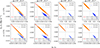 |
Fig. 5. Correlation plots and linear fits between (Qs, qv) and (Us, uv) for two values of the polarization degree, p = 1.5% (top row) and p = 2.5% (bottom row). Each column corresponds to a combination of magnetic field orientation ΨB⊥ = {30°, 60°} and miscalibration offset β = {3°, 7°}, increasing from left to right. The best-fit values for the slopes (absolute value) and for the intercept obtained for the correlations are given in the legend; the resulting model is shown on the scatter plot, in blue for (Qs, qv) and in orange for (Us, uv). They are expressed in MJy sr−1. To generate the data, we used Rp/p = 5.42 MJy sr−1, σΨB⊥ = 5°, and σp = 0.2% to produce the dynamical range. |
4.3.2. Evidence for cloud to cloud variations in RP/p
Here we present arguments to explain the origin of the difference in slopes between the Qs–qv and Us–uv data in terms of a variable RP/p in clouds along the line of sight.
Analyses of stellar polarimetry, distances and H I emission spectra showed the presence of multiple clouds at different distances in the region under investigation (Panopoulou et al. 2019b; Pelgrims et al. 2023, 2024). In particular, Pelgrims et al. (2024) found that the majority of the area is occupied by two clouds at different distances, that overlap on the plane of the sky, producing distinct signatures in the Stokes parameters of the stellar measurements. From their result, we can infer that the observed polarized dust emission (for a given pixel) will be the result of the contribution of the individual cloud contributions:
 (13)
(13)
 (14)
(14)
where Qs, Us are the observed Stokes parameters from Planck and Q(1), U(1), Q(2), U(2) are their individual contributions from the two clouds having different distances. In what follows, we label the nearest cloud with the index 1, and the farther cloud with index 2.
We also expect that the Stokes parameters of the emission of each cloud will be related to those of the absorption arising from each cloud via a ratio RP/p:
 (15)
(15)
 (16)
(16)
Here,  and
and  are the stellar Stokes parameters for cloud 1 (with Q(1), U(1) the corresponding emission), and
  and
and  are for cloud 2 (with Q(2), U(2) the corresponding emission).
  is the ratio for the first cloud and
  the ratio for the second cloud along the line of sight (LOS). We note that dust properties may vary from cloud to cloud; therefore we allow different slopes when modeling different clouds. However, within a given cloud the dust properties are expected to be uniform, and we thus adopt the same slope for both Stokes parameters.
Combining the above sets of equations, we can write the observed Stokes parameters of the emission as:
 (17)
(17)
Up to this point we have made no assumptions about the relationship between the ratios  and
and  of the two clouds.
Next, we assume that  and will show that this leads to a contradiction with the data. Under this assumption, we can re-write Eq. (17) as:
 (18)
(18)
Thus, our assumption of the two clouds having the same ratio R implies that we should measure the same slope for the Qs–qv and Us–uv data. This is incompatible with the results obtained in Sect. 4.1, what leads us to conclude that the polarization ratios in cloud 1 and 2 are different ( ).
).
If a tomographic decomposition of the stellar polarization Stokes parameters is available, one can use it to fit for the unknown ratios  via Eq. (17). We investigate how such information can be used to explain the observed discrepancy between the Qs−qv and Us−uv slopes found in Sect. 4.1.
The tomographic decomposition of Pelgrims et al. (2024) showed that for all pixels in the map
 (19)
(19)
The second cloud appears to dominate the signal in uv, due to its particular magnetic field geometry (forming an angle of ∼40°) and its higher p compared to the first cloud (1.4% compared to 0.2%). This allows us to simplify the system in Eq. (17). If we assume that  and
and  are of the same order of magnitude (so that
  ) we obtain:
 (20)
(20)
 (21)
(21)
because in this region uv ≈ uv(2), the second of these equations shows that the observed Us−uv slope in our dataset is representative of the second cloud.
We verify this conclusion by creating mock data for our two-cloud hypothesis, where the clouds may possess different intrinsic properties – such as porosities, temperature or shape (Draine & Hensley 2021) – that result in distinct RP/p values and, consequently, affect the observed correlations. The observed Stokes parameters are expressed as the sum of contributions from two separate clouds:
 (22)
(22)
 (23)
(23)
The relative contribution from each cloud depends on the degree of polarization (pv(i)) and the plane-of-sky magnetic field orientations in both absorption and emission. We chose the values for the degree of polarization (p[1],p[2]) and polarization angles (![Mathematical equation: $ \Psi_{B\perp}^{[1]} $](/articles/aa/full_html/2026/04/aa57681-25/aa57681-25-eq59.gif) ,
, ![Mathematical equation: $ \Psi_{B\perp}^{[2]} $](/articles/aa/full_html/2026/04/aa57681-25/aa57681-25-eq60.gif) ) based on the tomographic decomposition presented by Pelgrims et al. (2024). We adopt an RP/p value for the second cloud that is equal to the slope found in the Us − uv correlation. For the first cloud, we adopt RP/p = 5.4 MJy sr−1, similar to the value found by Planck.
) based on the tomographic decomposition presented by Pelgrims et al. (2024). We adopt an RP/p value for the second cloud that is equal to the slope found in the Us − uv correlation. For the first cloud, we adopt RP/p = 5.4 MJy sr−1, similar to the value found by Planck.
Fig. 6 illustrates an example of the resulting correlation plot for a case with p[1] = 0.2%, p[2] = 1.4%, ![Mathematical equation: $ \Psi_{B\perp}^{[1]} = 80\circ $](/articles/aa/full_html/2026/04/aa57681-25/aa57681-25-eq61.gif) ,
, ![Mathematical equation: $ \Psi_{B\perp}^{[2]} = 40\circ $](/articles/aa/full_html/2026/04/aa57681-25/aa57681-25-eq62.gif) , and
, and ![Mathematical equation: $ R_{P/p}^{[1]} = 5.4 $](/articles/aa/full_html/2026/04/aa57681-25/aa57681-25-eq63.gif) ,
, ![Mathematical equation: $ R_{P/p}^{[2]} = 3.7 $](/articles/aa/full_html/2026/04/aa57681-25/aa57681-25-eq64.gif) . We generate 500 synthetic measurements (without added noise) using
. We generate 500 synthetic measurements (without added noise) using ![Mathematical equation: $ \sigma_{\Psi_{B\perp}}^{[i]} = 2\circ $](/articles/aa/full_html/2026/04/aa57681-25/aa57681-25-eq65.gif) , σp[1] = 0.2%, and σp[2] = 0.2%. This example produces results qualitatively similar to the data of Fig. 2. The measured slope for (Us, uv) is close to the value assumed for cloud 2.
, σp[1] = 0.2%, and σp[2] = 0.2%. This example produces results qualitatively similar to the data of Fig. 2. The measured slope for (Us, uv) is close to the value assumed for cloud 2.
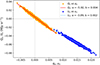 |
Fig. 6. Correlation plot for the simulated example of two intervening clouds with different polarization properties and different RP/p ratios, as described in the text. |
A non-zero intercept also arises in this case, as illustrated in Figure 6. This becomes evident when we express Eq. (17) in terms of the observed Stokes parameters. For example:
 (24)
(24)
 (25)
(25)
 (26)
(26)
Here, qobs is the total observed stellar Stokes parameter. When expressing Qs as a function of qobs, the mismatch between the relative contributions of the two clouds introduces an intercept term proportional to  , even though the underlying physical relation among the components contains no intercept.
This analysis confirms that variations in RP/p across multiple clouds can produce different RQq versus RUu. The variations in slopes and intercepts combined with a tomographic decomposition of the optical polarization Stokes parameters could be used to infer properties of the dust, grain alignment and magnetic fields as they vary along the line of sight.
5. Discussion
In Sect. 4, we investigated the correlation between optical and submillimeter polarization Stokes parameters in a localized region of the diffuse ISM. Interestingly, not only did we find a value that differs from that reported previously in different sky regions (Planck Collaboration Int. XXI 2015; Planck Collaboration XII 2020), but we also observed different slopes for the RQq and RUu correlations. We explored various potential explanations for this discrepancy, ruling out the possibility that optical polarization does not trace the full column of dust probed by submillimeter polarization along the LOS (Sect. 4.2). We suggest a combination of low-level zero-point angle miscalibration (Sect. 4.3.1) and variations in dust properties along the LOS (Sect. 4.3.2) as a likely origin of the trend reported in Sect. 4.1.
In Planck Collaboration Int. XXI (2015) only a slight difference in the slopes of (Qs, qv) and (Us, uv) was found, along with the possibility of a small intercept. They compared starlight polarization and dust emission along translucent sightlines at low Galactic latitude, finding slopes of RP/p = ( − 5.17 ± 0.09) MJy sr−1 and ( − 5.07 ± 0.13) MJy sr−1 for the two correlations. The corresponding y-intercepts were found to be (0.0077 ± 0.0013) MJy sr−1 and ( − 0.0016 ± 0.0013) MJy sr−1. These differences are small compared to the associated uncertainties. More significant differences between RQq and RUu were found by Versteeg (2025) when comparing NIR stellar polarimetry from Clemens et al. (2020) with polarized dust emission from Planck.
5.1. On the atypical RP/p
In Sect. 4.3.2, we demonstrated using simulated data how clouds with different values of RP/p can effectively reproduce our observational results. Based on these findings, the question arises of why the RP/p value of the second cloud is so much lower than the typical value of 5.4 MJy sr−1. Indications of a lower RP/p of 4.2 ± 0.1 MJy sr−1 in the diffuse ISM were also found in a different region of the sky (Panopoulou et al. 2019a).
First, we expect that the observation of a lower value of RP/p (in our study ∼3.7 MJy sr−1) compared to the typical value, is likely due to an increased optical polarization relative to FIR polarized intensity. The polarized intensity spectrum depends mostly on the dust temperature Td. At 353 GHz the polarized intensity is proportional to the grain temperature: P ∝ Td. The grain temperature relates to the strength of the radiation field, J, as J ∝ Td5.5 (Draine 2011). In order for RP/p to decrease by a factor of 1.5, the radiation field would have to decrease by a factor of almost 10, which seems unrealistic for the diffuse ISM.
Another factor affecting both the optical and FIR polarization is the minimum size of aligned grains, which determines the mean alignment efficiency (e.g., Hensley & Draine 2023). In the FIR, the amplitude of the polarized intensity spectrum increases proportionally to the mean alignment efficiency. The shape of the optical polarization spectrum is also sensitive to the mean alignment efficiency, in a more complex way (e.g., Reissl et al. 2020). We have investigated the effect of changing the minimum size of aligned grains on RP/p in the context of the Astrodust model (Hensley & Draine 2023). We find that varying the minimum size of aligned grains in the range of 0.01–0.08 μm has a minimal effect, far too small to explain the observed change in RP/p of a factor of 1.5.
The shape of the optical polarization curve is sensitive to the shapes and porosities of grains while the polarized intensity spectrum is largely insensitive to these variations (e.g., Voshchinnikov 2012; Guillet et al. 2018; Draine & Hensley 2021). Given this, one might wonder whether there is independent evidence that dust properties (such as their size distribution) are ‘atypical’ in the region under investigation. The cloud with anomalous RP/p is part of the Cepheus Flare where the ratio of total to selective extinction, RV, appears to be lower than the mean diffuse ISM value of 3.1: based on the map of Zhang & Green (2025) we find a mean RV in the region at 400–500 pc of 2.6. Since RV is known to reflect the grain size distribution (Mathis et al. 1977; Mathis & Wallenhorst 1981; Kim et al. 1994), the lower RV could indicate an increased population of smaller grains.
However, in the translucent ISM with 1 ≤ AV ≤ 3 mag, variations in RV may instead be driven by changes in the abundance of Polycyclic Aromatic Hydrocarbons (PAHs; Zhang et al. 2025), which affect extinction but not polarization. The cloud under investigation is even more diffuse, with extinction ranging from 0.4–0.5 mag between 400 and 1000 pc based on the Zhang & Green (2025) map. Changes in the PAH population would not reflect in RP/p, which mainly traces the aligned, larger grains (Hensley & Draine 2023).
Thus, the low RP/p value in our study suggests the presence of a population of aligned dust grains in this region that are atypical compared to those in the general ISM. At the same time, it is unclear whether the extinction curve supports such a different population of grains. To test our hypothesis, multiwavelength observations of the optical polarization of stars tracing the cloud would be invaluable. By measuring the wavelength-dependence of the optical polarization curve, one would be able to estimate the wavelength where maximum polarization occurs, λmax. Correlations between λmax and RV (Whittet & van Breda 1978) have been linked to variations in the sizes and properties of aligned grains. If the linear correlation between RV and λmax found by Serkowski et al. (1975) and Whittet & van Breda (1978) holds5 and if it can be extrapolated to lower AV (these studies typically used stars at AV ∼ 1 mag or higher), then an RV of 2.6 would imply a λmax of 0.46 μm in this cloud, compared to the typical 0.55 μm value. To properly estimate the λmax of the dominant cloud along the LOS, one would also have to correct for the effect of the foreground cloud on the wavelength-dependence of the polarization (Mandarakas et al. 2025; Skalidis 2024). To explore a potential connection between RV and RP/p multiband optical polarization measurements are required across many more regions.
5.2. Assessing the impact of small-scale variations
In the model for estimating the stellar polarization within a given pixel, we make several assumptions. In particular, we assume that the measurements within each pixel contain no additional sources of variability beyond instrumental noise, and that this noise is correctly estimated by the RoboPol pipeline.
To test this assumption, we perform a goodness-of-fit test before rotating the measurements (so that the q–u covariance matrices remain diagonal). Specifically, for each individual pixel, we compute the reduced chi-squared statistic:
 (27)
(27)
Here di is the individual measurement vector of the stars, ⟨d⟩ is the pixel-averaged value, and Cqu, i is the noise covariance matrix for each stellar measurement.
If the noise is properly characterized and dominates over any intrinsic scatter, we expect χd.o.f.2 ≈ 1. However, we find that the median value of χd.o.f.2 over the full area to be approximately 2.46. The corresponding value for the Planck data is very close to unity. This suggests that the stellar data, probing pencil-beams, reveal significant intrinsic scatter within pixels, whereas the Planck data remains noise-dominated.
To account for this apparent underestimation of the uncertainties in the stellar data, we explore inflating the errors by adding an intrinsic scatter term to the covariance matrix,
 (28)
(28)
where vc is chosen such that Eq. (27) yields χd.o.f.2 ≈ 1.
While this approach helps in principle, it oversimplifies the problem. Intrinsic scatter may not affect the diagonal terms ( ,
,  ) equally and can also introduce a non-zero off-diagonal term (
 ), though typically of smaller amplitude (see Appendix B of Pelgrims et al. 2023 for a detailed toy model-based discussion on this matter). Estimating the full intrinsic covariance matrix for each pixel would require numerically solving for all three components (
 ,
,  , and
, and  ) by maximizing the log-likelihood for each pixel. If one assumes Gaussian statistics for the intrinsic scatter in the q and u measurements, the problem can be somewhat simplified (Skalidis et al. 2018), however the reliability of this assumption needs further testing. Therefore, due to the complexity of this method and the lack of a robust way to constrain all three elements of the covariance matrix reliably for each pixel, we opted not to implement the full error inflation scheme.
We did, however, test the simplified inflation approach described above and found that the resulting slopes were consistent with those obtained using the un-inflated uncertainties in Sect. 4.1, with deviations well within 1σ. This confirms that our main results are robust against modest underestimation of uncertainties. Given the small impact on the final results, we adopt the un-inflated inverse-variance approach as our default method for simplicity. Future improvements to this analysis could incorporate full intrinsic covariance estimation and more realistic modeling of small-scale correlations.
6. Summary
In this paper, we estimated the ratio of polarized thermal dust emission to optical starlight polarization (RP/p) using a recently published sample of stellar polarimetry at intermediate Galactic latitudes densely sampling a region of approximately four square degrees. The three dimensional structure of the dusty magnetized ISM was previously studied in this relatively diffuse ISM region (Pelgrims et al. 2024). Here our goal was to measure RP/p in this localized region and compare it with that found in larger sky regions by the Planck collaboration.
We combined submillimeter polarization data from the Planck satellite (Planck Collaboration, PR4) with optical starlight polarization measurements from the RoboPol survey (Pelgrims et al. 2024). To minimize discrepancies between the dust traced in absorption and emission, we conducted our analysis adopting three distance selection criteria, considering stars located at distances > 450 pc, > 2000 pc, and between 450–2000 pc. This guarantees that the stellar polarization captures most of the dust-induced polarization signal as the dominant polarizing clouds in this sky region were found to be at distances smaller than 450 pc (Pelgrims et al. 2024). We constructed pixelized maps by computing the weighted mean and its associated error, grouping stars (or Nside = 2048 pixels) that fall within the same Nside = 256 pixel for the optical and Planck data, respectively.
Our results show significant deviations from those reported by previous studies of RP/p. First, the slope of the (Qs, Us) versus (qv, uv ) fit (−3.67 ± 0.05 MJy sr−1) differs notably from the value of −5.42 MJy sr−1 found in Planck Collaboration Int. XXI (2015), Planck Collaboration XII (2020). Second, the Qs–qv (−5.13 ± 0.4 MJy sr−1) slope differs significantly from the Us–uv (−3.64 ± 0.2 MJy sr−1) and joint slopes.
To investigate the origin of these discrepancies, we explored two possible explanations. First, we considered the effect of miscalibration in the zero-point polarization angle. We simulated how the slopes of Qs–qv and Us–uv vary with different degrees of polarization and angle offsets (β). The values of the calibration error angles that would be needed to explain our observation were large compared with current estimates, making this first scenario unlikely. Second, we considered the possibility of a variable RP/p along the line of sight, due to multiple dust clouds with differing dust properties. We found that, in this region of the sky, one cloud dominates the correlation in the Us–uv plane, while both clouds contribute to the correlation in the Qs–qv plane. Tests with mock data showed that this scenario can effectively reproduce the observed results.
We concluded that spatial variations in RP/p across multiple clouds are likely responsible for the observed variations in the polarization correlations. When multiple clouds contribute along the line of sight, the slopes of the Qs–qv and Us–uv correlations are not necessarily tied to a single intrinsic RP/p. Instead, these correlation slopes should be treated as free parameters, which may nevertheless inform RP/p with appropriate modeling.
Thus, studying such variations over larger areas of the sky will be essential for characterizing dust grain properties in the ISM and understanding their environmental dependence. This, in turn, has important implications for improving foreground modeling and component separation in future CMB polarization experiments. For example, optical polarization surveys combined with Gaia will enable the construction of tomographic maps of starlight polarization with significant sky coverage (Magalhães et al. 2012; Tassis et al. 2018). The type of modeling presented in this work could then be expanded to infer the intrinsic Qs, Us of clouds along the line of sight, extending the success of using 3D dust extinction maps as templates for foreground modeling (Martínez-Solaeche et al. 2018; Sullivan et al. 2026). Such tomographic maps of polarized dust emissions would allow us to replace 3D models of plausible sky realizations (Pan-Experiment Galactic Science Group et al. 2025) with models of the actual polarized sky constructed from independent data. These new models would help overcome some of the limitations of current models (e.g., Vacher et al. 2025), at least by reducing and refining the range of possibilities. Additionally, the advent of next-generation CMB experiments (e.g., The Simons Observatory Collaboration 2019; LiteBIRD Collaboration 2023; CMB-S4 Collaboration 2019) will enable extending our analysis to higher resolution and more frequencies (Hensley et al. 2022), making it possible to infer interstellar dust properties in greater detail (e.g., Draine 2003; Hensley & Draine 2021).
Acknowledgments
N.M. acknowledges support from the National Research Foundation (NRF) of South Africa, the South African Astronomical Observatory, and in part by the U.S. National Science Foundation (NSF) under grant AST2109127. G.P. acknowledges support from the Swedish Research Council (VR) under grant number 2023-04038 and the Knut and Alice Wallenberg Foundation Fellowship program under grant number 2023.0080. V.P. acknowledges funding from a Marie Curie Action of the European Union (grant agreement No. 101107047). This work was carried out, in part, at the Jet Propulsion Laboratory, California Institute of Technology, under a contract with the National Aeronautics and Space Administration. This research is funded by the European Union. Views and opinions expressed are, however, those of the author(s) only and do not necessarily reflect those of the European Union or the European Research Council Executive Agency. Neither the European Union nor the granting authority can be held responsible for them. This work is supported by ERC grant mw-atlas project no. 101166905. N.U. acknowledges support from the European Research Council (ERC) under the Horizon ERC Grants 2021 programme under grant agreement No. 101040021. K.T. acknowledges the support by the TITAN ERA Chair project (contract no. 101086741) within the Horizon Europe Framework Program of the European Commission. The authors acknowledge Interstellar Institute’s program “II7” and the Paris-Saclay University’s Institut Pascal for hosting discussions that nourished the development of ideas behind this work. Support for this work was provided by NASA through the NASA Hubble Fellowship grant # HST-HF2-51566.001 awarded by the Space Telescope Science Institute, which is operated by the Association of Universities for Research in Astronomy, Inc., for NASA, under contract NAS5-26555.
References
- Andersson, B. G., & Potter, S. B. 2007, ApJ, 665, 369 [NASA ADS] [CrossRef] [Google Scholar]
- Andersson, B. G., Lazarian, A., & Vaillancourt, J. E. 2015, ARA&A, 53, 501 [Google Scholar]
- Bailer-Jones, C. A. L., Rybizki, J., Fouesneau, M., Demleitner, M., & Andrae, R. 2021, AJ, 161, 147 [Google Scholar]
- Bartlett, J. A., & Kobulnicky, H. A. 2025, AJ, 170, 265 [Google Scholar]
- Berdyugin, A., & Teerikorpi, P. 2001, A&A, 368, 635 [NASA ADS] [CrossRef] [EDP Sciences] [Google Scholar]
- Berdyugin, A., & Teerikorpi, P. 2002, A&A, 384, 1050 [NASA ADS] [CrossRef] [EDP Sciences] [Google Scholar]
- Berdyugin, A., Teerikorpi, P., Haikala, L., et al. 2001, A&A, 372, 276 [NASA ADS] [CrossRef] [EDP Sciences] [Google Scholar]
- Berdyugin, A., Piirola, V., & Teerikorpi, P. 2004, A&A, 424, 873 [NASA ADS] [CrossRef] [EDP Sciences] [Google Scholar]
- Berdyugin, A., Piirola, V., & Teerikorpi, P. 2014, A&A, 561, A24 [NASA ADS] [CrossRef] [EDP Sciences] [Google Scholar]
- Blinov, D., Maharana, S., Bouzelou, F., et al. 2023, A&A, 677, A144 [NASA ADS] [CrossRef] [EDP Sciences] [Google Scholar]
- Clemens, D. P., Cashman, L. R., Cerny, C., et al. 2020, ApJS, 249, 23 [NASA ADS] [CrossRef] [Google Scholar]
- CMB-S4 Collaboration. 2019, ArXiv e-prints [arXiv:1907.04473] [Google Scholar]
- Davis, L., Jr., & Greenstein, J. L. 1951, ApJ, 114, 206 [NASA ADS] [CrossRef] [Google Scholar]
- Draine, B. T. 2003, ARA&A, 41, 241 [NASA ADS] [CrossRef] [Google Scholar]
- Draine, B. T. 2011, Physics of the Interstellar and Intergalactic Medium [Google Scholar]
- Draine, B. T., & Hensley, B. S. 2021, ApJ, 919, 65 [NASA ADS] [CrossRef] [Google Scholar]
- Foreman-Mackey, D., Hogg, D. W., Lang, D., & Goodman, J. 2013, PASP, 125, 306 [Google Scholar]
- Gatz, D. F., & Smith, L. 1995, Atmos. Environ., 29, 1185 [NASA ADS] [CrossRef] [Google Scholar]
- Górski, K. M., Hivon, E., Banday, A. J., et al. 2005, ApJ, 622, 759 [Google Scholar]
- Guillet, V., Fanciullo, L., Verstraete, L., et al. 2018, A&A, 610, A16 [NASA ADS] [CrossRef] [EDP Sciences] [Google Scholar]
- Hensley, B. S., & Draine, B. T. 2021, ApJ, 906, 73 [NASA ADS] [CrossRef] [Google Scholar]
- Hensley, B. S., & Draine, B. T. 2023, ApJ, 948, 55 [Google Scholar]
- Hensley, B. S., Clark, S. E., Fanfani, V., et al. 2022, ApJ, 929, 166 [NASA ADS] [CrossRef] [Google Scholar]
- Kelly, B. C. 2007, ApJ, 665, 1489 [Google Scholar]
- Kim, S.-H., Martin, P. G., & Hendry, P. D. 1994, ApJ, 422, 164 [Google Scholar]
- Lazarian, A. 2007, J. Quant. Spectr. Rad. Transf., 106, 225 [Google Scholar]
- LiteBIRD Collaboration. 2023, Prog. Theor. Exp. Phys., 2023, 042F01 [CrossRef] [Google Scholar]
- Magalhães, A. M., de Oliveira, C. M., Carciofi, A., et al. 2012, AIP Conf. Ser., 1429, 244 [Google Scholar]
- Mandarakas, N., Tassis, K., & Skalidis, R. 2025, A&A, 698, A168 [NASA ADS] [CrossRef] [EDP Sciences] [Google Scholar]
- Martin, P. 2007, EAS Publ. Ser., 23, 165 [CrossRef] [EDP Sciences] [Google Scholar]
- Martínez-Solaeche, G., Karakci, A., & Delabrouille, J. 2018, MNRAS, 476, 1310 [Google Scholar]
- Mathis, J. S., & Wallenhorst, S. G. 1981, ApJ, 244, 483 [NASA ADS] [CrossRef] [Google Scholar]
- Mathis, J. S., Rumpl, W., & Nordsieck, K. H. 1977, ApJ, 217, 425 [Google Scholar]
- Page, L., Hinshaw, G., Komatsu, E., et al. 2007, ApJS, 170, 335 [Google Scholar]
- Pan-Experiment Galactic Science Group, Borrill, J., Clark, S. E., et al. 2025, ApJ, 991, 23 [Google Scholar]
- Panopoulou, G. V., Hensley, B. S., Skalidis, R., Blinov, D., & Tassis, K. 2019a, A&A, 624, L8 [NASA ADS] [CrossRef] [EDP Sciences] [Google Scholar]
- Panopoulou, G. V., Tassis, K., Skalidis, R., et al. 2019b, ApJ, 872, 56 [NASA ADS] [CrossRef] [Google Scholar]
- Pattle, K., Fissel, L., Tahani, M., Liu, T., & Ntormousi, E. 2023, ASP Conf. Ser., 534, 193 [NASA ADS] [Google Scholar]
- Pelgrims, V., Panopoulou, G. V., Tassis, K., et al. 2023, A&A, 670, A164 [NASA ADS] [CrossRef] [EDP Sciences] [Google Scholar]
- Pelgrims, V., Mandarakas, N., Skalidis, R., et al. 2024, A&A, 684, A162 [NASA ADS] [CrossRef] [EDP Sciences] [Google Scholar]
- Planck Collaboration IX. 2014, A&A, 571, A9 [NASA ADS] [CrossRef] [EDP Sciences] [Google Scholar]
- Planck Collaboration Int. XIX. 2015, A&A, 576, A104 [NASA ADS] [CrossRef] [EDP Sciences] [Google Scholar]
- Planck Collaboration Int. XXI. 2015, A&A, 576, A106 [NASA ADS] [CrossRef] [EDP Sciences] [Google Scholar]
- Planck Collaboration III. 2020, A&A, 641, A3 [NASA ADS] [CrossRef] [EDP Sciences] [Google Scholar]
- Planck Collaboration IV. 2020, A&A, 641, A4 [NASA ADS] [CrossRef] [EDP Sciences] [Google Scholar]
- Planck Collaboration XII. 2020, A&A, 641, A12 [NASA ADS] [CrossRef] [EDP Sciences] [Google Scholar]
- Ramaprakash, A. N., Rajarshi, C. V., Das, H. K., et al. 2019, MNRAS, 485, 2355 [NASA ADS] [CrossRef] [Google Scholar]
- Reissl, S., Guillet, V., Brauer, R., et al. 2020, A&A, 640, A118 [NASA ADS] [CrossRef] [EDP Sciences] [Google Scholar]
- Santos, F. P., Ade, P. A. R., Angilè, F. E., et al. 2017, ApJ, 837, 161 [NASA ADS] [CrossRef] [Google Scholar]
- Serkowski, K., Mathewson, D. S., & Ford, V. L. 1975, ApJ, 196, 261 [NASA ADS] [CrossRef] [Google Scholar]
- Skalidis, R. 2024, A&A, submitted [arXiv:2411.08971] [Google Scholar]
- Skalidis, R., & Pelgrims, V. 2019, A&A, 631, L11 [NASA ADS] [CrossRef] [EDP Sciences] [Google Scholar]
- Skalidis, R., Panopoulou, G. V., Tassis, K., et al. 2018, A&A, 616, A52 [NASA ADS] [CrossRef] [EDP Sciences] [Google Scholar]
- Soler, J. D., Alves, F., Boulanger, F., et al. 2016, A&A, 596, A93 [NASA ADS] [CrossRef] [EDP Sciences] [Google Scholar]
- Sullivan, R. M., Gjerløw, E., Galloway, M., et al. 2026, A&A, submitted [arXiv:2601.10640] [Google Scholar]
- Tassis, K., Ramaprakash, A. N., Readhead, A. C. S., et al. 2018, PASIPHAE: A High-Galactic-latitude, High-accuracy Optopolarimetric Survey [Google Scholar]
- The Simons Observatory Collaboration. 2019, BAAS, 51, 147 [NASA ADS] [Google Scholar]
- Vacher, L., Carones, A., Aumont, J., et al. 2025, A&A, 697, A212 [NASA ADS] [CrossRef] [EDP Sciences] [Google Scholar]
- Versteeg, M. J. F. 2025, Ph.D. Thesis, Radboud University [Google Scholar]
- Voshchinnikov, N. V. 2012, J. Quant. Spectr. Rad. Transf., 113, 2334 [Google Scholar]
- Whittet, D. C. B., & van Breda, I. G. 1978, A&A, 66, 57 [NASA ADS] [Google Scholar]
- Whittet, D. C. B., Gerakines, P. A., Hough, J. H., & Shenoy, S. S. 2001, ApJ, 547, 872 [Google Scholar]
- Zhang, X., & Green, G. M. 2025, Science, 387, 1209 [Google Scholar]
- Zhang, X., Hensley, B. S., & Green, G. M. 2025, ApJ, 979, L17 [Google Scholar]
- Zonca, A., Singer, L., Lenz, D., et al. 2019, J. Open Source Softw., 4, 1298 [Google Scholar]
http://pla.esac.esa.int/pla/#maps;HFISkyMap353-BPassCorrected-field-IQU2048R4.00full.fits
There is a minus sign difference between our definition and the original one. This comes from our choice of convention for the polarization angle.
This may not be the case within clouds (Whittet et al. 2001; Andersson & Potter 2007; Bartlett & Kobulnicky 2025).
Appendix A: Reproduction of previous results
We tested our methodology of pixelizing the Stokes parameters (Sect. 3) on the sample of stars used in the analysis of Planck Collaboration XII (2020). We compared polarized dust emission at 353 GHz with optical starlight polarization data from Berdyugin et al. (2014). To ensure a representative sample, we selected stars within the latitude range of 30° to 90° and with a signal-to-noise ratio greater than 3. This criterion left us with a sample of 1674 stars.
The catalog provides debiased polarization values, which we converted back to the corresponding biased values. We then computed the Stokes parameters from the biased degree of polarization and polarization angles, and propagated the associated uncertainties accordingly. For each selected star, the Stokes parameters qv and uv were computed following the IAU convention. Figure A.1 illustrates our reproduction of the results of Planck Collaboration XII (2020).
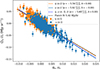 |
Fig. A.1. Reproduction of Planck results with a stellar polarization sample used in Planck Collaboration XII (2020), but using the methodology described in Sect. 3. |
There is a small difference between our derived polarization ratio RP/p = 5.79 (dashed blue line in Fig. A.1) and the value reported by the Planck collaboration, 5.42 (dashed black line). We performed the analysis using the Planck PR3 and the Planck PR4 data. We find minor differences in the derived slopes between the two choices of dataset. In particular, the slope of the Qs − qv relation changes from -5.59±0.19 MJy sr−1 (PR3) to  MJy sr−1 (PR4), that of Us − uv changes from
  MJy sr−1 (PR3) to
  MJy sr−1 (PR4) and the joint fit slope changes from −5.79 ± 0.11 MJy sr−1 to −5.80 ± 0.11 MJy sr−1 (PR4). Systematic uncertainties alone are too small to explain the difference between our best-fit slope and that found by Planck Collaboration XII (2020).
We attribute this difference to several factors. First, unlike Planck Collaboration XII (2020), we have not corrected the stellar Stokes parameters for the background ISM contribution, that is, we have not derived the q∞, u∞ values that estimate the polarization assuming the star is located at infinity. Second, it could be due to our line-of-sight selection, as we did not explicitly exclude sightlines with low E(B − V)★/E(B − V)∞ ratios. Finally, we did not apply a beam depolarization correction to the Planck maps. Despite these differences in methodology, the agreement of our fitted relations shown in Fig. A.1 with the results of Planck Collaboration XII (2020) is remarkably good.
Appendix B: Non-linearity in the Qs–qv relationship
An important aspect of our analysis is the apparent non-linearity in the correlation between the Planck Stokes parameter Qs and the corresponding stellar Stokes parameter qv. A close inspection of the fit presented in Fig. 2 reveals non-linearities in the residuals.
A striking signature of this non-linearity is seen if we mask the middle portion of Qs−qv datasets in Fig. 2. When excluding the central values, the resulting linear fits no longer pass symmetrically through the data: points with large negative qv tend to lie above the fit, while those with large positive qv lie below. This behavior violates the basic expectation from a linear model.
We interpret this non-linearity as a consequence of the varying relative contribution of multiple clouds along the line of sight. When the relative contribution of each cloud changes (e.g., due to a distance cut or sky region selection), the resulting Qs–qv relationship reflects a mix of different effective slopes. The Qs signal depends more heavily on the balance between cloud 1 and cloud 2 contributions than the Us signal, which appears more stable across distance cuts.
This interpretation is further supported by the tomographic decomposition of the stellar polarization data (Pelgrims et al. 2024), which shows that some of the pixels are dominated by a single cloud, and others have an equal contribution from both clouds along the LOS. For instance, we examine how the relative contribution to the stellar qv signal varies across the field using the tomographic decomposition data obtained in Pelgrims et al. (2024). For each pixel, we obtain the mean of the posterior distribution of the Stokes q of each cloud along the LOS. We then compute the absolute ratio  in each pixel, where
  and
and  are the Stokes qv of the first and second cloud along the LOS, respectively. The resulting map (Fig. B.1) reveals strong gradients: in the upper-left portion
  (cloud 2 is weak), whereas in the right part of the map there is a region where the opposite is true as cloud 2 induces 8 times more signal in qv than cloud 1.
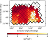 |
Fig. B.1. Map of |

These spatial variations of the relative importance of each cloud are likely the origin of non-linearities in the Qs–qv relation, and are likely also the reason that we find a notable dependence of RQq on the choice of stellar sample. The two samples vary in their properties: the > 450 pc sample has a mean of ∼ 14 stars per pixel, while the > 2000 pc sample has a mean of ∼ 3 stars per pixel. In the > 2000 pc case, two effects act simultaneously: (i) the number of populated pixels falls from 86 to 71 (15 are excluded), with roughly one third of these exclusions occurring in regions where cloud 2 is weak; and (ii) the stellar sampling per pixel becomes much sparser, with the mean decreasing from ∼ 14 to ∼ 3 stars per pixel.
We conclude that the assumption of a single linear relation between Qs and qv may oversimplify the actual astrophysical complexity in this region. While a linear model can still capture an average trend, care must be taken in interpreting the slope as a global physical quantity.
All Tables
All Figures
|
Fig. 1. Gnomonic projections of the pixelized Stokes parameter data at optical (top) and submillimeter (bottom) at Nside = 256 and distance cut > 450 pc. Top left: qv; Top right: uv; Bottom left: Qs; Bottom right: Us. The Stokes parameters follow the IAU convention. Pixels with no optical data (outside of the observed sky region) are white. |
| In the text | |
|
Fig. 2. Correlation between the Stokes parameters from Planck (Qs, Us) and the fractional Stokes parameters from RoboPol (qv, uv). The blue points represent the correlation between Us and uv, while the orange points show the correlation between Qs and qv. The blue dashed line indicates the best-fit line of the joint correlation determined by minimizing χ2, while the solid blue and solid orange lines correspond to the Us − uv and Qs − qv fits, respectively. The black dashed line corresponds to the value from Planck Collaboration XII (2020). |
| In the text | |
|
Fig. 3. Comparison of best-fit slope values for different star sample selections. All cases are analyzed at the same Nside of 256. The slope found in Planck Collaboration XII (2020) is shown as the black dashed line. |
| In the text | |
|
Fig. 4. Distributions of ΔΨs/v (in degrees) for stars with distance d ≥ 2000 pc (left) and d ≥ 450 pc (right). The red vertical lines indicate the distribution’s median; the values are reported in the legend. |
| In the text | |
|
Fig. 5. Correlation plots and linear fits between (Qs, qv) and (Us, uv) for two values of the polarization degree, p = 1.5% (top row) and p = 2.5% (bottom row). Each column corresponds to a combination of magnetic field orientation ΨB⊥ = {30°, 60°} and miscalibration offset β = {3°, 7°}, increasing from left to right. The best-fit values for the slopes (absolute value) and for the intercept obtained for the correlations are given in the legend; the resulting model is shown on the scatter plot, in blue for (Qs, qv) and in orange for (Us, uv). They are expressed in MJy sr−1. To generate the data, we used Rp/p = 5.42 MJy sr−1, σΨB⊥ = 5°, and σp = 0.2% to produce the dynamical range. |
| In the text | |
|
Fig. 6. Correlation plot for the simulated example of two intervening clouds with different polarization properties and different RP/p ratios, as described in the text. |
| In the text | |
|
Fig. A.1. Reproduction of Planck results with a stellar polarization sample used in Planck Collaboration XII (2020), but using the methodology described in Sect. 3. |
| In the text | |
|
Fig. B.1. Map of |
| In the text | |
Current usage metrics show cumulative count of Article Views (full-text article views including HTML views, PDF and ePub downloads, according to the available data) and Abstracts Views on Vision4Press platform.
Data correspond to usage on the plateform after 2015. The current usage metrics is available 48-96 hours after online publication and is updated daily on week days.
Initial download of the metrics may take a while.