| Issue |
A&A
Volume 708, April 2026
|
|
|---|---|---|
| Article Number | A181 | |
| Number of page(s) | 15 | |
| Section | Interstellar and circumstellar matter | |
| DOI | https://doi.org/10.1051/0004-6361/202557833 | |
| Published online | 09 April 2026 | |
A cationic carrier for the diffuse interstellar band at 862.1 nm: Evidence of the skin effect in nearby diffuse to translucent clouds
1
Chinese Academy of Sciences South America Center for Astronomy (CASSACA),
Camino El Observatorio 1515,
Las Condes,
Santiago,
Chile
2
Departamento de Fisica y Astronomia, Facultad de Ciencias Exactas, Universidad Andres Bello,
Fernandez Concha 700,
8320000
Santiago,
Chile
3
Shanghai Astronomical Observatory, Chinese Academy of Sciences,
80 Nandan Road,
Shanghai
200030,
China
★ Corresponding author: This email address is being protected from spambots. You need JavaScript enabled to view it.
Received:
25
October
2025
Accepted:
5
March
2026
Abstract
The tendency of some diffuse interstellar band (DIB) carriers to concentrate in the outer UV-illuminated layers of molecular clouds (MCs), the so-called skin effect, makes their spatial distribution a powerful probe of their physical nature. We leveraged Gaia DR3 measurements of the DIB at 862.1 nm to investigate its behavior across 12 nearby MCs, spanning diffuse to translucent regimes (AV ~ 0.2-3.5 mag). We find significant diversity in the DIB behavior, both between different clouds and within individual clouds from their outer to inner regions. To quantify these trends, we employed a piecewise linear model to fit the average slope (α) between the normalized DIB strength, log10(W8621/AV), and dust extinction, log10(AV). In general, log10(W8621/AV) declines with log10(AV) with α between 0 and −1 and becomes progressively steeper at higher AV. These observed slopes and their variations are consistent with the photoionization equilibrium models, where the carrier abundance is governed by local conditions, particularly the UV radiation field and cloud structure (e.g., density profiles or clumpiness). Particularly, the Taurus cloud region uniquely displays an initial increase in log10(W8621/AV) at low extinction, a signature predicted for a cationic carrier. By fitting the slope of this rising trend, we estimate an ionization potential of EIP = 12.40−2.29+1.90 eV for the DIB λ8621 carrier, which agrees well with the secondary ionization energies of large carbonaceous molecules such as polycyclic aromatic hydrocarbons or fullerenes. Furthermore, by comparing the peak position of log10(W8621/EB-V) in Taurus with other prominent optical DIBs, we propose a spatial sequence within clouds, placing the layer of the λ8621 carrier between the layers of λ5780 and λ6614. Our results support a cationic carrier for DIB λ8621 and help situate it within the broader context of the DIB family.
Key words: ISM: lines and bands
© The Authors 2026
 Open Access article, published by EDP Sciences, under the terms of the Creative Commons Attribution License (https://creativecommons.org/licenses/by/4.0), which permits unrestricted use, distribution, and reproduction in any medium, provided the original work is properly cited.
This article is published in open access under the Subscribe to Open model. This email address is being protected from spambots. You need JavaScript enabled to view it. to support open access publication.
1 Introduction
Diffuse interstellar bands (DIBs) are absorption features that are ubiquitously observed in the interstellar medium (ISM) of the Milky Way (Kos et al. 2014; Zasowski et al. 2015; Gaia Collaboration, Schultheis 2023b), in external galaxies (Cordiner et al. 2011; Monreal-Ibero et al. 2018; van Erp et al. 2025), and in distant quasars (Junkkarinen et al. 2004; York et al. 2006; Lawton et al. 2008). Over 600 DIBs have been confirmed between 0.4 and 2.4 μm (Hobbs et al. 2008, 2009; Cox et al. 2014; Fan et al. 2019; Hamano et al. 2022; Ebenbichler et al. 2022). Despite their ubiquity, the origin and nature of the carriers that cause these weak and broad absorption features have remained a mystery for over a century since their discovery (Heger 1922). Currently, complex carbon-bearing molecules are widely considered the most promising candidates for DIB carriers. This view is supported by the successful laboratory identification of  as the carrier of five DIBs between 9300 and 9700 Å (Campbell et al. 2015; Walker et al. 2016; Linnartz et al. 2020) and by the detection of resolved substructures in the profiles of DIBs λ57971, λ6379, and λ6614 in high-resolution spectra. These substructures provide evidence for unresolved rotational contours arising from the electronic transitions of large molecules (Sarre et al. 1995; Huang & Oka 2015; MacIsaac et al. 2022). Numerous candidates have been proposed, including carbon chains (Maier et al. 2004), polycyclic aromatic hydrocarbons (PAHs; Salama et al. 1996; Ehrenfreund & Foing 1996; Sonnentrucker et al. 1997; Ruiterkamp et al. 2005), fullerenes (Webster 1993; Fulara et al. 1993; Omont 2016), and polyacenes (Omont et al. 2019), but none have yet been definitively confirmed.
In addition to laboratory measurements and high-resolution spectroscopy, another key method for inferring the properties of DIB carriers and constraining their nature is to study the behavior of DIB strengths in different environments relative to known ISM species. A linear relation between dust extinction and the equivalent width (WDIB) of a DIB has been widely reported since the 1930s (e.g., Merrill & Wilson 1938; Friedman et al. 2011; Lan et al. 2015). However, this correlation is often attributed to the general increase in the abundance of all ISM species with distance along a sightline and does not always hold (Krelowski 2018). Observations have indeed revealed different vertical scale heights for dust grains and DIB carriers (Zhao et al. 2023; Lallement et al. 2024). For sightlines probing isolated cloud regions, WDIB is often weaker than expected from the dust extinction, and it eventually stops to grow with increasing cloud opacity, which implies that the majority of DIB carriers are concentrated in the outer cloud layers (Herbig 1995; Snow 2014). This phenomenon is commonly referred to as the skin effect and was first reported by Wampler (1966). Snow & Cohen (1974) systematically studied the skin effect for DIBs λ4428 and λ5780 in the ρ Ophiuchus cloud, followed by reports for other strong optical and near-infrared DIBs (e.g., Meyer & Ulrich 1984; Adamson et al. 1991, 1994; Sonnentrucker et al. 1997; Snow et al. 2002; Vos et al. 2011; Elyajouri & Lallement 2019).
The skin effect is an environmental phenomenon that reflects changes in the life cycle and charge state of DIB carriers as they move from the outer to the inner regions of clouds under varying physical conditions, such as the local ultraviolet (UV) radiation field, temperature, and density. By combining observations of the Orion HII and Taurus-Perseus regions, Sonnentrucker et al. (1997, hereafter S97) observed a two-stage behavior for four optical DIBs: λ5780, λ5797, λ6379, and λ6614. Their normalized strength, log10(WDIB/EB-V), first increased up to EB-V ~ 0.20.3 mag and then began to decrease out to EB-V ~ 1 mag. This two-stage behavior was also noted by Jenniskens et al. (1994) for λ6284 in Orion region. S97 developed a photoionization equilibrium (PIE) model to infer the ionization properties of DIB carriers, assuming a constant electron density and uniform cloud opacity. In their model, the initial increase in log10(WDIB/EB-V) occurs in UV-penetrated regions where the DIB carrier abundance is inversely proportional to the UV flux (ΦUV). The positive slope of the log10(WDIB/EB-V) versus EB-V relation is determined by the dust extinction curve (RV) and the ionization potential (EIP) of the carrier. Deeper within the cloud, at higher EB-V, the carrier abundance decreases as ΦUV drops exponentially with optical depth. The carrier abundance reaches a limit (WDIB becomes constant) when the UV radiation is fully attenuated. This scenario predicts that DIB carriers are concentrated in a specific layer of a cloud and is supported by the observed sensitivity of DIB strengths and profiles to the UV radiation field (Jenniskens et al. 1994; Cami et al. 1997; Vos et al. 2011). Based on their estimated EIP of around 10 eV, Sonnentrucker et al. 1997 proposed ionized PAHs as carriers for DIBs λ5780, λ5797, and λ6614.
Different DIBs are observed to reach their maximum WDIB/EB-V at different EB-V values (Snow & Cohen 1974, S97, Snow et al. 2002), and a given DIB can exhibit different behavior with respect to dust extinction in different clouds (Elyajouri & Lallement 2019). We leverage the large DIB λ8621 catalog from the third data release of Gaia (Gaia DR3; Gaia Collaboration, Vallenari 2023; Gaia Collaboration, Schultheis 2023b) to statistically investigate the variation in its normalized strength, log10(W8621/AV), with respect to dust extinction, log10(AV), in diffuse to translucent regions (AV ~ 0.2-3.5 mag) toward 12 nearby molecular clouds (MCs). Our main goals are 1) to infer the ionization properties of the λ8621 carrier using the S97 PIE model and 2) to quantitatively characterize the dependence of the λ8621 carrier behavior on local environmental conditions. This paper is organized as follows: The DIB catalog, the calculation of AV, and the target selection are described in Sect. 2. Section 3 introduces the model we used to fit the average slopes between log10(AV) and log10(W8621/AV). The results are presented in Sect. 4, and discussions are provided in Sect. 5. Finally, we summarize our main conclusions in Sect. 6.
2 Data and target clouds
2.1 DIB catalog
The Gaia DR3 catalog contains a vast number of DIB λ8621 measurements that were derived from spectra of background stars observed by the Gaia Radial Velocity Spectrometer (RVS; Cropper et al. 2018; Sartoretti et al. 2018, 2023). These measurements were obtained by fitting the DIB profile in residual interstellar spectra. The interstellar spectra were produced by subtracting synthetic stellar templates, generated by the module called general stellar parameterizer from spectroscopy (GSP-Spec) (Recio-Blanco et al. 2023) within the astrophysical parameter inference system (Apsis; Creevey et al. 2023). A detailed description of the fitting procedure, quality control, and validation processes is provided in Zhao et al. (2021a) and Gaia Collaboration, Schultheis (2023b). After removing entries with poor-quality DIB parameters or unreliable stellar templates, Gaia Collaboration, Schultheis (2023b) defined a high-quality (HQ) sample containing approximately 140000 sightlines. However, even this HQ sample has been shown to include biases caused by contamination from nearby Fe I stellar lines (Saydjari et al. 2023; Zhao et al. 2024a). Therefore, we applied a further set of filtering criteria to the HQ sample, as listed below.
The DIB quality flag needs to be zero, which indicates the highest measurement quality (Gaia Collaboration, Schultheis 2023b).
The DIB radial velocity2, expressed in the kinematical local standard of rest, is required to be within ±50 kms−1 as the target clouds are nearby (see e.g., Wakker 1991; Lewis et al. 2022).
Sightlines toward background stars with Teff = 4250 K and log g = 1.5 are excluded to avoid the GSP-Spec parameterization problems encountered for cool stars (see Sect. 8.6 of Recio-Blanco et al. 2023).
The Gaussian width of the DIB profile needs to be greater than 1.2 Å. This threshold is imposed to exclude very narrow features that are likely to be artifacts from the imperfect subtraction of stellar lines, rather than genuine DIB absorption, considering that the spectral resolution of RVS spectra is about 0.75 Å at 8621 Å.
The application of these criteria yielded a clean DIB catalog containing 95 428 sightlines. From this catalog, a subset of 2622 sightlines was selected for the present analysis (see Sect. 2.3 and Table 2). In this subset, 96% of the background stars have Teff > 4000 K, with a minimum temperature of 3719 K.
The measured DIB profiles are primarily contaminated by the residuals of stellar Fe I lines. A precise quantification of the maximum residual for each spectrum is not possible, as the processed DIB spectra are not part of Gaia DR3. In our subsequent work (Gaia Collaboration, Schultheis 2023a; Zhao et al. 2024a), however, we established that the magnitude of these stellar line residuals is strongly dependent on the spectral signal-to-noise ratio (S/N). We found that for spectra with S/N > 50, the residuals are typically within 0.02, whereas they can exceed 0.05 in spectra with lower S/N. In our sample, the median W8621 is 0.17Å. Given a mean Gaussian width of 2Å for λ8621 (Zhao et al. 2024a), this corresponds to a central depth of 0.034 below the normalized continuum. This comparison underscores that DIBs are intrinsically weak features, and the use of derived ISM spectra is essential for the reliable selection of high-quality DIB measurements.
2.2 Dust extinction
We determined the color excess, E(GBP - GRP), for each background star by subtracting its predicted intrinsic color from its observed color (GBP - GRP). The intrinsic color was predicted using an eXtreme Gradient Boosting (XGBoost) model that takes the star’s GSP-Spec atmospheric parameters (effective temperature Teff, surface gravity log g, and metallicity [M/H]) as input. XGBoost is an optimized and scalable tree-boosting library (Chen & Guestrin 2016). As detailed in Zhao et al. (2024b), the model was trained on a sample of dust-free stars using the open-source package xgboost3. The total uncertainty on E(GBP - GRP) was computed by combining three sources of error in quadrature: (1) the photometric errors of the star, (2) the propagated uncertainty from the atmospheric parameters, estimated via a Monte Carlo simulation with 1000 iterations, and (3) the intrinsic model uncertainty. To estimate the model uncertainty for a given star, we first identified its nearest neighbor within the model test set based on the atmospheric parameter space. The residual between the observed (GBP - GRP) and the XGBoost prediction for that test-set neighbor was then adopted as the contribution of the model uncertainty for the target star.
To facilitate a more direct comparison with other studies and provide a more physically intuitive measure of extinction, we converted E(GBP - GRP) into the V-band extinction, AV. This conversion was performed using the standard extinction law from Cardelli et al. (1989), assuming RV = 3.1. We did not account for potential effects from filter bandpass curvature (Wang & Chen 2019; Maíz Apellániz 2024) or variations in RV. This simplification is justified because our analysis focuses on diffuse and translucent interstellar clouds, where extinction values are generally not high (AV ≲ 3.5 mag) and RV is not expected to vary significantly. A detailed investigation of the effect of the RV variation is deferred to a future paper.
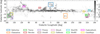 |
Fig. 1 Location of target cloud regions (colored rectangles with names marked below), overplotted on 12CO (J = 1-0) intensity map from Dame et al. (2001). |
2.3 Target selection
We investigated the behavior of the DIB λ8621 in the transition from diffuse to translucent interstellar environments (AV ~ 0.23.5 mag; Snow & McCall 2006). Our analysis targeted 12 nearby MCs. The Galactic longitude and latitude (l/b) boundaries for these regions were adapted from Lee et al. (2018) and Lewis et al. (2022), with minor adjustments made for this study. The cloud distances (dMC) were adopted from the references within those works. For simplicity, we refer to these target regions by their conventional MC names. A map showing the sky locations of these regions is presented in Fig. 1, and their properties are summarized in Table 1. These specific clouds were chosen because their relative isolation minimizes contamination from unrelated foreground and background interstellar material along the line of sight.
To probe the dust extinction and DIB absorption within these clouds, we selected background stars that satisfied several criteria. First, a star must be located on the sky within the defined l/b boundaries of a target cloud and have a geometric distance (Bailer-Jones et al. 2021) between dMC + 100 pc and 1500 pc to ensure that it lies behind the cloud. Second, to ensure a high-quality dataset, we imposed further constraints: the relative uncertainty on the stellar distance and the DIB W8621 must be lower than 20%. Finally, to ensure robust detections, we required W8621 > 0.02 Å and AV > 0.2 mag. The final number of selected sightlines for each cloud is listed in Table 2, and their spatial distributions are illustrated in Fig. A.1. This figure shows that the very densest regions of the MCs remain largely unprobed, an observational bias resulting from high extinction combined with the limiting magnitude of the Gaia RVS instrument. As demonstrated in Fig. 2, the skin effect is evident in all target clouds. The median trends (blue squares) clearly reveal a diversity in the DIB-to-dust relation among different clouds and across the diffuse-to-translucent transition within individual clouds.
Investigated cloud regions sorted by their distances.
3 Method
The relation between log10(W8621/AV) and log10(AV) is often complex and cannot be adequately described by a single linear model. The observed trend frequently exhibits changes in slope, which are indicative of shifts in the underlying physical or chemical processes, such as a transition from a growth phase to one of saturation or destruction in denser regions of a cloud. To quantitatively characterize these transitions without presupposing a specific complex physical model, we employed a piecewise linear model (PLM). While the true relation is likely continuous and nonlinear, the PLM provides a robust method for approximating the average slope within distinct extinction regimes. These fitted slopes can then be used to compare the DIB skin effect in different clouds and to infer the effect of environmental conditions on the properties of the DIB carrier.
Results of the selected PLM for each cloud.
3.1 Piecewise linear model (PLM)
The fundamental idea of the PLM is to approximate the continuous curved relation in log-log space with a series of connected straight-line segments. Each linear segment corresponds to a distinct regime in which the relation between W8621/AV and AV can be approximated by a single power law. The connection points between segments, referred to as knots, represent the transitional extinction values at which the nature of this relation changes. The PLM is a continuous function whose slope changes at these discrete knots. For a model with n linear segments defined by n - 1 knots, the function is expressed as
 (1)
(1)
where x = log10(AV) and f(x) = log10(W8621/AV). C is the intercept of the first linear segment. α1 is the slope of the initial segment, valid for x < k1. ki is the position of the ith knot along the x-axis, with the knots ordered such that k1 < k2 < ∙ ∙ ∙ < kn−1. Each knot represents a transitional log10(AV) value. ∆αi is the change in the slope at knot ki. The slope of the (i + 1)th segment (between knots ki and ki+1) is the cumulative sum of all preceding slope changes:  .
.  is the Heaviside step function, defined as 0 for x < ki and 1 for x ≥ ki.
The PLM serves as a powerful empirical tool for analyzing trends in the data. However, it is important to recognize its inherent assumptions. The model approximates a potentially smooth continuous curve with discrete transitions at the knots. In physical reality, these transitions are likely more gradual. Therefore, the knots should be interpreted not as precise physical thresholds, but as the characteristic extinction values around which the dominant physical regime changes. Similarly, the linearity of each segment is an approximation of the true relation within that regime.
3.2 Fitting procedure
A key challenge in applying a PLM is selecting the appropriate number of linear components (np). A model with too few components may fail to capture significant trends in the data, while a model with too many free parameters risks overfitting, where it begins to model random statistical noise instead of the underlying physical relation. To balance model complexity and goodness-of-fit, we adopted a systematic approach. For each target cloud, we fit a series of PLMs with an increasing number of components (np = 1-4) and then selected the optimal model by visual inspection. This ensured that our final results reflect genuine large-scale changes in the DIB behavior.
For our fitting procedure, the model with np components was parameterized directly by {C, α1, ∆αi, ki}, where i ranged from 1 to np - 1. This parameterization, which models the changes in slope (∆ai) at each knot, is often more statistically robust and leads to a more efficient sampling of the parameter space compared to fitting the absolute slopes directly. We assigned uniform priors to the model parameters. The specific ranges were C ∈ [0,5], α1 ∈ [−5,5], and ∆αi ∈ [−15,15]. The priors for the knot locations, ki, were also uniform, constrained to lie within the observed range of log10(AV) for each cloud, and ordered such that k1 < k2 < ∙ ∙ ∙ < knp-1.
To properly account for observational uncertainties in log10(AV) and log10(W8621/AV), we constructed a likelihood function following the method of Li et al. (2020). The total likelihood for a set of N data points D = {xi, yi} given a model prediction M = {xm, ym} is the product of the individual probabilities,
 (2)
(2)
![Mathematical equation: \begin{align} P(D_i|M) &= \frac{1}{2\pi\sigma_{x_i}\sigma_{y_i}} \exp\left[-\frac{1}{2}\left( \frac{(x_i - x_m)^2}{\sigma_{x_i}^2} + \frac{(y_i - y_m)^2}{\sigma_{y_i}^2} \right)\right], \end{align}](/articles/aa/full_html/2026/04/aa57833-25/aa57833-25-eq42.png) (3)
(3)
where the uncertainties σx and σy on the logarithmic quantities were derived from the observational errors via standard error propagation,
 (4)
(4)
![Mathematical equation: \sigma_y &= \frac{1}{\ln(10)}\left( \left[\frac{\sigma(\Wgaia)}{\Wgaia}\right]^2 + \left[\frac{\sigma(\Av)}{\Av}\right]^2\right)^{1/2}.](/articles/aa/full_html/2026/04/aa57833-25/aa57833-25-eq44.png) (5)
(5)
The posterior probability distributions for the model parameters were sampled using the nested sampling algorithm (Skilling 2004), as implemented in the Python package dynesty (Speagle 2020). From the resulting posterior distributions, the best-fit value for each parameter was taken as the median (50th percentile), and the uncertainties were defined by the 16th and 84th percentiles, which enclose a 68% (1σ) confidence interval.
While the model was fit using the slope changes, ∆αi, the absolute slopes of each segment, αi, are more physically intuitive. Therefore, for our final analysis and reporting in Tables 2 and B.1, we calculated the absolute slopes from the posterior samples using the relation  . This allowed us to directly assess the DIB behavior in each regime, such as identifying the onset of saturation where the slope approaches a value of α = −1.
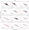 |
Fig. 2 Variation in log10(W8621/AV) as a function of log10(AV) for each target cloud. The corresponding AV scale is shown at the top of each panel. The points are color-coded by their number density, estimated via a Gaussian KDE. The blue squares represent the median log10(W8621/AV) in bins of log10(AV) (from −0.8 to 0.6 with a step of 0.1). The solid red line and shaded region show the selected PLM and its 99.7% credible interval, respectively. The vertical dashed orange lines indicate the knot locations (see Sect. 3.1). The full PLM fitting results with np = 1−4 for each cloud can be found in Fig. B.1. For Cepheus South, the points marked with black crosses were clipped as outliers and excluded from the fit (see Sect. 4 for details). Each panel is labeled with the cloud name, distance, and the number of sightlines. |
4 Results
The full PLM fitting results for all target clouds, testing models with np = 1 to 4 components, are presented in Fig. B.1. The complete set of derived parameters for every tested model is listed in Table B.1.
For each cloud, we selected the optimal model from the set (np = 1-4) based on visual inspection, considering the physical plausibility of the resulting parameters. First, we avoided PLMs with unrealistically hgih α values (e.g., α2 in the np = 3 model for Ophiuchus), which imply an abrupt change in the variation of log10(W8621/AV) that cannot be reliably represented by a PLM and would distort the fitting of other slopes. Second, for clouds with fewer data points (e.g., Hercules), the fitting results are more sensitive to scatter. In these cases, we adopted simpler and more stable PLMs with smaller np to minimize overfitting. The selected PLM for each cloud is shown in Fig. 2, with the corresponding parameters listed in Table 2. A brief summary of the model selection for each cloud is provided below.
Ophiuchus, Chamaeleon, Orion B, and California: These four clouds exhibited a similar behavior. While models with np > 2 were tested, the more complex models tended to introduce abrupt high-magnitude slope changes to accommodate minor scatter, which was not statistically justified. We therefore conservatively selected the np = 2 model for all four, characterizing the trend as a simple break.
Taurus is the only cloud in our sample for which the median trend suggests an initial ascent in log10(W8621/AV) at low AV, consistent with the predictions of S97. However, due to the small number of data points in this regime (AV ≲ 0.6 mag), the PLM fit was unable to robustly capture this feature. A test fit required np ≥ 8 to model the ascent, which is an unjustifiably complex model that constitutes severe overfitting. We selected np = 2 to describe the dominant trend of decreasing log10(W8621/AV) after its peak.
Hercules has the lowest line-of-sight dust column in our sample (AV ~ 1 mag) and exhibits significant scatter. Although a few points at AV < 0.3 mag have a lower log10(W8621/AV), the data are too sparse to confirm a distinct trend. We selected the singlecomponent model (np = 1) as adding more components would merely have meant fitting noise.
Perseus: For AV > 1.5 mag, a distinct flattening end is evident in the median trend and the models with np ≥ 2. This suggests a potential re-increase in WDIB with AV in dense regions. This is a newly observed phenomenon. We finally selected the np = 3 model because it captured the behavior in low- and high-extinction regimes best, matched to the median trend, although the data in these regime are limited to a small number of sightlines with large scatter. The fit reveals three distinct regimes: An initial decline with slope  for AV ≲ 1 mag, a dramatically steeper drop with
  between AV ≈ 1−1.5 mag, and a flattening to a nearly zero slope (
 ) for AV > 1.5 mag.
Orion A: a simple linear model (np = 1) was sufficient to describe the trend in Orion A, yielding a continuous decrease with slope  . While the median trend appears to be flatter for AV < 0.8 mag, the PLM fit, which accounts for all individual data points and their uncertainties, found no statistical support for a break. The np = 3 model for Orion A (see Fig. B.1) deviates significantly between the median model line and the credible region. This is a clear sign of a poorly constrained and not robust fit.
Mon OB1: for this cloud, the simple np = 1 model failed to capture the global trend, while models with np > 1 primarily used the additional components to fit scattered points at AV > 1.5 mag. The np = 2 model was statistically preferred, but the second slope, α2, was poorly constrained. Therefore, we selected the np = 2 model but only consider the first slope,  , to be a physically robust result.
Mon R2: Similar to Perseus, Mon R2 exhibits a plateau after an initial decline. The trend is best described by the np = 2 model, with a steep initial slope of  followed by a flat second segment where
  .
.
Cepheus South: initial fits to this cloud failed for all tested np values. The failure was driven by two outlier data points at log10(AV) ~ 0.2 and log10(W8621/AV) ~ 1.8, which had very low reported uncertainties and thus affected the fit strongly. As this was the only cloud where all tested fits failed, we took the exceptional step of applying an outlier-clipping procedure based on a Gaussian kernel density estimation (five clipped points are marked by black crosses in Figs. 2 and B.1). After clipping, the data were well described by an np = 2 model. We refrained from applying this clipping to other clouds as scattered points might contain real physical information.
Canis Major: The np = 2 model was selected. It describes a trend that begins with a much flatter slope ( ) and then steepens to
  .
.
Our model selection indicates a clear preference for simpler models, constrained by observational scatter and inherent model limitations. Eight clouds are best described by a two-component model (np = 2), three clouds4 are best described by a singlecomponent model (np = 1), and only cloud, Perseus, required a three-component model (np = 3). A comparison of the fitted slopes and knot locations for the selected models is presented in Fig. 3. Most initial slopes (α1; blue hexagons) fall between 0 and −1, indicating a general decline of log10(W8621/AV) with respect to log10(AV) as sightlines probe from diffuse to translucent regions. Clouds fitted with an np = 2 model typically exhibit a steepening trend, where the slope transitions from a shallower value (−1 <α1 < 0) in the outer regions to a steeper one (α2 ≲ -1) in the inner regions. This is qualitatively consistent with the predictions of the S97 PIE model. Two notable exceptions deviate from this simple steepening pattern: Perseus and Mon R2 display a distinct flattening of the slope (α ≈ 0) in their densest regions (AV ≳ 1.5 mag). This feature is not explicitly predicted by the PIE model.
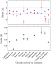 |
Fig. 3 Comparison of the slopes and knots of the selected PLM between target clouds. The slopes are arranged with increasing log10(AV) and are marked with different colors. |
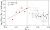 |
Fig. 4 Linear fit to the relation between log10(W8621/EB-V) and EB-V for sightlines in the Taurus cloud with EB-V < 0.2 mag. The data points included in the fit are shown as red squares. The best-fit line is shown in red, and the resulting slope (αT) and the Pearson correlation coefficient (rp) are indicated. |
5 Discussion
5.1 Taurus region and carrier ionization properties
Of the clouds in our sample, Taurus alone exhibits a clear ascending trend of log10(W8621/AV) at low extinction (AV ≲ 0.6 mag). This behavior is predicted by the S97 PIE model for an ionized carrier. This makes it an excellent target for studying the properties of the DIB λ8621 carrier within the framework of the PIE model. This trend is not seen in other target clouds, although they also contain sightlines with low extinction. As the increase in log10(W8621/AV) occurs in the UV-penetrated regions, a possible explanation is that sightlines with strong UV radiation are not probed for these clouds. The ascending trend was seen in Orion region for DIB λ6284 by Jenniskens et al. (1994), but their background stars are not contained in our sample.
By simplifying the relation between WDIB and optical depth and considering a homogeneous diffuse region, we express the positive slope in Taurus as  (Eq. (8) in S97). We performed a linear fit to the sightlines in Taurus with EB-V < 0.2 mag and obtained a slope of
  , and the uncertainties were estimated via Monte Carlo resampling (shown in Fig. 4). Within the PIE model, the value of αT depends on the characteristic wavelength of the ambient UV radiation field that ionize the DIB carriers. For a given RV, this allows us to determine the corresponding photon energy (hν), which is interpreted as the EIP of the carrier. Figure 5 illustrates the theoretical dependence of αT on EIP for several values of RV. Our measured αT corresponds to an ionization potential of
  eV for the λ8621 carrier when applying RV = 3.1. The EIP uncertainty is simply estimated by the fitting error of αT. Our calculations of this relation are consistent with those presented in S97 (their Table 2); minor differences arise from our use of the Cardelli et al. (1989) extinction curve versus the Savage et al. (1977) curve used in their study. An EIP of ~12eV is compatible with the known second ionization potentials of PAHs (Malloci et al. 2007; Holm et al. 2011) and fullerenes (e.g., C20-C70; Díaz-Tendero et al. 2006). This suggests that the λ8621 carrier might be a singly charged PAH or fullerene cation, an inference analogous to that drawn by S97 for the optical DIBs λ5780, λ5797, and λ6614.
The skin effect shows that DIB carriers are most abundant in the outer UV-illuminated layer of clouds. Consequently, the relative distribution of different DIBs as a function of cloud opacity (a concept known as the spatial sequence) is a key diagnostic for investigating carrier properties. S97 argued that a DIB whose normalized strength (WDIB/EB-V) peaks at a lower value of EB-V must have a carrier that is more resistant to the stronger UV radiation field in diffuse environments. This framework establishes a sequence of DIBs from those favoring diffuse regions to those favoring denser, more shielded regions: λ5780 → λ6614 → λ5797 → λ6379. This ordering is consistent with sequences derived from other diagnostics, such as the tightness of the correlation between WDIB and HI column density (Friedman et al. 2011) and the peak in WDIB/EB-V relative to the molecular hydrogen fraction (Fan et al. 2017), although these latter studies did not include λ6379.
Our results for DIB λ8621, which peaks at EB-V ~ 0.2 mag in Taurus (see Fig. 4), place it between λ5780 and λ6614 in this spatial sequence. This placement suggests that λ8621 behaves as a σ-type DIB, which are known to correlate well with λ5780, a finding consistent with the suggestion by Wallerstein et al. (2007). Interestingly, this spatial sequence is also consistent with the descending order of their average WDIB/EB-V measured along sightlines toward field stars (Fan et al. 2019): W5780/EB-V > W8621/EB-V > W6614/EB-V > W5797/EB-V > W6379/EB-V. This consistency supports the physical picture in which carriers more stable against UV photons (e.g., the λ5780 carrier) exhibit higher relative strengths in low-density, high-UV environments than less stable carriers (e.g., the λ5797 carrier), which are more rapidly destroyed in such conditions (Krelowski & Westerlund 1988; Herbig 1995; Cami et al. 1997; Vos et al. 2011). Furthermore, this sequence might also relate to carrier size. An analysis of DIB profile substructures by MacIsaac et al. (2022) estimated an increasing carrier size (in number of carbon atoms) along the sequence λ6614 < λ5797 < λ6379, assuming linear or spherical molecules. Taken together, these converging lines of evidence underscore that the behavior of DIBs as a function of dust extinction is a powerful diagnostic tool for exploring the physical and chemical nature of their carriers.
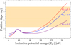 |
Fig. 5 Theoretical relation between the ionization potential (EIP) of a DIB carrier and the expected observational slope (αT) from the PIE model of S97. The relation is plotted for three different RV = 3.1,4.0, and 5.5. The vertical orange line and shaded region represent our measured value of αT for DIB λ8621 (from Fig. 4) and its 1σ uncertainty, respectively. The intersection of our measurement with the RV = 3.1 curve implies EIP ≈ 12 eV. |
5.2 Implications of environmental conditions in different clouds
In nearly all the clouds we investigated, the normalized DIB strength, log10(W8621/AV), decreases with increasing extinction, log10(AV), exhibiting an average slope (α1) between 0 and −1. In addition to Taurus, Hercules is another exception, showing a flatter stage at AV ~ 0.3 mag before steepening. This negative slope in this log-log plot signifies that while W8621 increases as sightlines probe deeper into a cloud, it does so at a slower rate than AV. According to the S97 PIE model, the abundance of an ionized carrier is proportional to the local ΦUV and should therefore decrease exponentially as the UV field is attenuated deeper inside a cloud. To explain the observed net increase in W8621 (even though it is slower than AV), at least two effects must be considered. First, the accumulation of gas toward the cloud center increases the reservoir of neutral precursor molecules available for ionization. Second, the cloud geometry plays a role; for instance, in a simple spherical model, the length of the line-of-sight path through the carrier-bearing region increases toward the cloud center, boosting the total column density to which W8621 is proportional.
The variation in the slope α1 among different clouds likely reflects differences in their internal structures, such as their gas and dust density profiles. A more rapid accumulation of dust, for example, would lead to faster UV attenuation, and thus, to a more negative (steeper) slope α1. This decline continues until a critical extinction, AV, is reached, at which point the slope approaches −1. In the log-log representation of this work, a slope of −1 implies that W8621 has become constant, regardless of any further increase in AV. The physical interpretation within the PIE model is that at AV > AV, the internal UV field is so strongly attenuated that the DIB carrier is no longer produced. Our observations reveal that AV varies significantly among clouds. For the Hercules and Mon R2 clouds, their α1 approaches a value of −1, which implies a low AV of 0.4-0.5 mag. In contrast, the slopes for Ophiuchus, Orion A, California, and Mon OB1 remain greater than −1 (i.e., shallower) even at AV ~ 2−3 mag. The slopes of other clouds decrease from a value between 0 and −1 to below −1, and this transition occurs at a AV of approximately 1-2 mag. This range is characteristic of the translucent-to-dense cloud regime (Snow & McCall 2006).
While the strength of the UV radiation field certainly affects the depth to which carriers can survive, it is likely insufficient on its own to explain this wide range of AV. The local electron density (Ne), which is nearly constant in a diffuse region and starts to drop sharply in the transition from diffuse to translucent gas (Neufeld et al. 2005; Snow & McCall 2006), is another key factor. A lower Ne reduces the carrier-electron recombination rate, which would counteract the effect of UV attenuation and lead to a shallower slope (larger α), thereby increasing AV. This hypothesis can be tested when the estimation of Ne is available for enough sightlines.
Furthermore, the clumpy nonuniform nature of MCs, as revealed by 3D dust maps (e.g., Lallement et al. 2019; Rezaei Kh. et al. 2020; Dharmawardena et al. 2022), is also thought to contribute to the observed variation in AV. To investigate this, we used the 3D dust maps from Lallement et al. (2022, hereafter L22)5 and Edenhofer et al. (2024, hereafter E24)6 to identify and count the number of the principal dust components along the sightline to each background star. For a given sightline, we identified overdensities in the dust profile using the find_peaks function within the scipy package. To account for the resolution and uncertainties of the maps, we defined a peak as a feature with a density exceeding 0.3 mag per kpc and a width of at least 3 pc. The total number of components identified in front of a background star is denoted as Npeaks. The upper panel of Fig. 6 presents an illustrative example for the sightline toward (l, b) = (216.9°, −18.6°) in Orion A, with a background star at a distance of 936 pc. The two dust maps reveal broadly consistent primary dust components along this sightline, although minor discrepancies exist due to their distinct reconstruction methods, underlying datasets, and modeling assumptions. For instance, while both maps detect two dust components between 400 and 500 pc, two separate components between 700 and 800 pc resolved in the L22 map were treated as a single broad component in the E24 map, which additionally identified a component within 200 pc. In general, the L22 and E24 maps yield consistent values for Npeaks. As shown in the lower panel of Fig. 6, the Npeaks values derived from the two maps agree to within ±1 for 74% of sightlines. Larger discrepancies typically arise when broad dust structures are resolved into a different number of narrower components by each map or from differences in the modeled density profiles at larger distances.
Although the investigated sightlines often traverse multiple clouds (see Fig. 7), the velocity cut applied in our selection criteria limits the velocity separation between individual DIB components to be within 50 km s−1. This velocity difference corresponds to a maximum wavelength separation of approximately 1.4 Å between the centers of the DIB profiles originating in different clouds, which is smaller than the intrinsic Gaussian width of the λ8621 profile (Zhao et al. 2024a) and approximately twice the spectral resolution of the GAIA RVS spectra. Consequently, while the presence of multiple components will broaden the observed profile, the total W8621 derived from the single Gaussian fit employed in Gaia Collaboration, Schultheis (2023b) is expected to be affected only very little.
Figure 7 displays the distribution of Npeaks for all investigated sightlines within each target cloud as derived from the E24 map. Clouds with higher values of Npeaks tend to exhibit a larger  . For instance, in the Hercules and Mon R2 clouds, where
  mag, Npeaks is predominantly lower than 4. In contrast, the Ophiuchus, Orion A, and California clouds, which are characterized by AV > 2 mag, include a significant number of sightlines with Npeaks > 5. This observed contribution of Npeaks to the variation in AV can be explained by a model in which a high line-of-sight AV may result from the summation of many lower-density clumps rather than a single dense core. In such a scenario, UV radiation can penetrate the inter-clump medium more effectively, allowing DIB carriers to persist to a greater total column density than would be expected in a homogeneous cloud, resulting in a larger AVV . However, this trend is not universal, indicating that ACV is not solely determined by the clumpy structure of the cloud. A notable exception is Orion B, which exhibits a greater number of peaks than Orion A, but smaller ACV.
The projection of multiple structures along the sightline would also contribute to the scatter in the log10(AV)-log10(W8621/AV) relations. A distinct trend within the Npeaks distribution is evident for the Ophiuchus, Chamaeleon, and California clouds (see Fig. 7): for a given AV, sightlines with larger Npeaks tend to exhibit a larger log10(W8621/AV). Furthermore, when considering clouds with np = 2, α2 increases across the sequence of clouds: Cepheus South, Taurus, Orion B, Ophiuchus, and California. This trend agrees with the increasing prevalence of sightlines with high Npeaks values observed in these same clouds. This finding is consistent with the suggestion by Elyajouri & Lallement (2019), who proposed that a greater number of components along a sightline can flatten the observed trend, thereby yielding a higher value of α, although in the regions they investigated, Cepheus exhibited more complex structures than Orion and Taurus7. Conversely, some clouds deviate from this pattern. Based on their relatively simple structures (predominantly Npeaks ≤ 3), Canis Major and Chamaeleon were expected to have very low α2 values, corresponding to a steep trend. However, their measured α2 values are intermediate, falling between those of Taurus and Orion B.
Several clouds in our sample (Chamaeleon, Taurus, Perseus, Cepheus South, and Canis Major) exhibit regions in which the slope is steeper than −1 (α< −1). This indicates that W8621 decreases actively with increasing AV, a behavior that might be caused by the depletion of carrier molecules onto the surfaces of dust grains or by geometric effects, such as a decreasing effective path length through the carrier-rich region of the cloud. Perseus shows a particularly steep slope (α2) that subsequently transitions to a plateau (α3 ≈ 0) for AV ≳ 1.5 mag. A similar but more poorly sampled flattening is observed in Mon R2. A zero slope in the log10(W8621/AV)-log10(AV) plane corresponds to a linear correlation between W8621 and AV, a trend often seen over large distance ranges through the diffuse ISM (e.g., Munari et al. 2008; Zhao et al. 2021a,b). The structure along sightlines toward Perseus is highly uniform and is mostly characterized by Npeaks = 2. Crucially, these two dust components do not indicate internal clumps within Perseus; one component originates from the Perseus cloud itself, while the other is associated with the wall of the Local Bubble. Thus, the reemergence of this linear trend at high AV cannot be attributed to cloud clumpiness. At present, we only observe this behavior in Perseus and Mon R2 at AV ~ 3 mag, and these detections are based on a small number of sightlines with significant scatter. Further observations probing more sightlines deeper into clouds are needed to confirm whether this repeated increase in the DIB strength is a genuine astrophysical effect, to assess its prevalence, and ultimately, to chart the evolution of DIBs in dense environments.
In summary, the observed behavior of the DIB λ8621 is broadly consistent with the predictions of the S97 PIE model, but the details are modulated by a combination of factors. The variation in the slope α within a single cloud and between different clouds depends not only on the UV field and electron density, but also critically depends on the geometry of the clouds, including their large-scale density profiles and smallscale clumpy substructures. Future investigations focusing on nearby structurally simple clouds (using high-resolution archival spectra of early-type stars capable of resolving individual DIB components and probing denser regions) will be invaluable for disentangling these effects and further constraining the properties of DIB carriers. Ultimately, a comprehensive understanding of these relations could allow the variation of WDIB with AV to be used as a powerful tracer of the UV radiation field and cloud structure in the diffuse and translucent ISM.
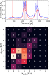 |
Fig. 6 Upper panel : normalized dust density profiles toward the sightline of (l, b) = (216.9°,−18.6°) in Orion A (432 pc), with a background star at 936 pc. The profiles are derived from the dust maps of Lallement et al. (2022, L22, blue) and Edenhofer et al. (2024, E24, red). The dashed vertical lines indicate the detected dust components. Lower panel: the heatmap of the number of the detected dust components (Npeaks) for the 67 sightlines in Orion A derived with the dust maps of L22 and E24. The color scale and numbers represent that both maps detect a specific number of Npeaks (e.g., 6 sightlines have Npeaks = 4 in L22 and E24). |
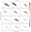 |
Fig. 7 Variation in log10(W8621/AV) as a function of log10(AV) for each target cloud, color-coded by Npeaks of each sightline derived from the E24 map. |
6 Summary and conclusions
With measurements of DIB λ8621 from Gaia DR3 and AV derived from GSP-Spec stellar parameters, we have investigated the variation in the normalized DIB strength, log10(W8621/AV), as a function of extinction, log10(AV), toward 12 nearby molecular clouds, spanning diffuse to translucent regions (AV ~ 0.2−3.5 mag). Our analysis revealed significant diversity in the DIB behavior from one cloud to the next and from the outer to the inner regions of a single cloud. We modeled these trends using a PLM, fitting the average slope (α) of the log10(W8621/AV)-log10(AV) relation over different extinction ranges and selecting the optimal number of segments for each cloud.
For most clouds we investigated, the relation between log10(W8621/AV) and log10(AV) shows an initial decline with an average slope between 0 and −1. This trend reflects a balance between the accumulation of precursor gas and the attenuation of the interstellar UV field with increasing cloud depth. The observed diversity and variation in slopes can be attributed to several key environmental factors that we list below:
The ambient UV radiation field dictates the photoionization equilibrium of the DIB carrier. As dust accumulates deeper inside a cloud, the UV field is attenuated, causing the carrier abundance to drop. When the UV field is effectively extinguished, W8621 becomes nearly constant, and the slope α approaches −1. The critical extinction (AV) at which this occurs varies widely among clouds, from ~0.4 mag (e.g., Hercules) to >3 mag (e.g., Orion A);
The cloud geometry, including the gas and dust density profiles and the presence of clumpy substructures, affects the rate of the UV attenuation, the length of the effective line-of-sight path, and the relation between total column density and local volume density for DIB carriers and dust grains. A longer path length or projection effects from multiple clumps can increase the total carrier column density (and thus, W8621), resulting in a shallower slope. Clumpiness also contributes to the variation in
 and the scatter in the log10(AV)-log10(W8621/AV) relation;
The electron density (Ne), which decreases significantly in the transition to translucent gas, affects the recombination rate of the ionized carrier. A lower Ne reduces the recombination efficiency, allowing the carrier to survive to greater depths, and thus, leading to a shallower slope;
The depletion of carrier molecules onto dust grain surfaces is a potential explanation for clouds exhibiting slopes steeper than −1 (α < −1), such as Taurus and Cepheus South, where W8621 actively decreases with AV.
Taurus alone in our sample shows an initially rising trend of log10(W8621/EB-V) at low extinction (EB-V < 0.2 mag), as predicted by the PIE model for an ionized carrier. A linear fit to this trend yielded a slope of  . For RV = 3.1, this slope corresponds to an ionization potential of
  eV for the DIB λ8621 carrier. This value is consistent with the secondary ionization energies of large molecules such as PAHs and fullerenes. This finding supports the interpretation that the λ8621 carrier is likely a cation, similar to the proposed nature of the optical DIBs at λ5780, λ5797, and λ6614 in S97.
By characterizing the EB-V at which log10(W8621/EB-V) peaks in Taurus and comparing this with the results for other DIBs from S97, we proposed a spatial sequence of DIBs from the outer to the inner regions of a cloud: λ5780 → λ8621 → λ6614 → λ5797 → λ6379. This sequence agrees with their decreasing normalized WDIB reported in Fan et al. (2019).
Together, these results demonstrate that the relation between DIB λ8621 and dust extinction provides powerful constraints on the properties of its carrier and serves as a sensitive probe of cloud structure and local physical conditions. Furthermore, the comparison of the relative behaviors of different DIBs across opacity regimes emerges as a promising avenue for unraveling their shared and distinct characteristics.
Acknowledgements
We thank the referee for a comprehensive review and insightful feedback, which included constructive suggestions that helped to reinforce our results. H.Z. acknowledges financial support by the Chilean Government-ESO Joint Committee (Comité Mixto ESO-Chile) through project No. annlang23003-es-cl. L.Li thanks the support of Natural Science Foundation of China No. 12303026 and the Young Data Scientist Project of the National Astronomical Data Center. This work has made use of data from the European Space Agency (ESA) mission Gaia (https://www.cosmos.esa.int/gaia), processed by the Gaia Data Processing and Analysis Consortium (DPAC, https://www.cosmos.esa.int/web/gaia/dpac/consortium). Funding for the DPAC has been provided by national institutions, in particular, the institutions participating in the Gaia Multilateral Agreement.
References
- Adamson, A. J., Kerr, T. H., Whittet, D. C. B., & Duley, W. W. 1994, MNRAS, 268, 705 [NASA ADS] [CrossRef] [Google Scholar]
- Adamson, A. J., Whittet, D. C. B., & Duley, W. W. 1991, MNRAS, 252, 234 [NASA ADS] [CrossRef] [Google Scholar]
- Bailer-Jones, C. A. L., Rybizki, J., Fouesneau, M., Demleitner, M., & Andrae, R. 2021, AJ, 161, 147 [Google Scholar]
- Boulanger, F., Bronfman, L., Dame, T. M., & Thaddeus, P. 1998, A&A, 332, 273 [NASA ADS] [Google Scholar]
- Cami, J., Sonnentrucker, P., Ehrenfreund, P., & Foing, B. H. 1997, A&A, 326, 822 [NASA ADS] [Google Scholar]
- Campbell, E. K., Holz, M., Gerlich, D., & Maier, J. P. 2015, Nature, 523, 322 [NASA ADS] [CrossRef] [Google Scholar]
- Cardelli, J. A., Clayton, G. C., & Mathis, J. S. 1989, ApJ, 345, 245 [Google Scholar]
- Chen, T., & Guestrin, C. 2016, in Proceedings of the 22nd ACM SIGKDD International Conference on Knowledge Discovery and Data Mining, KDD ’16 (New York, NY, USA: Association for Computing Machinery), 785 [Google Scholar]
- Cordiner, M. A., Cox, N. L. J., Evans, C. J., et al. 2011, ApJ, 726, 39 [NASA ADS] [CrossRef] [Google Scholar]
- Cox, N. L. J., Cami, J., Kaper, L., et al. 2014, A&A, 569, A117 [NASA ADS] [CrossRef] [EDP Sciences] [Google Scholar]
- Creevey, O. L., Sordo, R., Pailler, F., et al. 2023, A&A, 674, A26 [NASA ADS] [CrossRef] [EDP Sciences] [Google Scholar]
- Cropper, M., Katz, D., Sartoretti, P., et al. 2018, A&A, 616, A5 [NASA ADS] [CrossRef] [EDP Sciences] [Google Scholar]
- Dame, T. M., Hartmann, D., & Thaddeus, P. 2001, ApJ, 547, 792 [Google Scholar]
- Dharmawardena, T. E., Bailer-Jones, C. A. L., Fouesneau, M., & ForemanMackey, D. 2022, A&A, 658, A166 [NASA ADS] [CrossRef] [EDP Sciences] [Google Scholar]
- Díaz-Tendero, S., Sánchez, G., Alcamí, M., & Martín, F. 2006, Int. J. Mass Spectrom., 252, 252 [Google Scholar]
- Ebenbichler, A., Postel, A., Przybilla, N., et al. 2022, A&A, 662, A81 [NASA ADS] [CrossRef] [EDP Sciences] [Google Scholar]
- Edenhofer, G., Zucker, C., Frank, P., et al. 2024, A&A, 685, A82 [NASA ADS] [CrossRef] [EDP Sciences] [Google Scholar]
- Ehrenfreund, P., & Foing, B. H. 1996, A&A, 307, L25 [NASA ADS] [Google Scholar]
- Elyajouri, M., & Lallement, R. 2019, A&A, 628, A67 [NASA ADS] [CrossRef] [EDP Sciences] [Google Scholar]
- Fan, H., Welty, D. E., York, D. G., et al. 2017, ApJ, 850, 194 [NASA ADS] [CrossRef] [Google Scholar]
- Fan, H., Hobbs, L. M., Dahlstrom, J. A., et al. 2019, ApJ, 878, 151 [NASA ADS] [CrossRef] [Google Scholar]
- Friedman, S. D., York, D. G., McCall, B. J., et al. 2011, ApJ, 727, 33 [NASA ADS] [CrossRef] [Google Scholar]
- Fulara, J., Jakobi, M., & Maier, J. P. 1993, Chem. Phys. Lett., 211, 211 [Google Scholar]
- Gaia Collaboration (Schultheis, M., et al.) 2023a, A&A, 680, A38 [NASA ADS] [CrossRef] [EDP Sciences] [Google Scholar]
- Gaia Collaboration (Schultheis, M., et al.) 2023b, A&A, 674, A40 [CrossRef] [EDP Sciences] [Google Scholar]
- Gaia Collaboration (Vallenari, A., et al.) 2023, A&A, 674, A1 [NASA ADS] [CrossRef] [EDP Sciences] [Google Scholar]
- Hamano, S., Kobayashi, N., Kawakita, H., et al. 2022, ApJS, 262, 2 [NASA ADS] [CrossRef] [Google Scholar]
- Heger, M. L. 1922, Lick Observ. Bull., 10, 146 [Google Scholar]
- Herbig, G. H. 1995, ARA&A, 33, 19 [Google Scholar]
- Hobbs, L. M., York, D. G., Snow, T. P., et al. 2008, ApJ, 680, 1256 [NASA ADS] [CrossRef] [Google Scholar]
- Hobbs, L. M., York, D. G., Thorburn, J. A., et al. 2009, ApJ, 705, 32 [Google Scholar]
- Holm, A. I., Johansson, H. A., Cederquist, H., & Zettergren, H. 2011, J. Chem. Phys., 134, 134 [Google Scholar]
- Huang, J., & Oka, T. 2015, Mol. Phys., 113, 2159 [NASA ADS] [CrossRef] [Google Scholar]
- Jenniskens, P., Ehrenfreund, P., & Foing, B. 1994, A&A, 281, 517 [NASA ADS] [Google Scholar]
- Junkkarinen, V. T., Cohen, R. D., Beaver, E. A., et al. 2004, ApJ, 614, 658 [NASA ADS] [CrossRef] [Google Scholar]
- Kos, J., Zwitter, T., Wyse, R., et al. 2014, Science, 345, 791 [NASA ADS] [CrossRef] [Google Scholar]
- Krelowski, J. 2018, PASP, 130, 071001 [CrossRef] [Google Scholar]
- Krelowski, J., & Westerlund, B. E. 1988, A&A, 190, 339 [NASA ADS] [Google Scholar]
- Lallement, R., Babusiaux, C., Vergely, J. L., et al. 2019, A&A, 625, A135 [NASA ADS] [CrossRef] [EDP Sciences] [Google Scholar]
- Lallement, R., Vergely, J. L., Babusiaux, C., & Cox, N. L. J. 2022, A&A, 661, A147 [NASA ADS] [CrossRef] [EDP Sciences] [Google Scholar]
- Lallement, R., Vergely, J. L., & Cox, N. L. J. 2024, A&A, 691, A41 [NASA ADS] [CrossRef] [EDP Sciences] [Google Scholar]
- Lan, T.-W., Ménard, B., & Zhu, G. 2015, MNRAS, 452, 3629 [Google Scholar]
- Lawton, B., Churchill, C. W., York, B. A., et al. 2008, AJ, 136, 994 [NASA ADS] [CrossRef] [Google Scholar]
- Lee, C., Leroy, A. K., Bolatto, A. D., et al. 2018, MNRAS, 474, 4672 [NASA ADS] [CrossRef] [Google Scholar]
- Lewis, J. A., Lada, C. J., & Dame, T. M. 2022, ApJ, 931, 9 [NASA ADS] [CrossRef] [Google Scholar]
- Li, L., Shao, Z., Li, Z.-Z., et al. 2020, ApJ, 901, 49 [Google Scholar]
- Linnartz, H., Cami, J., Cordiner, M., et al. 2020, J. Mol. Spectrosc., 367, 111243 [NASA ADS] [CrossRef] [Google Scholar]
- Lombardi, M., Alves, J., & Lada, C. J. 2010, A&A, 519, L7 [NASA ADS] [CrossRef] [EDP Sciences] [Google Scholar]
- Lombardi, M., Alves, J., & Lada, C. J. 2011, A&A, 535, A16 [NASA ADS] [CrossRef] [EDP Sciences] [Google Scholar]
- MacIsaac, H., Cami, J., Cox, N. L. J., et al. 2022, A&A, 662, A24 [NASA ADS] [CrossRef] [EDP Sciences] [Google Scholar]
- Maier, J. P., Walker, G. A. H., & Bohlender, D. A. 2004, ApJ, 602, 286 [CrossRef] [Google Scholar]
- Maíz Apellániz, J. 2024, arXiv e-prints [arXiv:2401.01116] [Google Scholar]
- Malloci, G., Joblin, C., & Mulas, G. 2007, Chem. Phys., 332, 332 [Google Scholar]
- Merrill, P. W., & Wilson, O. C. 1938, ApJ, 87, 9 [NASA ADS] [CrossRef] [Google Scholar]
- Meyer, D. M., & Ulrich, R. K. 1984, ApJ, 283, 98 [NASA ADS] [CrossRef] [Google Scholar]
- Monreal-Ibero, A., Weilbacher, P. M., & Wendt, M. 2018, A&A, 615, A33 [NASA ADS] [CrossRef] [EDP Sciences] [Google Scholar]
- Munari, U., Tomasella, L., Fiorucci, M., et al. 2008, A&A, 488, 969 [NASA ADS] [CrossRef] [EDP Sciences] [Google Scholar]
- Neufeld, D. A., Wolfire, M. G., & Schilke, P. 2005, ApJ, 628, 260 [Google Scholar]
- Omont, A. 2016, A&A, 590, A52 [NASA ADS] [CrossRef] [EDP Sciences] [Google Scholar]
- Omont, A., Bettinger, H. F., & Tönshoff, C. 2019, A&A, 625, A41 [NASA ADS] [CrossRef] [EDP Sciences] [Google Scholar]
- Recio-Blanco, A., de Laverny, P., Palicio, P. A., et al. 2023, A&A, 674, A29 [NASA ADS] [CrossRef] [EDP Sciences] [Google Scholar]
- Rezaei Kh, S., Bailer-Jones, C. A. L., Soler, J. D., & Zari, E. 2020, A&A, 643, A151 [NASA ADS] [CrossRef] [EDP Sciences] [Google Scholar]
- Ruiterkamp, R., Cox, N. L. J., Spaans, M., et al. 2005, A&A, 432, 515 [NASA ADS] [CrossRef] [EDP Sciences] [Google Scholar]
- Salama, F., Bakes, E. L. O., Allamandola, L. J., & Tielens, A. G. G. M. 1996, ApJ, 458, 621 [NASA ADS] [CrossRef] [Google Scholar]
- Sarre, P. J., Miles, J. R., Kerr, T. H., et al. 1995, MNRAS, 277, L41 [NASA ADS] [Google Scholar]
- Sartoretti, P., Katz, D., Cropper, M., et al. 2018, A&A, 616, A6 [NASA ADS] [CrossRef] [EDP Sciences] [Google Scholar]
- Sartoretti, P., Marchal, O., Babusiaux, C., et al. 2023, A&A, 674, A6 [NASA ADS] [CrossRef] [EDP Sciences] [Google Scholar]
- Savage, B. D., Bohlin, R. C., Drake, J. F., & Budich, W. 1977, ApJ, 216, 291 [NASA ADS] [CrossRef] [Google Scholar]
- Saydjari, A. K. M., Uzsoy, A. S., Zucker, C., Peek, J. E. G., & Finkbeiner, D. P. 2023, ApJ, 954, 141 [NASA ADS] [CrossRef] [Google Scholar]
- Schlafly, E. F., Green, G., Finkbeiner, D. P., et al. 2014, ApJ, 786, 29 [NASA ADS] [CrossRef] [Google Scholar]
- Skilling, J. 2004, in American Institute of Physics Conference Series, 735, Bayesian Inference and Maximum Entropy Methods in Science and Engineering: 24th International Workshop on Bayesian Inference and Maximum Entropy Methods in Science and Engineering, eds. R. Fischer, R. Preuss, & U. V. Toussaint, 395 [Google Scholar]
- Snow, T. P. 2014, in The Diffuse Interstellar Bands, 297, eds. J. Cami, & N. L. J. Cox, 3 [Google Scholar]
- Snow, T. P., & Cohen, J. G. 1974, ApJ, 194, 313 [NASA ADS] [CrossRef] [Google Scholar]
- Snow, T. P., & McCall, B. J. 2006, ARA&A, 44, 367 [Google Scholar]
- Snow, T. P., Zukowski, D., & Massey, P. 2002, ApJ, 578, 877 [NASA ADS] [CrossRef] [Google Scholar]
- Sonnentrucker, P., Cami, J., Ehrenfreund, P., & Foing, B. H. 1997, A&A, 327, 1215 [NASA ADS] [Google Scholar]
- Speagle, J. S. 2020, MNRAS, 493, 3132 [Google Scholar]
- van Erp, C. D., Monreal-Ibero, A., Stroo, J. C., Weilbacher, P. M., & Smoker, J. V. 2025, A&A, 697, A151 [NASA ADS] [CrossRef] [EDP Sciences] [Google Scholar]
- Vos, D. A. I., Cox, N. L. J., Kaper, L., Spaans, M., & Ehrenfreund, P. 2011, A&A, 533, A129 [NASA ADS] [CrossRef] [EDP Sciences] [Google Scholar]
- Wakker, B. P. 1991, A&A, 250, 499 [NASA ADS] [Google Scholar]
- Walker, G. A. H., Campbell, E. K., Maier, J. P., Bohlender, D., & Malo, L. 2016, ApJ, 831, 130 [CrossRef] [Google Scholar]
- Wallerstein, G., Sandstrom, K., & Gredel, R. 2007, PASP, 119, 1268 [NASA ADS] [CrossRef] [Google Scholar]
- Wampler, E. J. 1966, ApJ, 144, 921 [NASA ADS] [CrossRef] [Google Scholar]
- Wang, S., & Chen, X. 2019, ApJ, 877, 116 [Google Scholar]
- Webster, A. 1993, MNRAS, 262, 831 [Google Scholar]
- York, B. A., Ellison, S. L., Lawton, B., et al. 2006, ApJ, 647, L29 [NASA ADS] [CrossRef] [Google Scholar]
- Zasowski, G., Ménard, B., Bizyaev, D., et al. 2015, ApJ, 798, 35 [Google Scholar]
- Zhao, H., Schultheis, M., Arentsen, A., et al. 2023, MNRAS, 519, 754 [Google Scholar]
- Zhao, H., Schultheis, M., Recio-Blanco, A., et al. 2021a, A&A, 645, A14 [NASA ADS] [CrossRef] [EDP Sciences] [Google Scholar]
- Zhao, H., Schultheis, M., Rojas-Arriagada, A., et al. 2021b, A&A, 654, A116 [NASA ADS] [CrossRef] [EDP Sciences] [Google Scholar]
- Zhao, H., Schultheis, M., Qu, C., & Zwitter, T. 2024a, A&A, 683, A199 [NASA ADS] [CrossRef] [EDP Sciences] [Google Scholar]
- Zhao, H., Wang, S., Jiang, B., et al. 2024b, ApJ, 974, 138 [Google Scholar]
- Zucker, C., Speagle, J. S., Schlafly, E. F., et al. 2019, ApJ, 879, 125 [NASA ADS] [CrossRef] [Google Scholar]
We cite DIBs by their central rest-frame wavelengths in angstroms.
We applied the rest-frame wavelength of 8623.141 Å determined by Zhao et al. (2024a) to calculate the radial velocity.
including Mon OB1, for which only α1 is valid in the np = 2 PLM fit.
Online G-tomo tool: https://explore-platform.eu/sda/instances/d3ae1892-b30b-4281-9ef8-2d482aa69489_g-tomo, using the cube v2 with a resolution of 10 pc and a 5 pc sampling.
Data access via Zenodo, doi: https://zenodo.org/records/10658339.
Our target regions are much smaller than those in Elyajouri & Lallement (2019). The Gaia RVS observations also probe shallower regions than APOGEE.
Appendix A Individual target cloud regions
Figure A.1 displays the spatial distribution of the selected sightlines for each of the 12 target clouds. The sightlines, for which reliable W8621 and AV measurements were obtained, are shown as red crosses. These are overlaid on the 12CO (J = 1−0) integrated intensity maps from Dame et al. (2001). Due to the limiting magnitude of Gaia RVS spectra and our data quality control, the majority of sightlines are located in the diffuse to translucent regions surrounding the denser parts of the clouds.
Appendix B Complete PLM Fitting Results for Each Target Cloud
This appendix presents the complete set of fitting results for the piecewise linear models (PLMs) applied to each cloud. Figure B.1 shows the results for PLMs with 1-4 linear segments. In each panel, the model selected as the optimal representation (indicated by a green check mark) is the one presented in Fig. 2 in the main text. The full set of fitting parameters (intercept C, slopes α, and knots k) for all test models are provided in Table B.1. For convenience, the parameters corresponding to only the optimal models are collected in Table 2. We note that for Cepheus South, Fig. B.1 displays the fits with and without outlier clipping, though Table B.1 lists only the parameters derived from the fit with clipping.
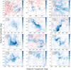 |
Fig. A.1 Distribution of selected sightlines (red crosses) for each cloud, overlaid on the 12CO ( J = 1−0) integrated intensity map from Dame et al. (2001). The cloud name, distance, and number of selected sightlines are labeled in each panel. |
Fitting results of PLM with np = 1–4 for each target cloud.
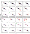 |
Fig. B.1 Fitting results of the piecewise linear model (PLM) with np = 1−4 for each target cloud. The fit models are shown as red lines with shaded confidence intervals, overlaid on the individual measurements. The median trend of log10(W8621/AV) as a function of log10(AV) is shown by the blue squares. The locations of the knots (k) for each PLM are indicated by dashed orange lines. The model selected as optimal for each cloud is marked with a green check mark. The cloud name, distance, and number of sightlines used in the fit are also marked for each cloud. |
All Tables
All Figures
|
Fig. 1 Location of target cloud regions (colored rectangles with names marked below), overplotted on 12CO (J = 1-0) intensity map from Dame et al. (2001). |
| In the text | |
|
Fig. 2 Variation in log10(W8621/AV) as a function of log10(AV) for each target cloud. The corresponding AV scale is shown at the top of each panel. The points are color-coded by their number density, estimated via a Gaussian KDE. The blue squares represent the median log10(W8621/AV) in bins of log10(AV) (from −0.8 to 0.6 with a step of 0.1). The solid red line and shaded region show the selected PLM and its 99.7% credible interval, respectively. The vertical dashed orange lines indicate the knot locations (see Sect. 3.1). The full PLM fitting results with np = 1−4 for each cloud can be found in Fig. B.1. For Cepheus South, the points marked with black crosses were clipped as outliers and excluded from the fit (see Sect. 4 for details). Each panel is labeled with the cloud name, distance, and the number of sightlines. |
| In the text | |
|
Fig. 3 Comparison of the slopes and knots of the selected PLM between target clouds. The slopes are arranged with increasing log10(AV) and are marked with different colors. |
| In the text | |
|
Fig. 4 Linear fit to the relation between log10(W8621/EB-V) and EB-V for sightlines in the Taurus cloud with EB-V < 0.2 mag. The data points included in the fit are shown as red squares. The best-fit line is shown in red, and the resulting slope (αT) and the Pearson correlation coefficient (rp) are indicated. |
| In the text | |
|
Fig. 5 Theoretical relation between the ionization potential (EIP) of a DIB carrier and the expected observational slope (αT) from the PIE model of S97. The relation is plotted for three different RV = 3.1,4.0, and 5.5. The vertical orange line and shaded region represent our measured value of αT for DIB λ8621 (from Fig. 4) and its 1σ uncertainty, respectively. The intersection of our measurement with the RV = 3.1 curve implies EIP ≈ 12 eV. |
| In the text | |
|
Fig. 6 Upper panel : normalized dust density profiles toward the sightline of (l, b) = (216.9°,−18.6°) in Orion A (432 pc), with a background star at 936 pc. The profiles are derived from the dust maps of Lallement et al. (2022, L22, blue) and Edenhofer et al. (2024, E24, red). The dashed vertical lines indicate the detected dust components. Lower panel: the heatmap of the number of the detected dust components (Npeaks) for the 67 sightlines in Orion A derived with the dust maps of L22 and E24. The color scale and numbers represent that both maps detect a specific number of Npeaks (e.g., 6 sightlines have Npeaks = 4 in L22 and E24). |
| In the text | |
|
Fig. 7 Variation in log10(W8621/AV) as a function of log10(AV) for each target cloud, color-coded by Npeaks of each sightline derived from the E24 map. |
| In the text | |
|
Fig. A.1 Distribution of selected sightlines (red crosses) for each cloud, overlaid on the 12CO ( J = 1−0) integrated intensity map from Dame et al. (2001). The cloud name, distance, and number of selected sightlines are labeled in each panel. |
| In the text | |
|
Fig. B.1 Fitting results of the piecewise linear model (PLM) with np = 1−4 for each target cloud. The fit models are shown as red lines with shaded confidence intervals, overlaid on the individual measurements. The median trend of log10(W8621/AV) as a function of log10(AV) is shown by the blue squares. The locations of the knots (k) for each PLM are indicated by dashed orange lines. The model selected as optimal for each cloud is marked with a green check mark. The cloud name, distance, and number of sightlines used in the fit are also marked for each cloud. |
| In the text | |
Current usage metrics show cumulative count of Article Views (full-text article views including HTML views, PDF and ePub downloads, according to the available data) and Abstracts Views on Vision4Press platform.
Data correspond to usage on the plateform after 2015. The current usage metrics is available 48-96 hours after online publication and is updated daily on week days.
Initial download of the metrics may take a while.