| Issue |
A&A
Volume 708, April 2026
|
|
|---|---|---|
| Article Number | A131 | |
| Number of page(s) | 13 | |
| Section | Planets, planetary systems, and small bodies | |
| DOI | https://doi.org/10.1051/0004-6361/202557911 | |
| Published online | 08 April 2026 | |
Mean temperature of a spherical body on an elliptic orbit
1
Department of Mathematics, University of Pisa,
Largo Bruno Pontecorvo 5,
56127
Pisa,
Italy
2
Institute of Astronomy, Charles University,
V Holešovičkách 2,
180 00
Prague 8,
Czech Republic
★ Corresponding authors: This email address is being protected from spambots. You need JavaScript enabled to view it.
; This email address is being protected from spambots. You need JavaScript enabled to view it.
; This email address is being protected from spambots. You need JavaScript enabled to view it.
Received:
30
October
2025
Accepted:
23
January
2026
Abstract
Context. The accurate determination of thermal accelerations acting on small bodies orbiting the Sun requires knowing the surface temperature at any moment. In analytical methods, the computation of the temperature is often simplified by assuming that it varies slightly about a constant value. This ansatz allows us to conveniently linearize the problem.
Aims. However, the mean temperature is constant only in the case of a circular orbit. Our aim is to define a time-dependent temperature that would closely represent the mean temperature of a spherical body revolving around the Sun on an eccentric orbit.
Methods. We adopted a model of the mean temperature with a radial profile inside the body and expressed it by superposing the eigenfunctions of the heat diffusion problem. These were represented with Fourier series in a time domain and spherical Bessel functions in the space domain. The coefficients that weight the contribution of each term were determined from the boundary conditions. Special care was taken to properly account for the non-linearity of the surface energy balance.
Results. We developed a robust algorithm to obtain the coefficients of the mean temperature series and tested the results for various choices in their truncation. Degree eight appears to be adequate for orbits up to eccentricity ≃0.4. The thermal parameter may have an arbitrary value, including limits of both zero and infinite thermal inertia of the surface. The size of the body may also be arbitrary. We provide simplified results for the small- and large-body limits, with the penetration depth of the seasonal thermal wave being the length scale.
Conclusions. Our formulation of the mean temperature offers the possibility to develop an analytical description of seasonal and diurnal variants of thermal accelerations, including their coupling for an eccentric orbit. Previous models are thus generalized.
Key words: celestial mechanics / minor planets, asteroids: general
© The Authors 2026
 Open Access article, published by EDP Sciences, under the terms of the Creative Commons Attribution License (https://creativecommons.org/licenses/by/4.0), which permits unrestricted use, distribution, and reproduction in any medium, provided the original work is properly cited.
This article is published in open access under the Subscribe to Open model. This email address is being protected from spambots. You need JavaScript enabled to view it. to support open access publication.
1 Introduction
Determination of the temperature averaged over the surface of bodies orbiting the Sun (thereafter, the mean temperature) is a useful information for studies of numerous physical processes in planetary science. We consider an analysis of the non-gravitational accelerations due to absorption and subsequent thermal reemission of sunlight, termed the Yarkovsky effect (review of its multiple applications in dynamics of small bodies in the Solar system may be found in Bottke et al. 2006; Vokrouhlický et al. 2015). The high-accuracy models of the Yarkovsky effect that can account for shape irregularities at all length scales, variable thermal parameters, or complex rotation state, require a fully numerical setup. This approach is needed, but generally requires a significant computational time and often does not provide information about the sensitivity of the results on multiple physical parameters. In contrast, analytical models of the Yarkovsky effect resort to approximations and thus only provide low-accuracy results, but are generally fast and offer the possibility to directly understand the dependence on the physical parameters. The aim of this paper is to generalize previous analytical models of the Yarkovsky effect.
The problem of the heat conduction and reemission is at the core of modelling the Yarkovsky effect. This requires solving the heat diffusion equation in the body with appropriate boundary conditions. In spite of approximating the shape by simple geometries (e.g., ellipsoidal or even spherical), the boundary condition that expresses the energy balance at the surface still presents a difficult problem because the thermally reemitted energy depends on the fourth power of the surface temperature and is therefore strongly non-linear. The analytical methods used to determine the Yarkovsky effect generally resort to a linearization of the thermal reemission term at the surface by assuming that the temperature can be split to a suitably chosen constant value and a small variation1 (e.g., Afonso et al. 1995; Rubincam 1998; Farinella et al. 1998; Vokrouhlický 1998a,b; Mysen 2008). While providing reasonable results, the assumption of a constant mean temperature is fairly restrictive and adequate to the case of bodies on circular or low-eccentricity orbits.
The aim of this work is to provide a fully analytical formulation of the mean temperature that is suitable for either a linear or a non-linear analysis of the Yarkovsky effect that perturbs the motion of a body on an eccentric heliocentric orbit. While the principal part of the thermal effects modelling is intended for a forthcoming publication, the mean temperature should ideally contain information about part of the seasonal component (including the delay between absorption and reemission due to finite thermal inertia). In order to achieve this goal, we defined the mean temperature Tav as an exact solution of the heat diffusion problem and neglected diurnal effects. This allowed us to assume that Tav only has a radial profile inside the body and that the solar radiation flux is simply represented by its average value over the whole surface at a given heliocentric distance (Sect. 2). This setup resembles earlier thermal models of comets (see, e.g., Kuehrt 1984), with a few exceptions: no activity is assumed in our case, or the physical parameters are considered constant. On the other hand, cometary models are often restricted to modelling subsurface thermal processes assuming an isothermal core (the large-body limit in our terminology), while we treated all regimes of the ratio of the body size and penetration depth of the thermal effects. The cometary models mostly used a numerical approach, while we provide an analytical solution here. The method of its construction is discussed Sect. 3. Finally, we provide in Sect. 4 examples of our results and test the limits of their applicability. Because of the practical necessity of truncating the infinite series representing our solution, we are mostly concerned with the maximum value of the orbital eccentricity for which it can be used.
2 Formulation of the problem
We considered a spherical body with a radius R orbiting the Sun on an elliptical orbit with an eccentricity e. We assumed uniform rotation with the frequency ω about the spin axis s fixed in the inertial space. Adopting a body frame ℬ with the z-axis along the spin vector s, we wished to determine the temperature T(t; r) at an arbitrary time t and location r within the body. To do this, we needed to solve the heat conduction equation,
![Mathematical equation: $\[\rho C \frac{\partial T}{\partial t}=K \nabla^2 T.\]$](/articles/aa/full_html/2026/04/aa57911-25/aa57911-25-eq1.png) (1)
(1)
For the sake of simplicity, we assumed all physical parameters, such as the bulk density ρ, the specific heat C, and the thermal conductivity K, to be constant. Given the assumed spherical shape of the body, we adopted spherical coordinates (r, θ, φ) to describe r in the body frame ℬ.
The linear dependence of Eq. (1) on T allowed us an analytical solution in terms of its development in a system of properly chosen eigenfunctions (Sect. 3). The free coefficients of this decomposition need to be determined by the boundary conditions. We assumed periodicity of the solution with a period Prev of the revolution about the Sun for the time domain. Following Vokrouhlický (1999), we assumed that the rotation period Prot of the body was commensurable with Prev, such that Prev/Prot = m ≫ 1. Moreover, as shown in Farinella & Vokrouhlický (1996), it is possible to extend this result to the case of real m when the timescales of the variation in the spin-axis orientation are longer than the rotation and revolution periods. We assumed a constant spin rate and principal-axis rotation for simplicity. The boundary conditions of the space domain included (i) the regularity of T in the centre of the body r = 0, and (ii) the energy conservation at its surface,
![Mathematical equation: $\[\epsilon \sigma T^4+\left.K \frac{\partial T}{\partial r}\right|_{r=R}=\alpha \mathcal{E},\]$](/articles/aa/full_html/2026/04/aa57911-25/aa57911-25-eq2.png) (2)
(2)
which expresses balance between the energy radiated by an arbitrary surface element using a grey-body approximation with emissivity ϵ (σ being the Stefan-Boltzmann constant), the energy conducted to the subsurface layers, and the solar radiation energy absorbed by the surface element. The latter was decomposed into the absorption coefficient α and the incident solar radiation flux projected onto the normal vector of the surface element.
The non-linear dependence of the boundary condition (2) on T represents a major obstacle to the analytic solution of the problem. This issue is traditionally overcome by assuming that T is close enough to a certain average value Tav, such that T(t; r = Tav + ΔT(t; r) and ΔT/Tav ≪ 1 for arbitrary t and r in the solution domain. Taking the approximation ![Mathematical equation: $\[T^{4} \approx T_{\mathrm{av}}^{4}+4 T_{\mathrm{av}}^{3} ~\Delta T\]$](/articles/aa/full_html/2026/04/aa57911-25/aa57911-25-eq3.png) implies linearity of the boundary condition (2) in ΔT, allowing us to handle the problem in analytical terms. The choice of Tav is an important part of the procedure. In this respect, most of the previous analyses adopted the simplest assumption of a constant value Tav. In our context, this is well justified for a body revolving about the Sun on a circular orbit, or on an orbit with a very low eccentricity e. However, when e becomes significant, it is difficult to choose a constant Tav value globally, such that the linearization of the T4 term in the boundary conditions (2) still holds.
implies linearity of the boundary condition (2) in ΔT, allowing us to handle the problem in analytical terms. The choice of Tav is an important part of the procedure. In this respect, most of the previous analyses adopted the simplest assumption of a constant value Tav. In our context, this is well justified for a body revolving about the Sun on a circular orbit, or on an orbit with a very low eccentricity e. However, when e becomes significant, it is difficult to choose a constant Tav value globally, such that the linearization of the T4 term in the boundary conditions (2) still holds.
To solve this problem, we propose to keep the linearization scheme, but we dropped the assumption of a constant Tav value. Instead, we considered Tav depending on time t and radial distance r from the body centre. This brings certain algebraic difficulty in expressing the solution analytically to already the average temperature part, but it leaves the principles how to solve ΔT as before. We postpone the solution of ΔT to a future work and focus here on the novel aspect of the approach, namely the determination of Tav.
Tav as a function of t and r must satisfy the following set of equations:
![Mathematical equation: $\[\rho C \frac{\partial T_{\mathrm{av}}}{\partial t}=\frac{K}{r^2} \frac{\partial}{\partial r}\left(r^2 \frac{\partial}{\partial r}\right) T_{\mathrm{av}},\]$](/articles/aa/full_html/2026/04/aa57911-25/aa57911-25-eq4.png) (3)
(3)
![Mathematical equation: $\[\epsilon \sigma T_{\mathrm{av}}^4+\left.K \frac{\partial T_{\mathrm{av}}}{\partial r}\right|_{r=R}=\alpha \overline{\mathcal{E}},\]$](/articles/aa/full_html/2026/04/aa57911-25/aa57911-25-eq5.png) (4)
(4)
where ![Mathematical equation: $\[\overline{\mathcal{E}}=\overline{\mathcal{E}}(t)\]$](/articles/aa/full_html/2026/04/aa57911-25/aa57911-25-eq6.png) is a characteristic mean insolation of the body at time t. The previous analyses of the insolation of a sphere (e.g., Vokrouhlický 1998a; Čapek & Vokrouhlický 2010) have shown that
is a characteristic mean insolation of the body at time t. The previous analyses of the insolation of a sphere (e.g., Vokrouhlický 1998a; Čapek & Vokrouhlický 2010) have shown that ![Mathematical equation: $\[\overline{\mathcal{E}}=F(t) / 4\]$](/articles/aa/full_html/2026/04/aa57911-25/aa57911-25-eq7.png) , where F(t) is the solar radiation flux at time t. The time dependence in F is simply due to the changing heliocentric distance d along the elliptic orbit and F ∝ 1/d2.
, where F(t) is the solar radiation flux at time t. The time dependence in F is simply due to the changing heliocentric distance d along the elliptic orbit and F ∝ 1/d2.
Before we proceed to the analytical solution of Tav, we simplified Eqs. (3) and (4) by appropriately scaling all variables. This step allowed us to highlight the single fundamental parameter of the problem (aside from the orbital eccentricity e). As in Vokrouhlický (1998a, 1999), we adopted the following replacement rules:
t → ζ, with a complex variable ζ = eιℓ and ℓ the mean anomaly of the elliptic motion about the Sun and
![Mathematical equation: $\[\iota=\sqrt{-1}\]$](/articles/aa/full_html/2026/04/aa57911-25/aa57911-25-eq8.png) ;
;r → r′, defined by r′ = r/hs, where
![Mathematical equation: $\[h_{\mathrm{s}}=\sqrt{K / \rho C n}\]$](/articles/aa/full_html/2026/04/aa57911-25/aa57911-25-eq9.png) is the depth of the seasonal thermal wave and n the mean motion of the body about the Sun;
is the depth of the seasonal thermal wave and n the mean motion of the body about the Sun;F → F′, defined by F′ = F/Fa, where Fa is the solar radiation flux at a distance d equal to the semi-major axis a of the heliocentric orbit;
![Mathematical equation: $\[T_{\mathrm{av}} \rightarrow T_{\mathrm{av}}^{\prime}=T_{\mathrm{av}} / T_{a}\]$](/articles/aa/full_html/2026/04/aa57911-25/aa57911-25-eq10.png) , with the reference temperature Ta defined by
, with the reference temperature Ta defined by ![Mathematical equation: $\[\epsilon \sigma T_{a}^{4}=\alpha F_{a}\]$](/articles/aa/full_html/2026/04/aa57911-25/aa57911-25-eq11.png) .
.
Plugging these new variables into Eqs. (3) and (4), we obtained (R′ = R/hs),
![Mathematical equation: $\[\imath \frac{\partial T_{\mathrm{av}}^{\prime}}{\partial \zeta}=\frac{1}{r^{\prime 2}} \frac{\partial}{\partial r^{\prime}}\left(r^{\prime 2} \frac{\partial}{\partial r^{\prime}}\right) T_{\mathrm{av}}^{\prime},\]$](/articles/aa/full_html/2026/04/aa57911-25/aa57911-25-eq12.png) (5)
(5)
![Mathematical equation: $\[T_{\mathrm{av}}^{\prime 4}+\left.\Theta \frac{\partial T_{\mathrm{av}}^{\prime}}{\partial r^{\prime}}\right|_{r^{\prime}=R^{\prime}}=\overline{\mathcal{E}}^{\prime},\]$](/articles/aa/full_html/2026/04/aa57911-25/aa57911-25-eq13.png) (6)
(6)
indicating that the problem depends on two fundamental parameters. The first, ![Mathematical equation: $\[\Theta=\sqrt{K \rho C} \sqrt{n} /\left(\epsilon \sigma T_{a}^{3}\right)\]$](/articles/aa/full_html/2026/04/aa57911-25/aa57911-25-eq14.png) is explicitly displayed in (6) and is usually called the thermal parameter. The second, the eccentricity e of the heliocentric orbit, is implicitly present in the expression of the scaled insolation term on the right side of (6), which reads
is explicitly displayed in (6) and is usually called the thermal parameter. The second, the eccentricity e of the heliocentric orbit, is implicitly present in the expression of the scaled insolation term on the right side of (6), which reads
![Mathematical equation: $\[\overline{\mathcal{E}}^{\prime}=\frac{1}{4}\left(\frac{a}{d}\right)^2.\]$](/articles/aa/full_html/2026/04/aa57911-25/aa57911-25-eq15.png) (7)
(7)
In order to express it using ζ and e, we used an elliptic expansion,
![Mathematical equation: $\[\overline{\mathcal{E}}^{\prime}=\frac{1}{4} \sum_{n \in Z} a_n(e) \zeta^n,\]$](/articles/aa/full_html/2026/04/aa57911-25/aa57911-25-eq16.png) (8)
(8)
where an are the Hansen coefficients ![Mathematical equation: $\[a_{n}=X_{n}^{-2,0}(e)\]$](/articles/aa/full_html/2026/04/aa57911-25/aa57911-25-eq17.png) , obeying an important property an ≃ 𝒪(e|n|). The zero-order coefficient is
, obeying an important property an ≃ 𝒪(e|n|). The zero-order coefficient is ![Mathematical equation: $\[a_{0}=1 / \sqrt{1-e^{2}}\]$](/articles/aa/full_html/2026/04/aa57911-25/aa57911-25-eq18.png) . Because of the faster convergence, we chose to expand the an coefficients in terms of
. Because of the faster convergence, we chose to expand the an coefficients in terms of ![Mathematical equation: $\[\beta=\frac{e}{1+\sqrt{1-e^{2}}}\]$](/articles/aa/full_html/2026/04/aa57911-25/aa57911-25-eq19.png) instead of e. The leading coefficient thus reads a0 = (1 + β2)/(1 − β2), while in general, we have
instead of e. The leading coefficient thus reads a0 = (1 + β2)/(1 − β2), while in general, we have
![Mathematical equation: $\[a_n=\beta^{|n|} \sum_{\ell=0}^{\infty} a_{n,|n|+2 \ell} \beta^{2 \ell},\]$](/articles/aa/full_html/2026/04/aa57911-25/aa57911-25-eq20.png) (9)
(9)
with a certain set of numerical constants ai,j (e.g., Tisserand 1894; Breiter et al. 2004). The lowest-degree coefficients an (n ≤ 8) read
![Mathematical equation: $\[\begin{aligned}& a_0=1+2 \beta^2+2 \beta^4+2 \beta^6+2 \beta^8, \\& a_1=2 \beta+\beta^3+\frac{23}{6} \beta^5+\frac{73}{72} \beta^7, \\& a_2=5 \beta^2-\frac{22}{3} \beta^4+\frac{76}{3} \beta^6-\frac{2254}{45} \beta^8, \\& a_3=13 \beta^3-\frac{181}{4} \beta^5+\frac{1267}{8} \beta^8, \\& a_4=\frac{103}{3} \beta^4-\frac{2834}{15} \beta^6+\frac{36074}{45} \beta^8, \\& a_5=\frac{1097}{12} \beta^5-\frac{49531}{72} \beta^7, \\& a_6=\frac{1223}{5} \beta^6-\frac{81722}{35} \beta^8, \\& a_7=\frac{47273}{72} \beta^7, \\& a_8=\frac{556403}{310} \beta^8,\end{aligned}\]$](/articles/aa/full_html/2026/04/aa57911-25/aa57911-25-eq21.png)
where terms to the order eight in β were included.
We point out that the above expansion are convergent only when e < eL, where eL ~ 0.66 is the Laplace limit (Da Silva Fernandes 1995). The iterative procedure described in the following section relies on the convergence of the Hansen coefficients expansion, and we therefore consider an object with eccentricity e < eL in the following.
3 The average temperature solution
In this section, we provide the algorithm for determining ![Mathematical equation: $\[T_{\mathrm{av}}^{\prime}\]$](/articles/aa/full_html/2026/04/aa57911-25/aa57911-25-eq22.png) . The linearity of the heat conduction equation (5) makes the solution still simple, but the eigenfunctions of the differential operator on the right side should be observed. These are the spherical Bessel functions of the first kind and degree zero j0 (the Bessel functions of the second kind are excluded by regularity of the solution at r′ = 0), while the eigenfunctions of the time operator on the right side of (5) are simply powers ζn (or Fourier series in ℓ if set in real notation). The general solution thus reads
. The linearity of the heat conduction equation (5) makes the solution still simple, but the eigenfunctions of the differential operator on the right side should be observed. These are the spherical Bessel functions of the first kind and degree zero j0 (the Bessel functions of the second kind are excluded by regularity of the solution at r′ = 0), while the eigenfunctions of the time operator on the right side of (5) are simply powers ζn (or Fourier series in ℓ if set in real notation). The general solution thus reads
![Mathematical equation: $\[T_{\mathrm{av}}^{\prime}\left(\zeta, r^{\prime}\right)=\sum_{n \in \mathbb{Z}} c_n \zeta^n j_0\left(z_n\right),\]$](/articles/aa/full_html/2026/04/aa57911-25/aa57911-25-eq23.png) (10)
(10)
where ![Mathematical equation: $\[z_{n}=\sqrt{-i n} r^{\prime}\]$](/articles/aa/full_html/2026/04/aa57911-25/aa57911-25-eq24.png) . We note that
. We note that ![Mathematical equation: $\[T_{\mathrm{av}}^{\prime}\]$](/articles/aa/full_html/2026/04/aa57911-25/aa57911-25-eq25.png) must be real, which implies that cn are complex coefficients and c−n must be complex-conjugated to cn. Their value has to be determined from the boundary condition (6), with the algebraic challenge to deal with non-linearity of the
must be real, which implies that cn are complex coefficients and c−n must be complex-conjugated to cn. Their value has to be determined from the boundary condition (6), with the algebraic challenge to deal with non-linearity of the ![Mathematical equation: $\[T_{\mathrm{av}}^{\prime 4}\]$](/articles/aa/full_html/2026/04/aa57911-25/aa57911-25-eq26.png) term. In particular, plugging in the solution (10) directly to (6), and separating the n = 0 terms, we have
term. In particular, plugging in the solution (10) directly to (6), and separating the n = 0 terms, we have
![Mathematical equation: $\[\begin{aligned}& \overbrace{\left[c_0+\sum_{n \neq 0} c_n \zeta^n j_0\left(Z_n\right)\right]^4}^{T_{\mathrm{av}}^{\prime 4}}+\overbrace{\Theta \frac{\partial}{\partial r^{\prime}}\left[\sum_{n \neq 0} c_n \zeta^n j_0\left(z_n\right)\right]_{z_n=\sqrt{-i n} R^{\prime}}}^{\left.\Theta \frac{\partial}{\partial r^{\prime}} T_{\mathrm{av}}^{\prime}\right|_{r=R^{\prime}}} \\& \quad=\frac{a_0}{4}+\frac{1}{4} \sum_{n \neq 0} a_n \zeta^n.\end{aligned}\]$](/articles/aa/full_html/2026/04/aa57911-25/aa57911-25-eq27.png) (11)
(11)
Further algebra simplifies with replacing cn by Cn = cn j0 (Zn), where ![Mathematical equation: $\[z_{n}=\sqrt{-i n} R^{\prime}\]$](/articles/aa/full_html/2026/04/aa57911-25/aa57911-25-eq28.png) , and by introducing
, and by introducing
![Mathematical equation: $\[\psi_n=\left.\frac{z}{j_0(z)} \frac{d j_0}{d z}\right|_{z=Z_n}.\]$](/articles/aa/full_html/2026/04/aa57911-25/aa57911-25-eq29.png) (12)
(12)
The boundary condition (11) then reads
![Mathematical equation: $\[\left[C_0+\sum_{n \neq 0} C_n \zeta^n\right]^4+\frac{\Theta}{R^{\prime}} \sum_{n \neq 0} C_n \psi_n \zeta^n=\frac{a_0}{4}+\frac{1}{4} \sum_{n \neq 0} a_n \zeta^n.\]$](/articles/aa/full_html/2026/04/aa57911-25/aa57911-25-eq30.png) (13)
(13)
The remaining algebra, at higher orders performed with the aid of computer software, stems from (i) comparing terms of the same power in ζ on either side of Eq. (13), and (ii) at the same time developing Cn in power series of β, namely2
![Mathematical equation: $\[C_n=\beta^{|n|} \sum_{\ell=0}^{\infty} C_{n,|n|+2 \ell} \beta^{2 \ell}\]$](/articles/aa/full_html/2026/04/aa57911-25/aa57911-25-eq31.png) (14)
(14)
similar to the series expansion of an in (9). Again, comparison of terms of the same power in β yields a general scheme to determine the numerical coefficients Ci,j. We first illustrate the procedure in Sect. 3.1 by pushing the algorithm to the lowest order in both ζ and β, and we then present the general algorithm in Sect. 3.2.
3.1 First-degree approximation
We describe details of the procedure for computing the average temperature coefficients in the case of a first-degree approximation, namely, approximating
![Mathematical equation: $\[T_{\mathrm{av}}^{\prime}=C_0+C_1 \zeta+C_{-1} \zeta^{-1}.\]$](/articles/aa/full_html/2026/04/aa57911-25/aa57911-25-eq32.png) (15)
(15)
Expanding the fourth-power in the boundary condition, we obtain
![Mathematical equation: $\[\begin{aligned}T_{\mathrm{av}}^{\prime 4}= & C_0^4+12 C_0^2 C_1 C_{-1}+6\left(C_1 C_{-1}\right)^2 \\& +4 C_0\left(C_0^2+3 C_1 C_{-1}\right)\left(C_1 \zeta+C_{-1} \zeta^{-1}\right)+\ldots,\end{aligned}\]$](/articles/aa/full_html/2026/04/aa57911-25/aa57911-25-eq33.png) (16)
(16)
and the boundary condition (13) reads
![Mathematical equation: $\[\begin{aligned}C_0^4 & +6 C_1 C_{-1}\left[2 C_0^2+C_1 C_{-1}\right]+4 C_0\left(C_0^2+3 C_1 C_{-1}\right)\left(C_1 \zeta+C_{-1} \zeta^{-1}\right) \\& +\frac{\Theta}{R^{\prime}}\left(C_1 \psi_1 \zeta+C_{-1} \psi_{-1} \zeta^{-1}\right)+\ldots=\frac{1}{4} \frac{1-\beta^2}{1+\beta^2}+\frac{1}{4}\left(a_1 \zeta+a_{-1} \zeta^{-1}\right)+\ldots.\end{aligned}\]$](/articles/aa/full_html/2026/04/aa57911-25/aa57911-25-eq34.png) (17)
(17)
Recalling that an are power series of β such that an ~ β|n|, we compare terms of the same powers in (ζ, β) on either side of Eq. (17). A brief algebra yields to the order β3
![Mathematical equation: $\[\begin{aligned}& C_{00}^4+4 C_{00}^3 C_{02} \beta^2+12 C_{00}^2 C_{11}^2 C_{-11}^2 \beta^2+4 C_{00}^3 C_{11} \beta \zeta+\frac{\Theta}{R^{\prime}} C_{11} \psi_1 \zeta \\& +C. C.=\frac{1}{4}+\frac{1}{2} \beta^2+\frac{1}{2} \beta \zeta+C. C.,\end{aligned}\]$](/articles/aa/full_html/2026/04/aa57911-25/aa57911-25-eq35.png) (18)
(18)
where C.C. stands for the complex conjugate terms. Observing equal powers in β and ζ on either side of (18), we obtain
![Mathematical equation: $\[C_{00}=\frac{1}{\sqrt{2}}\]$](/articles/aa/full_html/2026/04/aa57911-25/aa57911-25-eq36.png) (19)
(19)
at the zero order (completing C0 to 𝒪(β2)), and
![Mathematical equation: $\[C_{11}=\frac{1}{2 \sqrt{2}} \frac{1}{1+\frac{\Theta}{\sqrt{2} R^{\prime}} \psi_1}\]$](/articles/aa/full_html/2026/04/aa57911-25/aa57911-25-eq37.png) (20)
(20)
at the first order (completing C1 to 𝒪(β3)). Clearly, the C−11 coefficient is obtained by taking the complex conjugate of C11.
Remark. Although in principle we could fix the degree of the approximation and increase the order, the formulas behave better when we keep the order of the approximation lower than the maximum degree, as shown in the following.
3.2 Algorithm
In this section, we describe an iterative algorithm for computing the coefficients Cnj, which are functions of the thermal parameter Θ and of the normalized radius R′. The following properties imply that the algorithm is well-defined.
Proposition.
Linearity, that is, the coefficient Cnj, can be computed through a first-order linear relation that only involves terms of lower degree and order.
Cnj only depends on the terms Cmk for which the following relations hold:
![Mathematical equation: $\[0 \leq k+m \leq j+n,\]$](/articles/aa/full_html/2026/04/aa57911-25/aa57911-25-eq38.png) (21)
(21)
![Mathematical equation: $\[0 \leq k-m \leq j-n.\]$](/articles/aa/full_html/2026/04/aa57911-25/aa57911-25-eq39.png) (22)
(22)
Proof.
-
We focus on a generic coefficient Cnj. First of all, we note that by definition, we have that
![Mathematical equation: $\[j \geq|n|,\]$](/articles/aa/full_html/2026/04/aa57911-25/aa57911-25-eq40.png) (23)
(23)so that j + n ≥ 0 and j − n ≥ 0. Moreover, we have that j ≡ n (mod 2). The lowest degree and order at which the coefficient Cnj appears in the boundary condition (18) is degree n and order j. We focus on the left side of the boundary condition equation. Because of the definition of
![Mathematical equation: $\[T_{\mathrm{av}}^{\prime}\]$](/articles/aa/full_html/2026/04/aa57911-25/aa57911-25-eq41.png) and of Cnj, the above statement is straightforward for the second sum. On the other hand, we consider the form of a generic term in the multinomial expansion of the fourth-power term. This term is proportional to
and of Cnj, the above statement is straightforward for the second sum. On the other hand, we consider the form of a generic term in the multinomial expansion of the fourth-power term. This term is proportional to
![Mathematical equation: $\[C_{i_1}^{k_1} C_{i_2}^{k_2} C_{i_3}^{k_3} C_{i_4}^{k_4} \zeta^{k_1 i_1+k_2 i_2+k_3 i_3+k_4 i_4},\]$](/articles/aa/full_html/2026/04/aa57911-25/aa57911-25-eq42.png) (24)
(24)where the positive integers k1, k2, k3, and k4 verify
![Mathematical equation: $\[k_1+k_2+k_3+k_4=4.\]$](/articles/aa/full_html/2026/04/aa57911-25/aa57911-25-eq43.png) (25)
(25)Therefore, we can focus on terms of the form
![Mathematical equation: $\[\begin{array}{lcc}C_p^4 \zeta^{4 p} \qquad C_p^3 C_q \zeta^{3 p+q} \qquad C_p^2 C_q^2 \zeta^{2(p+q)} \\C_p^2 C_q C_r \zeta^{2 p+q+r}\qquad C_p C_q C_r C_s \zeta^{p+q+r+s}.\end{array}\]$](/articles/aa/full_html/2026/04/aa57911-25/aa57911-25-eq44.png) (26)
(26)These relations can be readapted in terms of the expansion in series of β,
![Mathematical equation: $\[\begin{aligned}& C_{p g}^4 \zeta^{4 p} \beta^{4 g} \quad C_{p g}^3 C_{q h} \zeta^{3 p+q} \beta^{3 g+h} \quad C_{p g}^2 C_{q, h}^2 \zeta^{2(p+q)} \beta^{2(g+h)} \\& C_{p g}^2 C_{q h} C_{r i} \zeta^{2 p+q+r} \beta^{2 g+h+i} \quad C_{p g} C_{q h} C_{r i} C_{s l} \zeta^{p+q+r+s} \beta^{g+h+i+l}.\end{aligned}\]$](/articles/aa/full_html/2026/04/aa57911-25/aa57911-25-eq45.png) (27)
(27)Therefore, the lowest degree and order term in which Cnj appears must have the form
![Mathematical equation: $\[C_{00}^3 C_{n j} \zeta^n \beta^j.\]$](/articles/aa/full_html/2026/04/aa57911-25/aa57911-25-eq46.png) (28)
(28)Therefore, because of the previous considerations, it is possible to obtain Cnj as the solution of an equation of the form
![Mathematical equation: $\[F C_{n j}=G,\]$](/articles/aa/full_html/2026/04/aa57911-25/aa57911-25-eq47.png) (29)
(29)where F and G are functions of the coefficients Cmk with m < n and k < j.
-
We present a maximal set of coefficient that appear in the definition of Cnj. To do this, we focus on the terms of degree n and order j in the boundary condition. Selecting these terms is trivial in the case of the right side of the equation, while it is more challenging in the case of the left side because of the fourth-power term. By focusing on the form of the generic terms appearing in the expansion (which we presented above), we develop formulas that identify the required coefficients. Without loss of generality, we focus on a term of the form
![Mathematical equation: $\[C_{00}^2 C_{m k} C_{n-m, j-k},\]$](/articles/aa/full_html/2026/04/aa57911-25/aa57911-25-eq48.png) (30)
(30)which is a term of degree n and order j. The relation involving the indices of the required coefficients is obtained by remarking that because of condition (23), we have that it must hold that k ≥ |m| and
![Mathematical equation: $\[j-k \geq|n-m|.\]$](/articles/aa/full_html/2026/04/aa57911-25/aa57911-25-eq49.png) (31)
(31)Therefore, we have that
![Mathematical equation: $\[k \pm m \geq 0\]$](/articles/aa/full_html/2026/04/aa57911-25/aa57911-25-eq50.png) (32)
(32)and that
![Mathematical equation: $\[j-k \pm|n-m| \geq 0.\]$](/articles/aa/full_html/2026/04/aa57911-25/aa57911-25-eq51.png) (33)
(33)These two relations imply the thesis. Focusing on terms Cmk with m, k ≠ 0 that appear with an exponent higher than 1 would naturally yield only a subset of the coefficients described by the relation above.
3.2.1 Description of the algorithm
We started by selecting the maximum degree nmax at which we truncated the series for the normalized average temperature, namely
![Mathematical equation: $\[T_{\mathrm{av}}^{\prime} \simeq \sum_{n=-n_{\max }}^{n_{\max }} C_n \zeta^n.\]$](/articles/aa/full_html/2026/04/aa57911-25/aa57911-25-eq52.png) (34)
(34)
Because of the properties of the second part of the above proposition, an efficient method of computing the coefficient is the following.
First, compute all the diagonal coefficients Cnn up to n = nmax and with n ≥ 0. Because of the properties of the Cnj, by taking the complex conjugate of the diagonal coefficients, we obtain C−n,n n = 1, . . ., nmax.
Compute the coefficients in the above diagonal as shown by the blue arrows in Fig. 1, i.e. the Cn,n+2 up to n = nmax −2.
Iterate the procedure by focusing on the next diagonal until all the coefficients are computed.
In principle, the procedure described above could be extended to arbitrary degree and order, but it is well defined only within the radius of convergence of the series expansion of the Hansen coefficients, that is, e < eL.
Remark. A key feature of this procedure is that when we wish to increase the fidelity of the model by increasing the degree of the truncation, it is not necessary to recompute all coefficients, but only the new ones, as shown by the shaded areas in Fig. 1.
3.2.2 Example: computation of the coefficient up to degree and order 2
After outlining the general algorithm, we found it useful to illustrate it in the case of pushing the first-order solution from Sect. 3.1 to the second order, determining thus coefficients C02 and C22. To compute the diagonal coefficient C22, we focused on the boundary condition. Given that ![Mathematical equation: $\[C_{00}=1 / \sqrt{2}\]$](/articles/aa/full_html/2026/04/aa57911-25/aa57911-25-eq53.png) and C11 in (20), the terms of degree and order 2 of the boundary condition read
and C11 in (20), the terms of degree and order 2 of the boundary condition read
![Mathematical equation: $\[3 C_{11}^2+\sqrt{2} C_{22}+\frac{\Theta}{R^{\prime}} C_{22}=\frac{5}{4},\]$](/articles/aa/full_html/2026/04/aa57911-25/aa57911-25-eq54.png) (35)
(35)
from which we obtained
![Mathematical equation: $\[C_{22}=\frac{5-12 C_{11}^2}{4 \sqrt{2}} \frac{1}{1+\frac{\Theta}{\sqrt{2} R^{\prime}} \psi_2}.\]$](/articles/aa/full_html/2026/04/aa57911-25/aa57911-25-eq55.png) (36)
(36)
To compute C02, we proceeded similarly, but focused this time on the terms of degree 0 and order 2 of the boundary conditions, which read
![Mathematical equation: $\[\sqrt{2} C_{02}+6 C_{11} C_{-11}=\frac{1}{2}.\]$](/articles/aa/full_html/2026/04/aa57911-25/aa57911-25-eq56.png) (37)
(37)
Solving for C02, we obtained
![Mathematical equation: $\[C_{02}=\frac{1-12 C_{11} C_{-11}}{2 \sqrt{2}}.\]$](/articles/aa/full_html/2026/04/aa57911-25/aa57911-25-eq57.png) (38)
(38)
In the next section, we describe the asymptotic behaviour of the coefficients with respect to the normalized radius R′ in order to simplify formulas similar to Eq. (35).
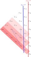 |
Fig. 1 Flow chart for determining coefficients Cnk up to nmax = 4. The algorithm proceeds in the order indicated by the blue arrows. The shaded areas show that when nmax is increased to 5, most of the needed coefficients are already known, and it suffices to only compute three new ones: C15, C35, and C55. |
3.3 Limits of large and small bodies
The surface temperature, determined by coefficients Cn, is a non-trivial function of the scaled size R′, principally due to their dependence on complex factors ψn. However, as a general rule of thumb, there are two regimes with a transition close to R′ ≃ 1. This is when the physical size is comparable to the penetration depth of the seasonal thermal wave3. For lower R′ values, the imaginary part of Cn decreases inversely proportionally to R′, while the real part of Cn converges to particular values independent of Θ. In contrast, for higher R′ values, the real and imaginary parts of Cn both converge to constant values dependent on Θ. The asymptotic values in both limits also depend on the orbital eccentricity. We now describe the two limiting regimes of small (R′ ≪ 1) and large (R′ ≫ 1) bodies with a few more details. To do this, we introduce the following auxiliary functions (n ≥ 0, the case of negative n values is not needed since ψ−n is complex conjugate to ψn):
![Mathematical equation: $\[G_n^{ \pm} \equiv 1-e^{-4 x_n} \pm 2 e^{-2 x_n} ~\sin~ 2 x_n,\]$](/articles/aa/full_html/2026/04/aa57911-25/aa57911-25-eq58.png) (39)
(39)
![Mathematical equation: $\[F_n \equiv 1+e^{-4 x_n}-2 e^{-2 x_n} ~\cos~ 2 x_n,\]$](/articles/aa/full_html/2026/04/aa57911-25/aa57911-25-eq59.png) (40)
(40)
which are related to the real and imaginary parts of ψn as follows:
![Mathematical equation: $\[\psi_n=\frac{x_n\left(G_n^{+}+\imath G_n^{-}\right)}{F_n}-1,\]$](/articles/aa/full_html/2026/04/aa57911-25/aa57911-25-eq60.png) (41)
(41)
with ![Mathematical equation: $\[x_{n}=\sqrt{n / 2} R^{\prime}\]$](/articles/aa/full_html/2026/04/aa57911-25/aa57911-25-eq61.png) . The imaginary part of ψn, namely
. The imaginary part of ψn, namely ![Mathematical equation: $\[x_{n} G_{n}^{-} / F_{n}\]$](/articles/aa/full_html/2026/04/aa57911-25/aa57911-25-eq62.png) , plays the key role in the time offset of the thermal response to orbital forcing represented by elliptic expansion in ζn (see Eq. (13)). In physical terms, it expresses a delay between absorption of sunlight and thermal reemission by the body.
, plays the key role in the time offset of the thermal response to orbital forcing represented by elliptic expansion in ζn (see Eq. (13)). In physical terms, it expresses a delay between absorption of sunlight and thermal reemission by the body.
Small-body limit. In the limit of small bodies, xn → 0, we have
![Mathematical equation: $\[\frac{x_n G_n^{+}}{F_n}-1 \approx-\frac{4}{15} x_n^4+\mathcal{O}\left(x_n^5\right)\]$](/articles/aa/full_html/2026/04/aa57911-25/aa57911-25-eq63.png) (42)
(42)
![Mathematical equation: $\[\frac{x_n G_n^{-}}{F_n} \approx-\frac{2}{3} x_n^2+\mathcal{O}(x_n^3),\]$](/articles/aa/full_html/2026/04/aa57911-25/aa57911-25-eq64.png) (43)
(43)
and thus,
![Mathematical equation: $\[\left.\frac{\psi_n}{x_n}\right|_{x_n \rightarrow 0} \rightarrow 0.\]$](/articles/aa/full_html/2026/04/aa57911-25/aa57911-25-eq65.png) (44)
(44)
This implies that the heat conduction term in the boundary condition (13) is proportional to Θ R′. For a bound value of the thermal inertia, thus Θ, such that Θ R′ → 0, the boundary condition takes a simpler form,
![Mathematical equation: $\[\left(C_0+\sum_{n \neq 0} C_n \zeta^n\right)^4=\frac{1}{4} \frac{1-\beta^2}{1+\beta^2}+\frac{1}{4} \sum_{n \neq 0} a_n \zeta^n,\]$](/articles/aa/full_html/2026/04/aa57911-25/aa57911-25-eq66.png) (45)
(45)
from which the coefficients Cn can again be determined using the above outlined algorithm. Obviously, (45) also implies
![Mathematical equation: $\[T_{\mathrm{av}}^{\prime 4}=\overline{\mathcal{E}}^{\prime},\]$](/articles/aa/full_html/2026/04/aa57911-25/aa57911-25-eq67.png) (46)
(46)
which may be used to verify the result. In physical terms, this limit simply means that very small bodies become isothermal (due to efficient heat conduction across their volume) and the absorbed sunlight energy is instantly re-radiated (since these small bodies cannot store the energy and radiate it with a certain delay). Remarkably, the temperature is just the equilibrium temperature corresponding to the heliocentric distance.
Large-body limit. In the limit of large bodies, xn → ∞, we have G± ≈ F ≈ 1, and therefore,
![Mathematical equation: $\[\frac{\psi_n}{x_n} \approx 1+\imath-\frac{1}{x_n} \xrightarrow[x_n \rightarrow \infty]{ } 1+\imath \text {, }\]$](/articles/aa/full_html/2026/04/aa57911-25/aa57911-25-eq68.png) (47)
(47)
and the boundary condition (13) takes a simplified form,
![Mathematical equation: $\[\left(C_0+\sum_{n \neq 0} C_n \zeta^n\right)^4+\frac{\Theta}{\sqrt{2}} \sum_{n \neq 0} C_n \sqrt{|n|}(1 \pm i) \zeta^n=\frac{1}{4} \frac{1-\beta^2}{1+\beta^2}+\frac{1}{4} \sum_{n \neq 0} a_n \zeta^n,\]$](/articles/aa/full_html/2026/04/aa57911-25/aa57911-25-eq69.png) (48)
(48)
with the positive and negative sign in the bracket of the second term forming positive and negative values of n. Explicit formulas for the Cnj coefficients, computed up to degree and order eight in the large-body limit are presented in Appendix B. Because the penetration depth hs becomes very small compared to the radius R in this limit, all temperature variations become limited to a very narrow skin below the body surface. A description of this situation would benefit from changing the spherical coordinate r, measured from the centre, to a subsurface depth z = R − r (e.g., Vokrouhlický 1998b).
Thermal and dynamical parameters for asteroid Didymos.
4 Surface mean temperature in the large-body limit
We illustrate the mean-temperature algorithm outlined above for a large body with a fixed elliptic orbit. For the sake of the example, we used the orbit and physical parameters of asteroid (65803) Didymos (see Table 1) because of the growing interest in this object as a target of the ESA Hera mission Michel et al. (2022) and Tortora et al. (2025). Our analytical approach is limited, and we therefore only replaced the true Didymos shape by a sphere of an equivalent volume. Assuming thermal conductivity in a plausible range 0.01–0.1 W m−1 K−1 (e.g., Delbó et al. 2015), we estimated that the penetration depth hs of the seasonal thermal wave is between 0.1 and 1 m, which justifies the large-body model for this asteroid well. The data in Table 1 also allowed us to estimate the seasonal thermal parameter Θ ≃ 0.07, which is one of the two principal parameters of the thermal model (Sect. 2). This value is low, but not negligible. Moreover, its analogues associated with higher Fourier terms ![Mathematical equation: $\[\Theta_{n}=\sqrt{n} \Theta\]$](/articles/aa/full_html/2026/04/aa57911-25/aa57911-25-eq70.png) become appreciably larger. The orbital eccentricity e ≃ 0.38 is moderately high and suitable for testing our approach.
become appreciably larger. The orbital eccentricity e ≃ 0.38 is moderately high and suitable for testing our approach.
Figure 2 shows the mean temperature Tav at the surface as a function of the mean anomaly ℓ during a revolution about the Sun for the nominal value of Θ and four selected values of the orbital eccentricity e (including e = 0.38 of Didymos). We tested the effect of series truncation by different values of maximum degree nmax in (34), comparing the results for nmax increasing from 2 to 8. Clearly, restricting to nmax < 4 is insufficient to express the temperature variation for Didymos orbit, while nmax = 8 seems to be a good compromise between precision and complexity. This is highlighted in Fig. 3, where we represent the differences between consecutive truncation degrees and compare them to the accuracy of the Didymos’ temperature measurements that will be performed by the Thermal Infrared Imager (TIRI) on board the Hera mission, according to Okada et al. (2025). The differences become progressively smaller, and in the case of the nominal Didymos eccentricity e = 0.38, for nmax = 8 they are well below the instrumental accuracy threshold. Pushing the procedure to even higher-degree values will clearly improve the accuracy, but at the expense of an increasing number of terms to be handled. For e = 0.5, nmax = 8 is not sufficient to achieve the required accuracy. By means of an exponential fit, we extrapolated a rough estimate for the degree to which we needed to push the procedure to cross the TIRI accuracy threshold, which in this case was nmax = 11.
As mentioned in Section 2, the iterative procedure that we developed relies on the convergence of the series expansion of the Hansen coefficients in terms of the eccentricity e (or β0). Therefore, in the tests performed in this section, we maintained e < eL. This constraint does not drastically limit the scope of our intended application because e < eL for most asteroids.
Next, we considered the dependence of the results on the two principal parameters of the thermal model identified in Sect. 2 after transforming all variables to their non-dimensional scaled images, namely the orbital eccentricity e and the thermal parameter Θ. The results are shown in Figs. 4 and 5. The former indicates that the analytical representation of Tav with the series truncation at nmax = 8 is adequate for e ≤ 0.4. This is confirmed by Fig. 6, where we represent the differences between consecutive truncation degrees with varying eccentricity (left). The dashed line represents the predicted accuracy of TIRI. By taking this accuracy as a threshold value, we see that the difference between degrees 8 and 7 might be acceptable up to e = 0.45, but a more conservative value of e = 0.4 is considered. The right panel of Fig. 6 shows the differences between the analytically computed local equilibrium temperature and the truncated average temperature Tav,n obtained for Θ = 0 and varying e. Since we can express Teq analytically, Teq − Tav,n is the remainder, obtained as a result of the truncation. By requiring that the remainder is smaller than a user-defined threshold, a suitable value for nmax can be inferred. This choice is motivated by the fact that the remainder in the case Θ = 0 is the only case that can be treated analytically and by continuity provides a good candidate for nmax when Θ is small. For higher eccentricity values, an extension to larger nmax would be needed. This is a matter of more algebraic work, which we postpone to future work. For the dependence on Θ, Fig. 5 illustrates how the higher thermal inertia drives the Tav variation over the revolution cycle away from the local equilibrium value (shown by the dashed black line) in two aspects: (i) first, the temperature difference between perihelion and aphelion decreases for higher Θ values (note especially the drop in the perihelion value), and (ii) the temperature maximum and minimum postdates perihelion and aphelion location. The latter is also demonstrated in Fig. 7, where only nmax = 8 solutions are compared for different Θ values. The minimum of Tav lags longer past aphelion than the maximum past perihelion. This is because of the lower aphelion temperature. In the Θ → 0 limit, Tav is expected to be identical to the locally equilibrium temperature at any instant along the orbit. This is true when nmax → ∞, but truncating the series can cause a discrepancy. If this is too large, as is the case for the lowest values of nmax, Tav would not be suitable for our future analytical modelling of the Yarkovsky effect.
Finally, we address the absolute accuracy of our defined Tav average temperature. To do this, we used the fully numerical model of 1D thermal diffusion developed by Čapek & Vokrouhlický (2004) and Čapek & Vokrouhlický (2005). The non-linear surface boundary condition (2) was solved iteratively for each surface facet of an irregularly shaped body. In our case, we used a regular polyhedron with 2004 facets closely representing a spherical body and the Didymos heliocentric orbit listed in Table 1. For the sake of definiteness, we used an 8 hr rotation period and spin axis perpendicular to the orbital plane (but we verified that the results do not depend on these values). The thermal capacity C = 600 J kg −1 K −1 and the surface density 2170 kg m−3 were fixed, and the thermal conductivity value K was varied to correspond to the thermal parameter Θ = 0.033, 0.07 and 0.175. At convergence, the code provides the temperature of all surface elements at any epoch along the heliocentric orbit (we used a one-minute integration timestep, but output the results every 20 minutes). For a given mean anomaly value ℓ, we numerically computed the mean value of the nth power of the surface temperature,
![Mathematical equation: $\[\overline{T^n}(\ell)=\frac{1}{4 \pi} \int d \Omega T^n(\theta, \phi; \ell)\]$](/articles/aa/full_html/2026/04/aa57911-25/aa57911-25-eq71.png) (49)
(49)
(d Ω = sin θ dθdϕ). By definition, ![Mathematical equation: $\[\overline{T^{n}}\]$](/articles/aa/full_html/2026/04/aa57911-25/aa57911-25-eq72.png) gives a monopole term of the spherical harmonic series of Tn. Of particular interest were the cases n = 1 and n = 4, namely the mean surface temperature
gives a monopole term of the spherical harmonic series of Tn. Of particular interest were the cases n = 1 and n = 4, namely the mean surface temperature ![Mathematical equation: $\[\bar{T}\]$](/articles/aa/full_html/2026/04/aa57911-25/aa57911-25-eq73.png) and the mean value of
and the mean value of ![Mathematical equation: $\[\overline{T^{4}}\]$](/articles/aa/full_html/2026/04/aa57911-25/aa57911-25-eq74.png) . In addition to Fourier series in the mean anomaly, Tn(θ, ϕ; ℓ) is also generically developed in spherical harmonic series in (θ, ϕ) and
. In addition to Fourier series in the mean anomaly, Tn(θ, ϕ; ℓ) is also generically developed in spherical harmonic series in (θ, ϕ) and ![Mathematical equation: $\[\overline{T^{n}}(\ell)\]$](/articles/aa/full_html/2026/04/aa57911-25/aa57911-25-eq75.png) in (49) represents its monopole term. For n = 4, the respective monopole is directly related to the
in (49) represents its monopole term. For n = 4, the respective monopole is directly related to the ![Mathematical equation: $\[\alpha \overline{\mathcal{E}}\]$](/articles/aa/full_html/2026/04/aa57911-25/aa57911-25-eq76.png) radiation flux term on the right side of Eq. (4) used in the definition of Tav. Therefore, we expect the closest link of Tav to some effective temperature to be related to T4.
radiation flux term on the right side of Eq. (4) used in the definition of Tav. Therefore, we expect the closest link of Tav to some effective temperature to be related to T4.
Figure 8 compares our analytically determined degree 8 mean temperature Tav, shown also in Fig. 7, with ![Mathematical equation: $\[\bar{T}\]$](/articles/aa/full_html/2026/04/aa57911-25/aa57911-25-eq77.png) (left panel) and
(left panel) and ![Mathematical equation: $\[\left(\overline{T^{4}}\right)^{1 / 4}\]$](/articles/aa/full_html/2026/04/aa57911-25/aa57911-25-eq78.png) (right panel). As argued above, the latter agrees well, but the former is shifted. For the full temperature formulation
(right panel). As argued above, the latter agrees well, but the former is shifted. For the full temperature formulation ![Mathematical equation: $\[\bar{T}\]$](/articles/aa/full_html/2026/04/aa57911-25/aa57911-25-eq79.png) , there is a non-linear leak of the energy term
, there is a non-linear leak of the energy term ![Mathematical equation: $\[\alpha \overline{\mathcal{E}}\]$](/articles/aa/full_html/2026/04/aa57911-25/aa57911-25-eq80.png) into the higher multipoles of the spherical harmonic series, especially for low Θ values.
into the higher multipoles of the spherical harmonic series, especially for low Θ values. ![Mathematical equation: $\[\bar{T}\]$](/articles/aa/full_html/2026/04/aa57911-25/aa57911-25-eq81.png) is therefore somewhat lower than Tav. In the limit of very high Θ values (unphysical situations, however) when the conductive part of Eq. (2) takes a larger share, Tav approaches both
is therefore somewhat lower than Tav. In the limit of very high Θ values (unphysical situations, however) when the conductive part of Eq. (2) takes a larger share, Tav approaches both ![Mathematical equation: $\[\bar{T}\]$](/articles/aa/full_html/2026/04/aa57911-25/aa57911-25-eq82.png) and
and ![Mathematical equation: $\[\left(\overline{T^{4}}\right)^{1 / 4}\]$](/articles/aa/full_html/2026/04/aa57911-25/aa57911-25-eq83.png) .
.
In conclusion, since we avoided modelling diurnal cycles at this stage, our formulation of Tav necessarily represents a compromise between full-fledged reality of T (θ, ϕ; ℓ) and limits of the analytical description. In particular, it is typically close to the mean ![Mathematical equation: $\[\left(\overline{T^{4}}\right)^{1 / 4}\]$](/articles/aa/full_html/2026/04/aa57911-25/aa57911-25-eq84.png) , but for low surface thermal inertia tends to deviate from
, but for low surface thermal inertia tends to deviate from ![Mathematical equation: $\[\bar{T}\]$](/articles/aa/full_html/2026/04/aa57911-25/aa57911-25-eq85.png) . In our intended second paper of this series, we develop a linear model for T (θ, ϕ; ℓ) and provide tests against the full numerical model. A particular goal is the ability to analytically describe the secular perturbation of the orbital semi-major axis and eccentricity.
. In our intended second paper of this series, we develop a linear model for T (θ, ϕ; ℓ) and provide tests against the full numerical model. A particular goal is the ability to analytically describe the secular perturbation of the orbital semi-major axis and eccentricity.
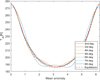 |
Fig. 2 Surface mean temperature Tav (ordinate) for a spherical analogue of (65803) Didymos, computed over one revolution about the Sun (mean anomaly ℓ at the abscissa). The orbital and physical parameters are taken from Table 1, and the coefficients of Tav up to degree nmax = 8 are obtained using our algorithm. The dashed black line shows the local equilibrium temperature Teq given by Eq. (46). |
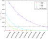 |
Fig. 3 Differences between consecutive degrees of approximation for four different values of e. The dashed line represents the accuracy of TIRI, and the solid lines are obtained through exponential fits that can be used to extrapolate an estimate of the required truncation degree for which the differences fall below the accuracy threshold. |
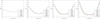 |
Fig. 4 Similar to Fig. 2, but now the orbital eccentricity e is varied for the sake of illustration (all other parameters, including the semi-major axis, have the nominal values): (i) e = 0.1 (top and left), (ii) e = 0.3 (top and right), (iii) e = 0.4 (bottom and left), and (iv) e = 0.5 (bottom and right). |
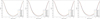 |
Fig. 5 Similar to Fig. 2, but now the thermal parameter Θ is varied for the sake of illustration (the nominal value e = 0.38 for the eccentricity is used here): (i) Θ = 0 (top and left), (ii) Θ = 0.033 (top and right), (iii) Θ = 0.07 (bottom and left), and (iv) Θ = 0.175 (bottom and right). The Θ = 0 solution for Tav is very close to the local equilibrium situation from (46), and increasing Θ values moves Tav away from equilibrium due to finite thermal relaxation. |
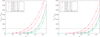 |
Fig. 6 Differences between consecutive degrees of approximation for varying e (left) and differences between the analytically computed local equilibrium temperature and the truncated average temperature obtained for Θ = 0 and varying e (right). The dashed lines represent the accuracy of TIRI, and the solid lines are obtained through exponential fits. |
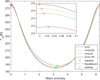 |
Fig. 7 Degree 8 mean temperature profiles for e = 0.38 and varied values of Θ (solid lines). The open circles indicate maxima (red) and minima (green) of Tav. The nested plot shows a zoom of the post-perihelion temperature profile. The higher Θ values result in a smaller difference between maximum and minimum Tav and a longer post-perihelion and -aphelion lag. |
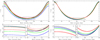 |
Fig. 8 Comparison between our formulation of the mean temperature Tav (degree 8 truncated series; dashed lines) and the mean value of the first (left panels) and fourth power (right panels) of the numerically determined temperature T(θ, ϕ; ℓ) defined by (49) (solid lines). The spherical body on a Didymos heliocentric orbit assumed and the four values of the thermal parameter used are Θ = 0 (black), Θ = 0.033 (blue), Θ = 0.07 (green), and Θ = 0.175 (red). |
5 Conclusions
We developed an analytical framework for determining the mean temperature Tav of a spherical body moving in an elliptic orbit about the Sun. The method uses power-series expansion in two parameters ζ = exp(ιℓ), which is equivalent to Fourier series in the mean anomaly ℓ, and ![Mathematical equation: $\[\beta=e /\left(1+\sqrt{1-e^{2}}\right)\]$](/articles/aa/full_html/2026/04/aa57911-25/aa57911-25-eq86.png) , where e is the orbital eccentricity. The resulting algorithm is well-behaved and was tested here to degree and order eight in the series expansion. This truncation allowed us to evaluate Tav for an eccentricity up to ≃0.4. In order to extend this range to higher eccentricity values, the approach can be efficiently extended to higher degrees and orders with no need to recompute the necessary coefficients determined so far. However, since the expansions used in our method use powers in eccentricity (or β), we expect a loss of convergence at the Laplace limit of e ~ 0.66.
, where e is the orbital eccentricity. The resulting algorithm is well-behaved and was tested here to degree and order eight in the series expansion. This truncation allowed us to evaluate Tav for an eccentricity up to ≃0.4. In order to extend this range to higher eccentricity values, the approach can be efficiently extended to higher degrees and orders with no need to recompute the necessary coefficients determined so far. However, since the expansions used in our method use powers in eccentricity (or β), we expect a loss of convergence at the Laplace limit of e ~ 0.66.
A possible future application of our results includes an analytical theory implementing seasonal and diurnal Yarkovsky effects, and their mutual interaction, for small Solar System bodies. With the mean temperature properly defined for eccentric orbits, this will generalize the results given by Vokrouhlický (1999), where the source of the coupling between the seasonal and diurnal Yarkovsky effects originated from a finite ratio of the revolution period about the Sun and the rotation period about the spin axis. Having formulated the mean temperature along an eccentric orbit, we will be able to analyse the interaction between the two variants of the Yarkovsky effect originating from the orbital eccentricity using an analytical approach.
Acknowledgements
RP and MM are grateful to the Italian Space Agency (ASI) for financial support through Agreement No. 2022-8-HH.0 in the context of ESA’s Hera mission. RP also acknowledges ASI’s support through the project “MONitoring ASTERoids” (grant 2022-33-HH.0). The work of DV was partially supported by the Czech Science Foudation (grant 25-16507S).
References
- Afonso, G. B., Gomes, R. S., & Florczak, M. A. 1995, Planet. Space Sci., 43, 787 [NASA ADS] [CrossRef] [Google Scholar]
- Bottke, W. F., Vokrouhlický, D., Rubincam, D. P., & Nesvorný, D. 2006, Annu. Rev. Earth Planet. Sci., 34, 157 [CrossRef] [Google Scholar]
- Breiter, S., Métris, G., & Vokrouhlický, D. 2004, Celest. Mech. Dyn. Astron., 88, 153 [Google Scholar]
- Čapek, D., & Vokrouhlický, D. 2004, Icarus, 172, 526 [Google Scholar]
- Čapek, D., & Vokrouhlický, D. 2005, in IAU Colloquium 197: Dynamics of Populations of Planetary Systems, eds. Z. Knežević, & A. Milani, 171 [Google Scholar]
- Čapek, D., & Vokrouhlický, D. 2010, A&A, 519, A75 [NASA ADS] [CrossRef] [EDP Sciences] [Google Scholar]
- Da Silva Fernandes, S. 1995, Celestial Mech. Dyn. Astron., 62, 305 [Google Scholar]
- Daly, R. T., Ernst, C. M., Barnouin, O. S., et al. 2023, Nature, 616, 443 [CrossRef] [Google Scholar]
- Delbó, M., Mueller, M., Emery, J. P., Rozitis, B., & Capria, M. T. 2015, in Asteroids IV, eds. P. Michel, F. E. DeMeo, & W. F. Bottke (University of Arizona Press Tucson), 107 [Google Scholar]
- Farinella, P., & Vokrouhlický, D. 1996, Planet. Space Sci., 44, 1551 [NASA ADS] [CrossRef] [Google Scholar]
- Farinella, P., Vokrouhlický, D., & Hartmann, W. K. 1998, Icarus, 132, 378 [NASA ADS] [CrossRef] [Google Scholar]
- Kuehrt, E. 1984, Icarus, 60, 512 [NASA ADS] [CrossRef] [Google Scholar]
- Michel, P., Küppers, M., Bagatin, A. C., et al. 2022, Planet. Sci. J., 3, 160 [NASA ADS] [CrossRef] [Google Scholar]
- Mysen, E. 2008, A&A, 484, 563 [NASA ADS] [CrossRef] [EDP Sciences] [Google Scholar]
- Naidu, S., Benner, L., Brozović, M., et al. 2020, Icarus, 348, 113777 [CrossRef] [Google Scholar]
- Novaković, B., & Fenucci, M. 2024, Icarus, 421, 116225 [CrossRef] [Google Scholar]
- Okada, T., Tanaka, S., Sakatani, N., et al. 2025, Space Sci. Rev., 221, 104 [Google Scholar]
- Peterson, C. 1976, Icarus, 29, 91 [NASA ADS] [CrossRef] [Google Scholar]
- Richardson, D. C., Agrusa, H. F., Barbee, B., et al. 2024, Planet. Sci. J., 5, 182 [NASA ADS] [CrossRef] [Google Scholar]
- Rivkin, A. S., Thomas, C. A., Wong, I., et al. 2023, Planet. Sci. J., 4, 214 [NASA ADS] [CrossRef] [Google Scholar]
- Rozitis, B., Green, S. F., Jackson, S. L., et al. 2024, Planet. Sci. J., 5, 66 [NASA ADS] [CrossRef] [Google Scholar]
- Rubincam, D. P. 1998, J. Geophys. Res., 103, 1725 [Google Scholar]
- Sekiya, M., & Shimoda, A. A. 2013, Planet. Space Sci., 84, 112 [Google Scholar]
- Sekiya, M., Shimoda, A. A., & Wakita, S. 2012, Planet. Space Sci., 60, 304 [NASA ADS] [CrossRef] [Google Scholar]
- Tisserand, F. 1894, Traité de mécanique céleste: Exposé de l’ensemble des théories relatives au mouvement de la lune, 3 (Gauthier-Villars) [Google Scholar]
- Tortora, P., Gramigna, E., Lasagni Manghi, R., et al. 2025, Space Sci. Rev., 221, 124 [Google Scholar]
- Vokrouhlický, D. 1998a, A&A, 335, 1093 [Google Scholar]
- Vokrouhlický, D. 1998b, A&A, 338, 353 [NASA ADS] [Google Scholar]
- Vokrouhlický, D. 1999, A&A, 344, 362 [NASA ADS] [Google Scholar]
- Vokrouhlický, D., & Farinella, P. 1999, AJ, 118, 3049 [CrossRef] [Google Scholar]
- Vokrouhlický, D., Bottke, W. F., Chesley, S. R., Scheeres, D. J., & Statler, T. S. 2015, in Asteroids IV, eds. P. Michel, F. E. DeMeo, & W. F. Bottke, 509 [Google Scholar]
Semi-analytical non-linear models were also developed (e.g., Vokrouhlický & Farinella 1999; Sekiya et al. 2012; Sekiya & Shimoda 2013), but, as in the case of the fully numerical approaches, the interpretation of their results is less obvious, and the CPU requirements are generally larger than in the case of a fully analytical treatment. These efforts include the remarkable paper by Peterson (1976), who treated the non-linearity of the boundary conditions analytically to the second order. As much as this work was quite ahead of its time, it still contained several approximations that were still to be removed: it only treated the diurnal variant of the Yarkovsky effect and assumed zero obliquity and a circular heliocentric orbit.
We also pondered the possibility of not developing Cn in series of powers in β, which might limit the applicability of the method in orbital eccentricity. However, attempts to solve Cn directly from (13) by only comparing powers in ζ ran into algebraic difficulties that we were unable to solve.
More accurately, the R′ dependence of the coefficient Cn transitions at ![Mathematical equation: $\[\sqrt{n} R^{\prime} \simeq 1\]$](/articles/aa/full_html/2026/04/aa57911-25/aa57911-25-eq99.png) , but the lowest values n generally dominate.
, but the lowest values n generally dominate.
Appendix A Symbols and notation
| Constants and parameters: | |
| nmax | maximum degree of truncation |
| σ | Stefan–Boltzmann constant |
| ρ | density |
| C | thermal capacity |
| K | thermal conductivity |
| Γ | thermal inertia |
| α | absorption coefficient |
| ϵ | emissivity |
| R | effective radius of the body |
| Θ | thermal parameter |
| Θn | auxiliary thermal parameter defined by ![Mathematical equation: $\[\Theta_{n}=\sqrt{n} \Theta\]$](/articles/aa/full_html/2026/04/aa57911-25/aa57911-25-eq87.png) , with n = 1, ..., nmax , with n = 1, ..., nmax
|
| hs | penetration depth of the seasonal thermal wave |
| n | mean motion |
| a | semimajor axis |
| e | eccentricity |
| eL | Laplace limit |
| β | ![Mathematical equation: $\[\beta=e /\left(1+\sqrt{1-e^{2}}\right)\]$](/articles/aa/full_html/2026/04/aa57911-25/aa57911-25-eq88.png) |
| Fa | solar radiation flux at distance equal to the semimajor axis |
| Ta | reference temperature defined by ![Mathematical equation: $\[\epsilon \sigma T_{a}^{4}=\alpha F_{a}\]$](/articles/aa/full_html/2026/04/aa57911-25/aa57911-25-eq89.png)
|
| Variables: | |
| r | radial position with respect to the body centre |
| r′ | radial position scaled by hs |
| d | distance from the Sun |
| t | time |
| ℓ | mean anomaly |
| ζ | time-related variable, ζ = eiℓ |
| T | temperature |
| Tav | mean temperature |
![Mathematical equation: $\[T_{a v}^{\prime}\]$](/articles/aa/full_html/2026/04/aa57911-25/aa57911-25-eq90.png) |
mean temperature scaled by Ta |
| Teq | local equilibrium temperature obtained from ![Mathematical equation: $\[T_{\text {av }}^{\prime 4}=\overline{\mathcal{E}}^{\prime}\]$](/articles/aa/full_html/2026/04/aa57911-25/aa57911-25-eq91.png)
|
| ΔT | temperature variation with respect to the average value |
| ℰ | insolation |
![Mathematical equation: $\[\bar{T}\]$](/articles/aa/full_html/2026/04/aa57911-25/aa57911-25-eq92.png) |
mean surface temperature |
![Mathematical equation: $\[\overline{\mathcal{E}}^{\prime}\]$](/articles/aa/full_html/2026/04/aa57911-25/aa57911-25-eq93.png) |
average insolation scaled by the reference flux Fa |
| xn | ![Mathematical equation: $\[x_{n}=\sqrt{n / 2} R^{\prime}\]$](/articles/aa/full_html/2026/04/aa57911-25/aa57911-25-eq94.png) |
| zn | ![Mathematical equation: $\[z_{n}=\sqrt{-\iota n} ~r^{\prime}\]$](/articles/aa/full_html/2026/04/aa57911-25/aa57911-25-eq95.png) |
| Coefficients: | |
| an | Hansen coefficients |
| Cn | coefficients of the expansion in terms of ζ |
| Cnk | coefficients of the expansion of Cn in terms of β |
| Functions: | |
| j0 | zeroth spherical Bessel function of the first kind |
| ψn | function defined by (z/j0(z)) dz(j0(z)|z=Zn |
![Mathematical equation: $\[G_{n}^{+}, G_{n}^{-}, F_{n}\]$](/articles/aa/full_html/2026/04/aa57911-25/aa57911-25-eq96.png) |
auxiliary functions |
Appendix B Coefficients Cnk up to degree and order eight
Here we provide explicit formulas for coefficients Cnk up to degree and order eight for the large-body limit (R′ → ∞). We introduce the following quantities
![Mathematical equation: $\[\begin{aligned}\Theta_n= & \sqrt{n} \Theta \qquad \text { and } \qquad Z_n=\frac{1+\Theta_n / 2-i \Theta_n / 2}{\sqrt{2}\left(1+\Theta_n+\Theta_n^2 / 2\right),} \qquad \text { with which we obtain: } \\C_{11}= & Z_1 / 2 \qquad\quad C_{02}=\left(12 C_{-11} C_{11}-1\right) /(2 \sqrt{2}) \qquad\quad C_{22}=Z_2\left(125-3 C_{11}^2\right) \qquad\quad C_{33}=Z_3\left(13-8 \sqrt{2} C_{11}^3-24 C_{11} C_{22}\right) / 4 \\C_{13}= & Z_1\left[1-24 C_{-11}\left(\sqrt{2} C_{11}^2+C_{22}\right)-24 C_{11} C_{02}\right] / 4 \qquad\quad C_{44}=Z_4\left(103-12 C_{11}^4-72 \sqrt{2} C_{11}^2 C_{22}-36 C_{22}^2-72 C_{11} C_{33}\right) / 12 \\C_{24}= & -Z_2\left[11+36 C_{11} C_{13}+12 C_{-11}\left(2 C_{11}^3+6 \sqrt{2} C_{11} C_{22}+3 C_{33}\right)+36 \sqrt{2} C_{11}^2 C_{02}+36 C_{22} C_{02}\right] / 6 \\C_{04}= & \left(1-12 C_{-13} C_{11}-12 \sqrt{2} C_{-22} C_{11}^2-12 C_{-11}^2 C_{11}^2-12 C_{-11} C_{13}-12 C_{-22} C_{22}-12 \sqrt{2} C_{-11}^2 C_{22}-24 \sqrt{2} C_{-11} C_{11} C_{02}-6 C_{02}^2\right) /(2 \sqrt{2}) \\C_{55}= & \left.Z_5\left(1097-192 C_{11}^3 C_{22}-288 \sqrt{2} C_{11}^2 C_{33}-288 C_{22} C_{33}-288 C_{11}\left(\sqrt{2} C_{22}^2+C_{44}\right)\right) Z_5\right) / 48 \\C_{35}= & -Z_3\left\{181+96 C_{13} C_{22}+96 \sqrt{2} C_{-11} C_{22}^2+96 C_{11}^2\left(\sqrt{2} C_{13}+2 C_{-11} C_{22}\right)+96 C_{-11} C_{44}+64 C_{11}^3 C_{02}+96 C_{33} C_{02}\right. \\& \left.+96 C_{11}\left[C_{24}+2 \sqrt{2}\left(C_{-11} C_{33}+C_{22} C_{02}\right)\right]\right\} / 16\\C_{15}= & Z_1\left[23-288 \sqrt{2} C_{-11} C_{11} C_{13}-288 C_{-11}^2 C_{11} C_{22}-144 C_{-13}\left(\sqrt{2} C_{11}^2+C_{22}\right)-144 C_{-11} C_{24}-144 \sqrt{2} C_{-11}^2 C_{33}\right. \\& \left.-48 C_{-22}\left(2 C_{11}^3+6 \sqrt{2} C_{11} C_{22}+3 C_{33}\right)-288 C_{-11} C_{11}^2 C_{02}-144 C_{13} C_{02}-288 \sqrt{2} C_{-11} C_{22} C_{02}-144 \sqrt{2} C_{11} C_{02}^2-144 C_{11} C_{04}\right] / 24 \\C_{66}= & Z_6\left[1223-40 \sqrt{2} C_{22}^3-80 C_{11}^3 C_{33}-60 C_{33}^2-120 C_{22} C_{44}-120 C_{11}^2\left(C_{22}^2+\sqrt{2} C_{44}\right)-120 C_{11}\left(2 \sqrt{2} C_{22} C_{33}+C_{55}\right)\right] / 20 \\C_{46}= & -Z_4\left\{1417+120 C_{11}^3 C_{13}+180 C_{13} C_{33}+180 C_{22}\left(C_{24}+2 \sqrt{2} C_{-11} C_{33}\right)+180 C_{-11} C_{55}+180 \sqrt{2} C_{22}^2 C_{02}+180 C_{44} C_{02}\right. \\& \left.+180 C_{11}^2\left(\sqrt{2} C_{24}+2 C_{-11} C_{33}+2 C_{22} C_{02}\right)+180 C_{11}\left[2 \sqrt{2} C_{13} C_{22}+C_{35}+2 C_{-11}\left(C_{22}^2+\sqrt{2} C_{44}\right)+2 \sqrt{2} C_{33} C_{02}\right]\right\} / 30 \\C_{26}= & Z_2\left\{19-9 C_{13}^2-18 C_{11} C_{15}-36 C_{-22} C_{11}^2 C_{22}-18 \sqrt{2} C_{-22} C_{22}^2-36 \sqrt{2} C_{-22} C_{11} C_{33}-6 C_{-13}\left(2 C_{11}^3+6 \sqrt{2} C_{11} C_{22}+3 C_{33}\right)\right. \\& -18 C_{-22} C_{44}-18 C_{-11}^2\left(C_{22}^2+2 C_{11} C_{33}+\sqrt{2} C_{44}\right)-36 \sqrt{2} C_{11} C_{13} C_{02}-18 C_{24} C_{02}-18 C_{11}^2 C_{02}^2-18 \sqrt{2} C_{22} C_{02}^2 \\& \left.-18 C_{-11}\left[2 C_{11}^2 C_{13}+2 \sqrt{2} C_{13} C_{22}+C_{35}+2 \sqrt{2} C_{33} C_{02}+2 C_{11}\left(\sqrt{2} C_{24}+2 C_{22} C_{02}\right)\right]-18 \sqrt{2} C_{11}^2 C_{04}-18 C_{22} C_{04}\right\} / 3\\C_{06}= & \left(1-12 C_{-15} C_{11}-12 \sqrt{2} C_{-24} C_{11}^2-24 C_{-11} C_{-13} C_{11}^2-8 C_{-33} C_{11}^3-12 C_{-13} C_{13}-24 \sqrt{2} C_{-22} C_{11} C_{13}-24 C_{-11}^2 C_{11} C_{13}\right. \\& -12 C_{-11} C_{15}-12 C_{-24} C_{22}-24 \sqrt{2} C_{-11} C_{-13} C_{22}-24 \sqrt{2} C_{-33} C_{11} C_{22}-48 C_{-22} C_{-11} C_{11} C_{22}-12 C_{-22} C_{24}-12 \sqrt{2} C_{-11}^2 C_{24} \\& -12 C_{-33} C_{33}+24 \sqrt{2} C_{-22} C_{-11} C_{33}-8 C_{-11}^3 C_{33}-24 \sqrt{2} C_{-13} C_{11} C_{02}-24 C_{-22} C_{11}^2 C_{02}-24 \sqrt{2} C_{-11} C_{13} C_{02}-24 \sqrt{2} C_{-22} C_{22} C_{02} \\& \left.-24 C_{-11}^2 C_{22} C_{02}-24 C_{-11} C_{11} C_{02}^2-4 \sqrt{2} C_{02}^3-24 \sqrt{2} C_{-11} C_{11} C_{04}-12 C_{02} C_{04}\right) /(2 \sqrt{2}) \\C_{77}= & Z_7\left\{47273 / 288-6 \sqrt{2} C_{22}^2 C_{33}-4 C_{11}^3 C_{44}-6 C_{33} C_{44}-6 C_{22} C_{55}\right. \\& \left.-6 C_{11}^2\left(2 C_{22} C_{33}+\sqrt{2} C_{55}\right)-2 C_{11}\left[2 C_{22}^3+6 \sqrt{2} C_{22} C_{44}+3\left(\sqrt{2} C_{33}^2+C_{66}\right)\right]\right\} \\C_{57}= & -Z_5\left\{49531+1152 C_{-11} C_{22}^3+1152 C_{11}^3 C_{24}+1728 C_{24} C_{33}+1728 \sqrt{2} C_{-11} C_{33}^2+1728 C_{22} C_{35}+3456 \sqrt{2} C_{-11} C_{22} C_{44}\right. \\& +1728 C_{13}\left(\sqrt{2} C_{22}^2+C_{44}\right)+1728 C_{-11} C_{66}+3456 \sqrt{2} C_{22} C_{33} C_{02}+1728 C_{55} C_{02}+1728 C_{11}^2\left(2 C_{13} C_{22}+\sqrt{2} C_{35}+2 C_{-11} C_{44}\right. \\& \left.\left.+2 C_{33} C_{02}\right)+1728 C_{11}\left[2 \sqrt{2} C_{13} C_{33}+2 C_{22}\left(\sqrt{2} C_{24}+2 C_{-11} C_{33}\right)+C_{46}+2 \sqrt{2} C_{-11} C_{55}+2 C_{22}^2 C_{02}+2 \sqrt{2} C_{44} C_{02}\right]\right\} / 288\\C_{37}= & Z_3\left\{1267-192 C_{15} C_{22}-192 \sqrt{2} C_{-13} C_{22}^2-192 C_{13} C_{24}-384 \sqrt{2} C_{-11} C_{22} C_{24}-384 \sqrt{2} C_{-11} C_{13} C_{33}-384 \sqrt{2} C_{-22} C_{22} C_{33}\right. \\& -384 C_{-11}^2 C_{22} C_{33}-192 C_{-13} C_{44}-192 C_{-11} C_{46}-192 C_{-22} C_{55}-192 \sqrt{2} C_{-11}^2 C_{55}-384 \sqrt{2} C_{13} C_{22} C_{02}-384 C_{-11} C_{22}^2 C_{02} \\& -192 C_{35} C_{02}-384 \sqrt{2} C_{-11} C_{44} C_{02}-192 \sqrt{2} C_{33} C_{02}^2-192 C_{11}^2\left[\sqrt{2} C_{15}+2\left(C_{-13} C_{22}+C_{-11} C_{24}+C_{-22} C_{33}+C_{13} C_{02}\right)\right] \\& -128 C_{11}^3 C_{04}-192 C_{33} C_{04}-192 C_{11}\left[\sqrt{2} C_{13}^2+4 C_{-11} C_{13} C_{22}+C_{26}+2 \sqrt{2} C_{-13} C_{33}+2 \sqrt{2} C_{-11} C_{35}+2 C_{-11}^2 C_{44}\right. \\& \left.\left.+2 C_{-22}\left(C_{22}^2+\sqrt{2} C_{44}\right)+2 \sqrt{2} C_{24} C_{02}+4 C_{-11} C_{33} C_{02}+2 C_{22} C_{02}^2+2 \sqrt{2} C_{22} C_{04}\right]\right\} / 32 \\C_{17}= & -Z_1\left(73+3456 \sqrt{2} C_{-13} C_{11} C_{13}+3456 C_{-22} C_{11}^2 C_{13}+1728 \sqrt{2} C_{-11} C_{13}^2+3456 \sqrt{2} C_{-11} C_{11} C_{15}\right. \\& +6912 C_{-11} C_{-13} C_{11} C_{22}+3456 C_{-33} C_{11}^2 C_{22}+3456 \sqrt{2} C_{-22} C_{13} C_{22}+3456 C_{-11}^2 C_{13} C_{22}+1728 \sqrt{2} C_{-33} C_{22}^2 \\& +3456 C_{-22} C_{-11} C_{22}^2+1728 C_{-15}\left(\sqrt{2} C_{11}^2+C_{22}\right)+1728 C_{-13} C_{24}+3456 \sqrt{2} C_{-22} C_{11} C_{24}+3456 C_{-11}^2 C_{11} C_{24} \\& +1728 C_{-11} C_{26}+3456 \sqrt{2} C_{-11} C_{-13} C_{33}+3456 \sqrt{2} C_{-33} C_{11} C_{33}+6912 C_{-22} C_{-11} C_{11} C_{33}+576 C_{-24}\left(2 C_{11}^3+6 \sqrt{2} C_{11} C_{22}\right. \\& \left.+3 C_{33}\right)+1728 C_{-22} C_{35}+1728 \sqrt{2} C_{-11}^2 C_{35}+1728 C_{-33} C_{44}+3456 \sqrt{2} C_{-22} C_{-11} C_{44}+1152 C_{-11}^3 C_{44}+3456 C_{-13} C_{11}^2 C_{02} \\& +6912 C_{-11} C_{11} C_{13} C_{02}+1728 C_{15} C_{02}+3456 \sqrt{2} C_{-13} C_{22} C_{02}+6912 C_{-22} C_{11} C_{22} C_{02}+3456 \sqrt{2} C_{-11} C_{24} C_{02} \\& +3456 \sqrt{2} C_{-22} C_{33} C_{02}+3456 C_{-11}^2 C_{33} C_{02}+1728 \sqrt{2} C_{13} C_{02}^2+3456 C_{-11} C_{22} C_{02}^2+1152 C_{11} C_{02}^3+3456 C_{-11} C_{11}^2 C_{04} \\& +1728 C_{13} C_{04}+3456 \sqrt{2} C_{-11} C_{22} C_{04}+3456 \sqrt{2} C_{11} C_{02} C_{04}+1728 C_{11} C_{06}) / 288 \\C_{88}= & Z_8\left[556403 / 1260-C_{22}^4-3 C_{44}^2-6 C_{22}^2\left(2 C_{11} C_{33}+\sqrt{2} C_{44}\right)-4 C_{11}^3 C_{55}-6 C_{33} C_{55}-6 C_{22}\left(\sqrt{2} C_{33}^2+2 C_{11}^2 C_{44}\right.\right. \\& \left.\left.+2 \sqrt{2} C_{11} C_{55}+C_{66}\right)-6 C_{11}^2\left(C_{33}^2+\sqrt{2} C_{66}\right)-6 C_{11}\left(2 \sqrt{2} C_{33} C_{44}+C_{77}\right)\right] \\C_{68}= & -Z_6\left\{40861+420 C_{22}^2\left(\sqrt{2} C_{24}+2 C_{-11} C_{33}\right)+280 C_{11}^3 C_{35}+420 C_{33} C_{35}+420 C_{24} C_{44}+840 \sqrt{2} C_{-11} C_{33} C_{44}\right. \\& +420 C_{13} C_{55}+420 C_{-11} C_{77}+280 C_{22}^3 C_{02}+420 \sqrt{2} C_{33}^2 C_{02}+420 C_{66} C_{02}+420 C_{11}^2\left(2 C_{22} C_{24}+2 C_{13} C_{33}+\sqrt{2} C_{46}\right. \\& \left.+2 C_{-11} C_{55}+2 C_{44} C_{02}\right)+420 C_{11}\left[2 \sqrt{2} C_{24} C_{33}+2 C_{-11} C_{33}^2+2 \sqrt{2} C_{22} C_{35}+4 C_{-11} C_{22} C_{44}+2 C_{13}\left(C_{22}^2+\sqrt{2} C_{44}\right)+C_{57}\right. \\& \left.\left.+2 \sqrt{2} C_{-11} C_{66}+4 C_{22} C_{33} C_{02}+2 \sqrt{2} C_{55} C_{02}\right]+420 C_{22}\left[2 \sqrt{2} C_{13} C_{33}+C_{46}+2 \sqrt{2}\left(C_{-11} C_{55}+C_{44} C_{02}\right)\right]\right\} / 70 \\C_{48}= & Z_4\left\{18037-360 C_{11}^3 C_{15}-540 \sqrt{2} C_{13}^2 C_{22}-360 C_{-22} C_{22}^3-270 C_{24}^2-540 C_{22} C_{26}-540 C_{15} C_{33}-1080 \sqrt{2} C_{-13} C_{22} C_{33}\right. \\& -1080 \sqrt{2} C_{-11} C_{24} C_{33}-540 \sqrt{2} C_{-22} C_{33}^2-540 C_{-11}^2 C_{33}^2-1080 \sqrt{2} C_{-11} C_{22} C_{35}-1080 \sqrt{2} C_{-22} C_{22} C_{44}-1080 C_{-11}^2 C_{22} C_{44} \\& -540 C_{-13} C_{55}-540 C_{-11} C_{57}-540 C_{-22} C_{66}-540 \sqrt{2} C_{-11}^2 C_{66}-1080 \sqrt{2} C_{22} C_{24} C_{02}-2160 C_{-11} C_{22} C_{33} C_{02}-540 C_{46} C_{02} \\& -1080 \sqrt{2} C_{-11} C_{55} C_{02}-540 C_{22}^2 C_{02}^2-540 \sqrt{2} C_{44} C_{02}^2-540 C_{13}\left[C_{35}+2 C_{-11}\left(C_{22}^2+\sqrt{2} C_{44}\right)+2 \sqrt{2} C_{33} C_{02}\right]-540 \sqrt{2} C_{22}^2 C_{04} \\& -540 C_{44} C_{04}-540 C_{11}\left[2 \sqrt{2} C_{15} C_{22}+2 \sqrt{2} C_{13} C_{24}+4 C_{-11} C_{22} C_{24}+4 C_{-11} C_{13} C_{33}+4 C_{-22} C_{22} C_{33}+C_{37}+2 C_{-13}\left(C_{22}^2\right.\right. \\& \left.\left.+\sqrt{2} C_{44}\right)+2 \sqrt{2} C_{-11} C_{46}+2 \sqrt{2} C_{-22} C_{55}+2 C_{-11}^2 C_{55}+4 C_{13} C_{22} C_{02}+2 \sqrt{2} C_{35} C_{02}+4 C_{-11} C_{44} C_{02}+2 C_{33} C_{02}^2+2 \sqrt{2} C_{33} C_{04}\right] \\& \left.-540 C_{11}^2\left[C_{13}^2+\sqrt{2} C_{26}+2\left(C_{-13} C_{33}+C_{-11} C_{35}+C_{-22} C_{44}+C_{24} C_{02}+C_{22} C_{04}\right)\right]\right\} / 90\\C_{28}= & -Z_2\left\{1127+1080 C_{-11} C_{11} C_{13}^2+1080 C_{-11} C_{11}^2 C_{15}+40 C_{13} C_{15}+540 C_{11} C_{17}+1080 C_{-24} C_{11}^2 C_{22}\right. \\& +160 C_{-22} C_{11} C_{13} C_{22}+1080 \sqrt{2} C_{-11} C_{15} C_{22}+540 \sqrt{2} C_{-24} C_{22}^2+1080 C_{-33} C_{11} C_{22}^2+1080 C_{-22} C_{11}^2 C_{24} \\& +1080 \sqrt{2} C_{-11} C_{13} C_{24}+1080 \sqrt{2} C_{-22} C_{22} C_{24}+1080 C_{-11}^2 C_{22} C_{24}+1080 \sqrt{2} C_{-11} C_{11} C_{26}+1080 \sqrt{2} C_{-24} C_{11} C_{33} \\& +1080 C_{-33} C_{11}^2 C_{33}+1080 \sqrt{2} C_{-22} C_{13} C_{33}+1080 C_{-11}^2 C_{13} C_{33}+1080 \sqrt{2} C_{-33} C_{22} C_{33}+2160 C_{-22} C_{-11} C_{22} C_{33} \\& +180 C_{-15}\left(2 C_{11}^3+6 \sqrt{2} C_{11} C_{22}+3 C_{33}\right)+1080 \sqrt{2} C_{-22} C_{11} C_{35}+1080 C_{-11}^2 C_{11} C_{35}+540 C_{-11} C_{37}+540 C_{-24} C_{44} \\& +1080 \sqrt{2} C_{-33} C_{11} C_{44}+2160 C_{-22} C_{-11} C_{11} C_{44}+540 C_{-22} C_{46}+540 \sqrt{2} C_{-11}^2 C_{46}+540 C_{-33} C_{55}+1080 \sqrt{2} C_{-22} C_{-11} C_{55} \\& +360 C_{-11}^3 C_{55}+540 \sqrt{2} C_{13}^2 C_{02}+1080 \sqrt{2} C_{11} C_{15} C_{02}+2160 C_{-11} C_{13} C_{22} C_{02}+1080 C_{-22} C_{22}^2 C_{02}+2160 C_{-11} C_{11} C_{24} C_{02} \\& +540 C_{26} C_{02}+2160 C_{-22} C_{11} C_{33} C_{02}+1080 \sqrt{2} C_{-11} C_{35} C_{02}+1080 \sqrt{2} C_{-22} C_{44} C_{02}+1080 C_{-11}^2 C_{44} C_{02}+1080 C_{11} C_{13} C_{02}^2 \\& +540 \sqrt{2} C_{24} C_{02}^2+1080 C_{-11} C_{33} C_{02}^2+360 C_{22} C_{02}^3+540 C_{-13}\left[2 C_{11}^2 C_{13}+2 \sqrt{2} C_{13} C_{22}+2 C_{-11} C_{22}^2+C_{35}+2 \sqrt{2} C_{-11} C_{44}\right. \\& \left.+2 \sqrt{2} C_{33} C_{02}+2 C_{11}\left(\sqrt{2} C_{24}+2 C_{-11} C_{33}+2 C_{22} C_{02}\right)\right]+1080 \sqrt{2} C_{11} C_{13} C_{04}+2160 C_{-11} C_{11} C_{22} C_{04}+540 C_{24} C_{04} \\& +1080 \sqrt{2} C_{-11} C_{33} C_{04}+1080 C_{11}^2 C_{02} C_{04}+1080 \sqrt{2} C_{22} C_{02} C_{04}+540 \sqrt{2} C_{11}^2 C_{06}+540 C_{22} C_{06}\} / 90\\C_{08}= & \left(1-12 C_{-17} C_{11}-12 \sqrt{2} C_{-26} C_{11}^2-12 C_{-13}^2 C_{11}^2-24 C_{-11} C_{-15} C_{11}^2-8 C_{-35} C_{11}^3-12 C_{-15} C_{13}-24 \sqrt{2} C_{-24} C_{11} C_{13}\right. \\& -48 C_{-11} C_{-13} C_{11} C_{13}-24 C_{-33} C_{11}^2 C_{13}-12 \sqrt{2} C_{-22} C_{13}^2-12 C_{-11}^2 C_{13}^2-12 C_{-13} C_{15}-24 \sqrt{2} C_{-22} C_{11} C_{15}-24 C_{-11}^2 C_{11} C_{15} \\& -12 C_{-11} C_{17}-12 C_{-26} C_{22}-12 \sqrt{2} C_{-13}^2 C_{22}-24 \sqrt{2} C_{-11} C_{-15} C_{22}-24 \sqrt{2} C_{-35} C_{11} C_{22}-48 C_{-24} C_{-11} C_{11} C_{22} \\& -48 C_{-22} C_{-13} C_{11} C_{22}-24 C_{-44} C_{11}^2 C_{22}-4 \sqrt{2} C_{-33} C_{13} C_{22}-48 C_{-22} C_{-11} C_{13} C_{22}-12 \sqrt{2} C_{-44} C_{22}^2-12 C_{-22}^2 C_{22}^2-24 C_{-33} C_{-11} C_{22}^2 \\& -12 C_{-24} C_{24}-24 \sqrt{2} C_{-11} C_{-13} C_{24}-24 \sqrt{2} C_{-33} C_{11} C_{24}-48 C_{-22} C_{-11} C_{11} C_{24}-12 C_{-22} C_{26}-12 \sqrt{2} C_{-11}^2 C_{26}-12 C_{-35} C_{33} \\& -24 \sqrt{2} C_{-24} C_{-11} C_{33}-24 \sqrt{2} C_{-22} C_{-13} C_{33}-24 C_{-11}^2 C_{-13} C_{33}-24 \sqrt{2} C_{-44} C_{11} C_{33}-24 C_{-22}^2 C_{11} C_{33}-48 C_{-33} C_{-11} C_{11} C_{33} \\& -12 C_{-33} C_{35}-24 \sqrt{2} C_{-22} C_{-11} C_{35}-8 C_{-11}^3 C_{35}-12 C_{-44} C_{44}-12 \sqrt{2} C_{-22}^2 C_{44}-24 \sqrt{2} C_{-33} C_{-11} C_{44}-24 C_{-22} C_{-11}^2 C_{44} \\& -24 \sqrt{2} C_{-15} C_{11} C_{02}-24 C_{-24} C_{11}^2 C_{02}-24 \sqrt{2} C_{-13} C_{13} C_{02}-48 C_{-22} C_{11} C_{13} C_{02}-24 \sqrt{2} C_{-11} C_{15} C_{02}-24 \sqrt{2} C_{-24} C_{22} C_{02} \\& -48 C_{-11} C_{-13} C_{22} C_{02}-48 C_{-33} C_{11} C_{22} C_{02}-24 \sqrt{2} C_{-22} C_{24} C_{02}-24 C_{-11}^2 C_{24} C_{02}-24 \sqrt{2} C_{-33} C_{33} C_{02}-48 C_{-22} C_{-11} C_{33} C_{02} \\& -24 C_{-13} C_{11} C_{02}^2-24 C_{-11} C_{13} C_{02}^2-24 C_{-22} C_{22} C_{02}^2-2 C_{02}^4-24 \sqrt{2} C_{-13} C_{11} C_{04}-24 C_{-22} C_{11}^2 C_{04}-24 \sqrt{2} C_{-11} C_{13} C_{04} \\& \left.-24 \sqrt{2} C_{-22} C_{22} C_{04}-24 C_{-11}^2 C_{22} C_{04}-48 C_{-11} C_{11} C_{02} C_{04}-12 \sqrt{2} C_{02}^2 C_{04}-6 C_{04}^2-24 \sqrt{2} C_{-11} C_{11} C_{06}-2 C_{02} C_{06}\right) /(2 \sqrt{2})\end{aligned}\]$](/articles/aa/full_html/2026/04/aa57911-25/aa57911-25-eq97.png)
The above formulas can be reproduced using the Mathematica® script available in the supplementary material of this paper, or at https://github.com/bubberio/average_temperature_formulas.
Remark. The above formulas are also valid for the small body limit (R′ → 0) when
![Mathematical equation: $\[Z_n=\frac{1}{\sqrt{2}} \quad V_n \neq 0\]$](/articles/aa/full_html/2026/04/aa57911-25/aa57911-25-eq98.png) is used. This is because in practice the case of the small body limit is equivalent to the case in which Θ = 0.
is used. This is because in practice the case of the small body limit is equivalent to the case in which Θ = 0.
All Tables
All Figures
|
Fig. 1 Flow chart for determining coefficients Cnk up to nmax = 4. The algorithm proceeds in the order indicated by the blue arrows. The shaded areas show that when nmax is increased to 5, most of the needed coefficients are already known, and it suffices to only compute three new ones: C15, C35, and C55. |
| In the text | |
|
Fig. 2 Surface mean temperature Tav (ordinate) for a spherical analogue of (65803) Didymos, computed over one revolution about the Sun (mean anomaly ℓ at the abscissa). The orbital and physical parameters are taken from Table 1, and the coefficients of Tav up to degree nmax = 8 are obtained using our algorithm. The dashed black line shows the local equilibrium temperature Teq given by Eq. (46). |
| In the text | |
|
Fig. 3 Differences between consecutive degrees of approximation for four different values of e. The dashed line represents the accuracy of TIRI, and the solid lines are obtained through exponential fits that can be used to extrapolate an estimate of the required truncation degree for which the differences fall below the accuracy threshold. |
| In the text | |
|
Fig. 4 Similar to Fig. 2, but now the orbital eccentricity e is varied for the sake of illustration (all other parameters, including the semi-major axis, have the nominal values): (i) e = 0.1 (top and left), (ii) e = 0.3 (top and right), (iii) e = 0.4 (bottom and left), and (iv) e = 0.5 (bottom and right). |
| In the text | |
|
Fig. 5 Similar to Fig. 2, but now the thermal parameter Θ is varied for the sake of illustration (the nominal value e = 0.38 for the eccentricity is used here): (i) Θ = 0 (top and left), (ii) Θ = 0.033 (top and right), (iii) Θ = 0.07 (bottom and left), and (iv) Θ = 0.175 (bottom and right). The Θ = 0 solution for Tav is very close to the local equilibrium situation from (46), and increasing Θ values moves Tav away from equilibrium due to finite thermal relaxation. |
| In the text | |
|
Fig. 6 Differences between consecutive degrees of approximation for varying e (left) and differences between the analytically computed local equilibrium temperature and the truncated average temperature obtained for Θ = 0 and varying e (right). The dashed lines represent the accuracy of TIRI, and the solid lines are obtained through exponential fits. |
| In the text | |
|
Fig. 7 Degree 8 mean temperature profiles for e = 0.38 and varied values of Θ (solid lines). The open circles indicate maxima (red) and minima (green) of Tav. The nested plot shows a zoom of the post-perihelion temperature profile. The higher Θ values result in a smaller difference between maximum and minimum Tav and a longer post-perihelion and -aphelion lag. |
| In the text | |
|
Fig. 8 Comparison between our formulation of the mean temperature Tav (degree 8 truncated series; dashed lines) and the mean value of the first (left panels) and fourth power (right panels) of the numerically determined temperature T(θ, ϕ; ℓ) defined by (49) (solid lines). The spherical body on a Didymos heliocentric orbit assumed and the four values of the thermal parameter used are Θ = 0 (black), Θ = 0.033 (blue), Θ = 0.07 (green), and Θ = 0.175 (red). |
| In the text | |
Current usage metrics show cumulative count of Article Views (full-text article views including HTML views, PDF and ePub downloads, according to the available data) and Abstracts Views on Vision4Press platform.
Data correspond to usage on the plateform after 2015. The current usage metrics is available 48-96 hours after online publication and is updated daily on week days.
Initial download of the metrics may take a while.