| Issue |
A&A
Volume 708, April 2026
|
|
|---|---|---|
| Article Number | A72 | |
| Number of page(s) | 14 | |
| Section | Extragalactic astronomy | |
| DOI | https://doi.org/10.1051/0004-6361/202558063 | |
| Published online | 26 March 2026 | |
The nuclear star cluster of M 74: A fossil record of the very early stages of a star-forming galaxy
1
Instituto de Astrofísica de Canarias, Calle Vía Láctea s/n, E-38205 La Laguna, Tenerife, Spain
2
Departamento de Astrofísica, Universidad de La Laguna, Avenida Astrofísico Francisco Sánchez s/n, E-38206 La Laguna, Spain
3
Max-Planck-Institut für Astronomie, Königstuhl 17, D-69117 Heidelberg, Germany
4
Université Côte d’Azur, Observatoire de la Côte d’Azur, CNRS, Laboratoire Lagrange, 06000 Nice, France
5
Department of Physics and Astronomy, University of Wyoming, Laramie, WY 82071, USA
6
Research School of Astronomy and Astrophysics, Australian National University, Weston Creek, ACT 2611, Australia
7
Universität Heidelberg, Institut für Theoretische Astrophysik, Albert-Ueberle-Str 2, D-69120 Heidelberg, Germany
8
Universität Heidelberg, Interdisziplinäres Zentrum für Wissenschaftliches Rechnen, Im Neuenheimer Feld 205, D-69120 Heidelberg, Germany
9
Observatorio Astronómico Nacional (IGN), C/Alfonso XII, 3, E-28014 Madrid, Spain
10
UK ALMA Regional Centre Node, Jodrell Bank Centre for Astrophysics, University of Manchester, Oxford Road, Manchester M13 9PL, UK
11
Astronomy Department, The Ohio State University, Columbus, Ohio, USA
12
Center for Cosmology and Astro-Particle Physics, The Ohio State University, Columbus, Ohio, USA
★ Corresponding author: This email address is being protected from spambots. You need JavaScript enabled to view it.
Received:
11
November
2025
Accepted:
2
March
2026
Abstract
Nuclear star clusters (NSC) are dense and compact stellar systems with sizes of a few parsecs located at galactic centers. Their properties and formation mechanisms seem to be tightly linked to the evolution of the host galaxy, with potentially different formation channels for late- and early-type galaxies (LTGs and ETGs). While most observations target ETGs, here we focus on the NSC in M 74 (NGC 628), a relatively massive and gas-rich star-forming spiral galaxy included in the PHANGS survey. We analyzed the central arc minute of the PHANGS-MUSE mosaic, in which the NSC is not spatially resolved. We analyzed the NSC stellar populations in a point spread function (PSF) aperture and compared it to the host galaxy. Within the PSF size, the NSC is contaminated by the host galaxy light. We performed a two-dimensional spectro-photometric decomposition of the MUSE cube, employing a modified version of the C2D code, to disentangle the NSC from its host. This method provided different data cubes for the NSC and the host galaxy, allowing for their comparison in a PSF aperture, as well as a spatially resolved analysis of the host. Our results show a very old and metal-poor NSC, in contrast to the surrounding regions. While similar properties have been found in NSCs hosted by galaxies of different masses and/or morphological types from M 74, they are somewhat unexpected for a relatively massive star-forming spiral galaxy. The spatially resolved stellar populations of the host galaxy display much younger (light-weighted) ages and higher metallicities, especially in the central region (∼500 pc) surrounding the NSC. This suggests that this NSC formed a long time ago and evolved passively until today without any further growth. No significant amounts of gas would have reached the very central region in the past 8 Gyr.
Key words: galaxies: evolution / galaxies: nuclei / galaxies: spiral / galaxies: star clusters: general / galaxies: stellar content / galaxies: structure
© The Authors 2026
 Open Access article, published by EDP Sciences, under the terms of the Creative Commons Attribution License (https://creativecommons.org/licenses/by/4.0), which permits unrestricted use, distribution, and reproduction in any medium, provided the original work is properly cited.
This article is published in open access under the Subscribe to Open model. This email address is being protected from spambots. You need JavaScript enabled to view it. to support open access publication.
1. Introduction
In the central regions of galaxies, massive black holes often coexist with dense stellar systems known as nuclear star clusters (NSCs). The NSCs have sizes of a few parsecs and masses between 104 and a few times 108 M⊙ (e.g., Böker et al. 2002, 2004; Walcher et al. 2005; Côté et al. 2006; Georgiev et al. 2016; Sánchez-Janssen et al. 2019; Hoyer et al. 2023a). Their properties trace the dynamical state and evolution of the central regions of galaxies and are key to revealing not only their formation and growth but also the mechanisms funneling stars and gas to the center, leading to the seeding and growth of central black holes (see Neumayer et al. 2020 for a review). The NSCs can form via two main channels: star-cluster inspiral to the center due to dynamical friction (e.g., Tremaine et al. 1975; Capuzzo-Dolcetta 1993; Oh & Lin 2000; Lotz et al. 2001; Arca-Sedda & Capuzzo-Dolcetta 2014) and in situ star formation after gas inflow (e.g., Silk et al. 1987; Mihos & Hernquist 1994; Milosavljević 2004; Bekki et al. 2006; Bekki 2007). These two formation channels are not mutually exclusive, as migrating star clusters can be gas rich (Guillard et al. 2016), and combinations of in situ formation and cluster merging have often been necessary to explain the observed properties (Fahrion et al. 2019, 2021, 2022b,a, 2024).
More than 60% of galaxies with stellar masses between 108 and 1010 M⊙ host an NSC, with a peak nucleation fraction (∼90%) near 109 M⊙ (Sánchez-Janssen et al. 2019; Hoyer et al. 2021). This fraction drops drastically for galaxies with lower masses. For galaxies with higher masses, a similar drop is observed for early-type galaxies (ETGs) hosting NSCs, while massive late-type galaxies (LTGs) seem to maintain a similar high fraction (Neumayer et al. 2020; Ashok et al. 2023). This trend, together with NSC properties such as metallicity, suggests a transition in the dominant NSC formation channel at about 109 M⊙ (e.g., Lyu et al. 2025). Many low-mass galaxies host metal-poor NSCs, which have properties similar to globular clusters and are traditionally associated with cluster inspiral (e.g., Fahrion et al. 2020). The NSCs are systematically more metal rich at higher galaxy masses, where they show significant contributions from younger stellar populations, and often ongoing or recent star formation (see, e.g., Fig. 9 in the review from Neumayer et al. 2020; Fahrion et al. 2021, 2022b,a). However, metal-rich NSCs may also form from the inspiral of young massive star clusters, complicating the interpretation of observations (Paudel & Yoon 2020; Fahrion et al. 2024).
Most of the evidence of the trends described above comes from NSCs hosted by ETGs, while it needs to be further investigated in LTGs. Several kinematic and stellar population studies have revealed morphological dependencies. Pinna et al. (2021) analyzed the spatially resolved kinematics of eleven NSCs. While rotation is ubiquitous in the full sample, NSCs in LTGs are typically rotation dominated and associated with central gas inflow, whereas those in ETGs show slower rotation, more complexity, and signatures of past mergers (especially at lower NSC masses). The NSCs in very LTGs (Scd or later types) are on average young but made up of stellar populations of different ages, with prolonged and recurrent star formation until the present day (Walcher et al. 2005, 2006; Rossa et al. 2006; Kacharov et al. 2018). The NSCs in LTGs also show a diversity in their ages and metallicities (Kacharov et al. 2018). Despite the scatter, NSCs follow an average trend: They are generally older in earlier-type spirals (∼1 − 2 Gyr) and younger, less massive, and more metal poor in the latest types (about a couple of hundred million years, Rossa et al. 2006; Walcher et al. 2006). Combined trends with galaxy mass and morphological types support a link between NSC formation and the host galaxy evolution.
While simulations have reproduced aspects of both formation channels, systematic theoretical studies across galaxy types are still lacking. Individual parsec-scale resolution N-body simulations were essential to showing that star cluster inspiral can easily lead to the observed properties of NSCs (e.g., Mastrobuono-Battisti et al. 2014; Arca-Sedda & Capuzzo-Dolcetta 2014; Arca Sedda et al. 2020; Mastrobuono-Battisti et al. 2023, 2025). However, other simulations have shown that in situ formation is needed to explain the complexity in the kinematics and stellar population properties of stars, for example, in the center of the Milky Way (e.g., Mapelli et al. 2012; Mastrobuono-Battisti et al. 2019). In numerical simulations, larger galaxy samples and a cosmological context are needed to assess the impact of internal and external galaxy-evolution processes in the formation of nuclear structures, but the study of NSCs requires very high spatial and mass resolutions, posing a serious computational challenge. Cosmological simulations of galaxies at redshift z ∼ 1.5 by Brown et al. (2018) showed the presence of central clusters (made up of only a few stellar particles) with extended star formation histories (SFHs), leading to large spreads in ages and metallicities and globally higher metallicities than their host galaxy. A recent study using the Engineering Dwarfs at Galaxy Formation’s Edge (EDGE) simulations (Agertz et al. 2020) traced back the emergence of an NSC in four models of low-mass dwarf galaxies (with stellar masses between 106 and 107 M⊙, Gray et al. 2025). This NSC formed at redshift z ∼ 2 during a starburst triggered by a major merger, but it also contains a previously formed population of stars.
Despite this progress, NSC formation remains unclear, and the relative importance of different growth mechanisms is still debated. Spatially resolving NSCs with spectroscopic observations is currently feasible only in nearby bright galaxies. Although integral field spectroscopy (IFS) enables comparison between the NSC and its host galaxy, in most cases NSCs are still unresolved, and we are limited to their point spread function (PSF) integrated spectra (e.g., Fahrion et al. 2021, 2022a). Yet due to the small size of these objects, this kind of study is challenging, and IFS samples are mostly restricted to ETGs (see above), mainly because the lower surface brightness in LTGs requires long integration times. While the NSCs in some dwarf LTGs have recently been investigated (Fahrion et al. 2022a), additional work is needed on massive spirals.
Obtaining accurate measurements further requires disentangling NSC light from that of the host galaxy in order to limit the contamination from other internal structures overlapped in the line of sight (LOS). This problem has been approached in different ways in the past. Johnston et al. (2020) used Bulge–Disc Decomposition of IFU data (BUDDI) (Johnston et al. 2017) to model the light of the NSC and the host galaxy in two dimensions for each wavelength and separate one spectrum for each component. They modeled the NSC as a PSF profile and the host galaxy as a combination of one to four Sérsic profiles. This ensured minimal contamination of the NSC spectrum from the host galaxy. Fahrion et al. (2021) simply obtained the NSC spectrum by subtracting a representative spectrum of the host galaxy from a central PSF-weighted spectrum. The host galaxy spectrum was obtained by multiplying a spectrum extracted from an elliptical annulus around the central region (at 160 − 200 pc from the center) by a scaling factor, which was calculated by modeling images for the NSC (as a PSF) and the host galaxy (with the latter modeled as a combination of a bulge and a disk).
In this work, we present a new version of the spectro-photometric decomposition method C2D that enables the extraction of the stellar populations of the NSC while mapping its surroundings. The C2D code (Méndez-Abreu et al. 2019) separates an IFS data cube into multiple morphological components, yielding a data cube for each component. It uses an approach very similar to BUDDI (see above) but with the difference being that BUDDI delivers one spectrum for each morphological component instead of a full, separated data cube, as C2D does. This allowed us to spatially resolve the stellar populations in the NSC surroundings, helping us understand the NSC evolution in the context of its host galaxy. We applied this method to the central region of the massive spiral galaxy M 74 (NGC 628) and analyzed its stellar populations. We have structured this paper as follows. In Sect. 2, we describe the data set. Section 3 provides a summary of the known properties of the galaxy M 74 and its NSC. In Sect. 4, we describe the methods used for the spectro-photometric decomposition of the NSC from the host galaxy and for the stellar population analysis. Section 5 presents our results, which are discussed in Sect. 6. Our conclusions are outlined in Sect. 7, and the analysis of the non-decomposed IFS data cube is presented in Appendix A.
2. Observations
The Physics at High Angular resolution in Nearby GalaxieS (PHANGS) survey1 is a multiwavelength survey aimed at tracing the small-scale physics of star formation through different phases of the interstellar medium. It covers at high spatial resolution a total sample of 74 nearby (closer than 20 Mpc), relatively face-on (with lower inclinations than 75°), massive and star-forming galaxies – with stellar masses log(M*/ M⊙) > 9.75 and specific star formation rates log(sSFR yr−1)≳ − 11. PHANGS includes large programs from the Atacama Large Millimeter Array (ALMA), the Hubble Space Telescope (HST), the James Webb Space Telescope (JWST), the Very Large Telescope (VLT), and Chandra, plus other ancillary data. In this work, we use PHANGS IFS data from the Multi Unit Spectroscopic Explorer (MUSE; Bacon et al. 2010, 2014), mounted at the UT 4 of the VLT, in the Wide Field Mode (WFM). The MUSE WFM has a field of view of 1 arcmin2 sampled at 0.2 arcsec pixel−1. It covers a wavelength range between 4800 and 9300 Å, sampled at 1.25 Å pixel−1 at a nominal spectral resolution of 2.5 Å (full width at half maximum, FWHM) at 7000 Å. The PHANGS-MUSE survey (Emsellem et al. 2022) focuses on 19 galaxies previously observed with ALMA, providing mosaics of up to 15 pointings for each galaxy.
M 74 was observed with 12 pointings covering the full disk (Kreckel et al. 2016, 2017, 2018; Program IDs: 094.C-0623, 095.C-0473, 098.C-0484; P.I.s: K. Kreckel and G. Blanc). An image reconstructed from the full PHANGS-MUSE mosaic is shown in Fig. 9 of Emsellem et al. (2022, see also Fig. 1 in Kreckel et al. 2018). Each pointing was observed with three exposures of 845 or 990 seconds (depending on the pointing), rotated 90° with respect to each other. Sky exposures were taken in between the object exposures. The data reduction was carried out using the dedicated implementation of the MUSE data reduction recipes (Weilbacher et al. 2020) into the wrapper pymusepipe2. The data reduction process included corrections from bias, flat field, wavelength calibration, line-spread-function derivation, geometry and astrometry corrections, illumination correction through twilight sky flats, sky subtraction, alignment and mosaicking. The full data reduction process was detailed by Emsellem et al. (2022). The reduced mosaic is publicly available in the ESO Archive3.
Because individual pointings were observed at different times and thus with different atmospheric conditions, the PSF varied between each other and was modeled for the PHANGS-MUSE survey for different pointings (Emsellem et al. 2022), using a circular Moffat function, which described it well (Fusco et al. 2020). The Moffat FWHM and power index were measured for each pointing using a cross-convolution method (by comparing with a reference image) and were assumed constant within each MUSE field of view (Emsellem et al. 2022). In this work, we used a PSF FWHM of three MUSE spatial pixels (three spaxels, 0.6 arcsec) for the NSC decomposition, which approximates the average FWHM measured in the four pointings contributing to the central arc minute. The power index estimate was 2.8 for all pointings. The MUSE PSF also varies with wavelength, and it was measured by Emsellem et al. (2022) at a reference wavelength of 6483.58 Å. We tested that a variation of up to ±0.2 arcsec (one pixel) in the FWHM did not affect the results (Sect. 4.1).
3. M 74 (NGC 628) and its nuclear star cluster
The galaxy M 74 (NGC 628, or the “Phantom Galaxy”) is a grand-design non-barred spiral galaxy classified as an SA(s)c (Buta et al. 2015). It lies at a distance of 9.84 Mpc and has a stellar mass of 2.2 × 10¹⁰ M⊙ (Leroy et al. 2021). Its nearly face-on inclination (∼8.9°, Lang et al. 2020) is optimal to disentangle properties of the stellar nucleus from the host galaxy. Morphologically, M 74 consists of a faint bulge and a dominating disk, with no obvious bar (Salo et al. 2015; Querejeta et al. 2021; Stuber et al. 2023), though remnants of a past bar and a possible nuclear ring have been debated (e.g., Sánchez-Blázquez et al. 2014a). M 74 is the brightest member of the M 74 Group, in which dwarf satellite galaxies (with stellar masses 104 M⊙ < M* < 106 M⊙) identified by Davis et al. (2021) show signs of recent quenching. The HI disk in M 74 shows a complex structure with a warp, high velocity complexes, and an asymmetric outer tail (Kamphuis & Briggs 1992). These features might be the result of one or more past accretion events.
The M 74 galaxy is a star-forming galaxy with a star formation rate of log10 (SFR/[M⊙/yr]) = 0.24, which places it above the star formation main sequence of local galaxies (Leroy et al. 2021; Kim et al. 2023). Its star formation and interstellar medium have been extensively studied at high spatial resolution by the PHANGS team using a combination of MUSE, ALMA, HST, and JWST. Massive star-forming regions are observed both in the spiral arm and interarm regions (Kreckel et al. 2016; Williams et al. 2022). On large scales, star formation mostly follows the molecular-gas structure, while offsets at the scale of molecular clouds imply longer gas depletion times than in the Milky Way (Kreckel et al. 2018). HST and JWST images revealed with unprecedented detail a complex web of dust and gas filaments, ranging from compact molecular-cloud-sized structures to faint arm-tracing features (Thilker et al. 2023), along with stellar-feedback-driven bubbles and voids (Barnes et al. 2023; Watkins et al. 2023). A remarkable cavity with a size of about 200 × 400 pc2, with no ionized or molecular gas, and no dust, was found in the center of the galaxy (Kreckel et al. 2018; Herrera et al. 2020; Leroy et al. 2021; Stuber et al. 2023; Hoyer et al. 2023b).
The spatially resolved stellar populations of M 74 show radial trends. At large scale, Sánchez-Blázquez et al. (2014a) found predominantly old ages (∼10 Gyr) beyond ∼6 kpc, with a negative gradient consistent with an inside-out disk formation. The SFH reveals a dominant ∼13 Gyr component, plus a minor recent ∼1 Gyr component. The metallicities are slightly subsolar with a relatively flat gradient within ∼3 kpc, which becomes negative outward. A more recent PHANGS-MUSE analysis (Pessa et al. 2023) confirmed these trends at ∼100 pc resolution, although with average light-weighted and mass-weighted ages in the central kiloparsec, respectively, of about 2 and 9 Gyr, and the youngest stellar populations along the spiral arms. Metallicity gradients are negative in the central kpc and flatter (slightly positive) in the outskirts, again supporting an inside-out assembly scenario. JWST resolved-star analyses further confirmed the negative metallicity gradient (Ck et al. 2025). Finally, the star-cluster analysis from HST data has shown a distribution of ages ranging from a few million years, for cluster masses between 103 and 105 M⊙, to more than 10 billion years above 105 M⊙ (up to 107 M⊙, Whitmore et al. 2023).
The NSC of M 74 was first identified with HST by Ganda et al. (2009) and later morphologically analyzed by Georgiev & Böker (2014) and Georgiev et al. (2016). A detailed study by Hoyer et al. (2023b), combining JWST and HST imaging, confirmed these results and revealed additional structural complexity. They derived a NSC effective radius of Reff ∼ 5 pc, an ellipticity (ϵ) of 0.05, a Sérsic index between 2 and 3, using ultraviolet, optical and near-infrared band filters. JWST Mid-Infrared Instrument (MIRI) data gave a larger size of Reff ∼ 12 pc, higher ellipticity (ϵ ∼ 0.4), and a Sérsic profile close to exponential (n ∼ 1.5). This suggests multiple components or wavelength-dependent substructures. Hoyer et al. (2023b) discussed different explanations for the mid-infrared emission, including the contribution from a weak active galactic nucleus (AGN), dust released by asymptotic-giant-branch stars, an infalling star cluster, or a circumnuclear disk.
Spectral energy distribution fitting across ten bands from the ultraviolet to the near infrared yielded an old age of 8 ± 3 Gyr and a subsolar metallicity Z = 0.012 ± 0.006. This suggested that the NSC was not involved in relatively recent star formation (within a few billion years). The inclusion of MIRI data degraded the fit. The PHANGS-JWST observations showed that the NSC resides in the central cavity devoid of gas and dust, contrasting with the dense and complex web of filaments of the galaxy (see Sect. 3). The old ages of the NSC suggest that the cavity has persisted for several Gyr at least. It may have formed just by gas depletion combined with some mechanism preventing gas from inflowing to the center, or by the evacuation of the previously present gas. Hoyer et al. (2023b) obtained a NSC stellar mass of ∼1.26 × 10⁷ M⊙. While this is a relatively massive NSC compared to the average (e.g., Fahrion et al. 2022a), it is less massive than NSCs in galaxies of similar masses as M 74 (Hoyer et al. 2023b). This is consistent with limited subsequent in situ growth due to the gas-free environment.
Archival Chandra data reveal an X-ray source associated with the NSC (Lehmer et al. 2024), whose X-ray spectrum is consistent with one or more low-mass X-ray binaries (LMXBs) in which a low-mass star accretes on a stellar-mass black hole or a neutron star. The presence of LMXBs is a signature of old stellar populations and they are usually found in elliptical galaxies and globular clusters. While an AGN origin cannot be ruled out, it is disfavored given the association of the X-ray source with the NSC.
4. Methods
The goal of this paper is to analyze the stellar populations of the NSC in M 74 in the context of the host galaxy, and we are not interested in the kinematic properties (they would be unresolved for the NSC). We therefore first disentangled the NSC light from its host using a spectro-photometric decomposition method, yielding separate data cubes for each component (Sect. 4.1). For the stellar population analysis, we used two overall approaches. One consisted of fitting spectra integrated over a PSF aperture (Sect. 4.1.2), separately for the NSC and the host galaxy (one each, Fig. 4). Secondly, we fitted the spectra of each spaxel in the host galaxy data cube, allowing the spatially resolved analysis of its stellar populations. All the details about the spectral fitting process are given in Sect. 4.2.
4.1. Spectrophotometric decomposition of the nuclear star cluster: C2D
As mentioned in Sect. 1, disentangling the NSC light from the other galaxy components overlapped in the central region along the LOS is essential to analyzing the properties of the NSC more accurately. For this purpose, we used C2D, a multicomponent spectrophotometric decomposition code (Méndez-Abreu et al. 2019). The C2D code creates one quasi-monochromatic image for each spectral resolution element and then performs a multicomponent photometric decomposition of those images. The photometric decomposition of the galaxy surface brightness distribution in each image is done in two dimensions with the code GAlaxy Surface Photometry 2 Dimensional Decomposition (GASP2D, Méndez-Abreu et al. 2008). GASP2D adopts a Levenberg-Marquardt algorithm to estimate the structural parameters that fit the two-dimensional surface brightness of the galaxy. In the first version, it was optimized to fit a bulge and a disk (Méndez-Abreu et al. 2008), while it was later adapted to fit also bars (Méndez-Abreu et al. 2014). In this work, we adapted GASP2D to fit an unresolved NSC, in addition to a bulge and a disk (Sect. 4.1.2).
The fit for different wavelengths with C2D is done in different steps. First, the wavelength range is divided into ten wide spectral bins. An image of a relatively high S/N is created by integrating all spectral pixels in each wavelength bin. The first morphological fit is done for each one of these images, using some initial conditions for the free parameters. These initial conditions are taken from the interpolation of some constraints given in the three g, r and i bands by the user. Then, the parameters fitted for the ten bins are interpolated for all wavelengths of the data cube, and an image for each wavelength is fitted, now keeping as a free parameter only the intensity of each profile. The final step is the computation of the fraction of light of each component in each spatial and spectral pixel. This allows an entire data cube for each of the three components to be reconstructed while preserving the spatial information. The details of the setup used here are given in Sect. 4.1.2.
4.1.1. Preparation of the data cube of the central region of the galaxy
In this section, we describe all the steps needed to prepare the data for the C2D spectrophotometric decomposition. We used, for the full analysis presented in this paper, the kinematic-corrected data cube resulting from this preparation.
Cropping the mosaic. Since this work focuses on the central region of the galaxy, we first cropped the PHANGS-MUSE mosaic to the central arc minute. This ensured a successful NSC decomposition, avoiding the need to handle the full mosaic, which is computationally expensive. This also avoided offsets in the stellar population parameters between different MUSE pointings, which were detected in PHANGS-MUSE large mosaics due to biases in the sky subtraction (Emsellem et al. 2022). An image obtained from the cropped data cube of the central arc minute, using the full MUSE wavelength range, is shown in Fig. 1. We also created a mask to exclude bright foreground stars from the analysis described below (see, e.g., Figs. 2 and 3).
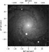 |
Fig. 1. White image obtained combining the light in the full wavelength range of the cropped data cube of the central arc minute. |
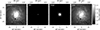 |
Fig. 2. From left to right, kinematic-corrected integrated data cube (given to C2D as an input), and the data cubes of the NSC, the bulge, and the disk. These three components are from the C2D spectrophotometric decomposition. Masked regions are plotted in black. |
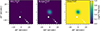 |
Fig. 3. Light ratio of each component over the total light of the galaxy, delivered by C2D. From left to right, NSC fitted as a PSF, bulge, and disk. The NSC dominates the light in the central spaxels within one PSF FWHM. Masked regions are plotted in white. |
Wavelength range cut and Voronoi binning. For the full analysis, we used the wavelength range between 4800 and 5500 Å. Within the MUSE spectral coverage, this range contains the relevant spectral features sensitive to the stellar population parameters of interest, such as Hβ and several Mg and Fe absorption lines indicated in Fig. 4 (e.g., Pinna et al. 2019a,b; Sattler et al. 2023, 2025). At the same time, this range is not as affected as the redder range by sky residuals and imperfections in the modeling of molecular bands of the stellar population models. Using this wavelength range, we applied a Voronoi binning (Cappellari & Copin 2003), using the VORBIN Python package. This method spatially bins the data in an adaptive way, preserving the maximum possible spatial resolution, to reach a target signal-to-noise ratio (S/N) per bin. A mild level of spatial binning was initially needed to reach the required S/N for an acceptable level of accuracy in fitting kinematics, needed for the kinematic correction (see below). We used a target S/N = 25, a good compromise between obtaining reliable velocities and velocity dispersion and preserving a close-to-spaxel resolution, especially in the very central region where our interest resides. Preserving the highest possible spatial resolution is important for the spectro-photometric decomposition, and binning more would have smoothed the spatial information that C2D needs to fit each of the quasi-monochromatic images. We ensured that all included spaxels before binning had a S/N > 3.
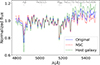 |
Fig. 4. Spectra obtained by integrating, within an aperture of 1σ of the PSF, the prepared kinematic-corrected (original) data cube before the spectrophotometric decomposition (blue solid), the NSC data cube (red dashed), and the host galaxy data cube (green dashed). Some spectral features, relevant for the stellar population analysis, are shown: Hβ, the Mgb triplet (not entirely resolved), and four Fe lines. |
Correction from stellar kinematics. The C2D code performs the spectro-photometric decomposition in each individual quasi-monochromatic image, which is created with the flux in the same spectral pixel, i.e., at the same wavelength position, for all spaxels. When extracting the images, the spectral features in the data cube (e.g., absorption or emission lines) must be located in the same spectral pixels (same wavelength) for all spaxels. Otherwise, one image may mix information from different rest-frame wavelengths. In the observed spectra, spectral features are shifted not only an amount corresponding to the redshift of the galaxy, but also due to (gas- and stellar-) kinematic Doppler effects. Moreover, the observed width of these spectral features is affected by the stellar and gas velocity dispersion. Therefore, before applying C2D, we need all spaxels to have the same velocity (V = 0 km s−1 at the rest frame) and the same line broadening (velocity dispersion). For that, we corrected the data cube from the stellar kinematics of each spaxel. We calculated the LOS velocity and velocity dispersion in each spaxel of our cropped and Voronoi binned data cube, as explained in Sect. 4.2. Accounting for the kinematics in each spaxel, we shifted the entire data cube to the rest frame, and we convolved it to the maximum measured velocity dispersion in the analyzed data cube (∼155 km s−1).
Treatment of the emission lines. Since M 74 is a star-forming galaxy, spaxels in the disk region have emission lines, often strong, in their spectra. We tested C2D on the kinematic corrected data cube both with and without previously subtracting emission lines. The emission cleaning for these tests was conducted using PPXF (Cappellari & Emsellem 2004, see also Sect. 4.2). We finally decided not to feed C2D with the emission-subtracted data cube but instead used the cube including the emission. This choice avoided introducing any additional bias when subtracting emission lines from spectra and gave better C2D fits. Since emission characterizes specific regions, such as the disk-dominated region, but not others, such as the very central NSC-dominated region, preserving these differences helped the C2D code perform a better multicomponent fit. Méndez-Abreu et al. (2019) showed the capability of C2D to process emission lines properly.
4.1.2. Application of C2D to M 74
In this work, we analyze the stellar populations in the NSC of M 74 and compare them with those of the host galaxy. Because the NSC is unresolved, its light was measured within a PSF aperture, while the surrounding galaxy was spatially resolved using the full capabilities of the IFS data. This enabled direct comparison between the NSC and its immediate environment, placing its formation in the context of the host galaxy. We adopted C2D over other spectrophotometric decomposition codes (e.g., BUDDI, Johnston et al. 2017; see also Sect. 1) because it uniquely preserves spectral and spatial information for each component. This allowed us not only to subtract the PSF-weighted NSC light but also to map the host galaxy properties, fully exploiting the spatial information from IFS.
For this work, we adapted C2D and GASP2D to include the following three components: an NSC, a bulge, and a disk. This choice was, on the one hand, motivated by the fact that this galaxy was fitted with a bulge and a disk by Salo et al. (2015) as part of the S4G sample (Sheth et al. 2010). On the other hand, we are mostly interested in the NSC, which is not spatially resolved in MUSE data as its size is smaller than the PSF size (Sect. 3). Its light is spread by the PSF in a larger region than its size, and we follow other studies modeling the NSC as a PSF to disentangle its spectra from the galaxy spectra (e.g., Johnston et al. 2020; Fahrion et al. 2021). We fitted the NSC using the Moffat function from the PSF modeling in Emsellem et al. (2022, see Sect. 2 for more details). While we adopted a FWHM of 0.6 arcsec (three MUSE spaxels), we tested that the results were not affected by variations of ±0.2 arcsec (one spaxel). To test this, we repeated the full decomposition and spectral-fitting process with a FWHM of 0.4 and 0.8 arcsec, finding that the differences in the NSC stellar populations were negligible. The FWHM and the power index (2.8, see Sect. 2) of the Moffat function were fixed in the fitting process, while the PSF (NSC) central intensity was kept free and fitted.
For the bulge and the disk, we used a Sérsic and a broken-exponential two-dimensional profiles, respectively (see Méndez-Abreu et al. 2017 for the specific implementation). We extensively tested different combinations of free and fixed parameters of these profiles, resulting in a better decomposition with a certain number of them fixed, as described below. Furthermore, the impact of small errors in the bulge and disk parameters on the NSC spectra, which is the goal of the decomposition, is negligible. The effective intensity, the effective radius and the Sérsic parameter of the bulge, as well as the central intensity of the disk, were kept free and fitted by the code, while the ellipticity and the position angle of both the bulge and the disk were fixed to the values from the S4G decomposition by Salo et al. (2015), who fitted the disk with a single exponential. We checked that the effective radius and the Sérsic parameter of the bulge resulting from the fit were very similar to the values from Salo et al. (2015). We did not expect to find the same values since they used a different wavelength range compared to ours.
Before choosing a broken exponential for the disk profile, we performed a preliminary morphological analysis, fitting ellipses to the isophotes, in an image obtained from the entire PHANGS-MUSE mosaic, integrating all wavelengths in the analyzed spectral range. A one-dimensional radial profile, obtained by averaging azimuthally, follows a broken exponential, with the outer-profile scale length matching the disk scale length from S4G (Salo et al. 2015, using a single exponential). This is in agreement with the fact that the S4G team performed the morphological fit on a much larger spatial scale. We measured that the inner exponential has a scale length of 17.4 arcsec (∼827 pc) while the break radius is located at 30 arcsec (∼1.4 kpc) from the center. While our cropped data cube is dominated by the inner exponential, we fixed both of these parameters in the C2D decomposition. With our new setup, GASP2D fitted each quasi-monochromatic image with a combination of a bulge, a disk and a NSC. This resulted in three data cubes, one for each component. Images resulting from integrating all wavelengths for each data cube are shown in Fig. 2. The light fractions of each component over the total are shown in two dimensions in Fig. 3. This figure shows that the NSC dominates the light (with a light fraction above 60%) in the central spaxels within one PSF FWHM, while 100% of the light was assigned to the disk from a certain radius (∼7 arcsec) outward.
Since we are interested in the stellar population properties of the NSC and its comparison with the surrounding host galaxy, for the rest of the analysis we use a data cube for the NSC and another for the rest of the galaxy. The latter was obtained by combining the bulge and the disk data cubes, and it corresponds to the host galaxy, i.e., the galaxy after subtracting the NSC. We preferred this approach instead of considering the bulge and the disk separately to minimize the impact of a potential suboptimal decomposition of these two morphological structures. This also follows previous studies of this kind, comparing the NSC to the host galaxy as a whole (Johnston et al. 2020; Fahrion et al. 2021). However, the C2D approach, providing spatially resolved spectral information, additionally allowed us to fairly compare NSC properties with the host galaxy in the same aperture. This minimized biases derived from quantitative comparisons of different spatial regions due to spatial gradients in the host galaxy.
We extracted integrated spectra in an aperture of radius 1σ of the PSF FWHM (∼0.26 arcsec ≈12 pc) from these two data cubes and, for comparison, from the “original” kinematic-corrected data cube before being processed by C2D (Sect. 4.1.1). Taking into account the central region of the PSF ensures that small errors in its estimate and variations of its size with wavelength have no impact on the extracted properties of the NSC. Hereafter, we refer to (1) the NSC spectrum and data cube as the one corresponding to the NSC component as extracted by C2D, (2) the “host galaxy” spectra and data cube as the one obtained combining the C2D disk and the bulge (and corresponding to the galaxy after subtracting the NSC), and (3) the “original” spectrum and data cube as the original one before the C2D decomposition and containing the three morphological components (i.e., the full galaxy). These spectra are shown and compared to each other, for 1σ PSF, in Fig. 4.
4.2. Spectral fitting
We used a full-spectrum fitting technique both for the stellar population analysis (of all previously mentioned integrated spectra and data cubes), and for the calculation of the kinematic parameters necessary for their correction, as explained in Sect. 4.1.1. We used the latest Python implementation of the penalized pixel-fitting (PPXF) method (Cappellari & Emsellem 2004; Cappellari 2017, 2023). PPXF models an observed spectrum as a linear combination of simple stellar population (SSP) templates, convolved with a line-of-sight velocity distribution (LOSVD) described by a Gauss–Hermite series. The resulting (light- or mass-fraction) weights, assigned to the SSP models to obtain the best-fit spectrum, can be used for the stellar population analysis, while the line-of-sight velocity distribution can be used to extract the kinematic parameters. In this work, different PPXF setups were used to extract stellar populations and kinematics. Stellar velocities and velocity dispersions were derived by fitting the central data cube resulting from the preparation described in Sect. 4.1.1, with PPXF, using an additive polynomial of degree 8, and no multiplicative polynomial. Additive polynomials are typically used to minimize the effect of template mismatch in the kinematic fitting (Cappellari & Emsellem 2004; Cappellari 2017).
The stellar population analysis was carried out applying PPXF to the NSC and host galaxy data cubes and PSF-integrated spectra, resulting from the C2D decomposition (Sect. 4.1.2). For comparison, the “original” data cube (before the C2D decomposition, but kinematic corrected) was also analyzed in the same way. The PPXF setup used for the stellar populations included a multiplicative polynomial of 8th order. Multiplicative polynomials are typically used to minimize the effect of imperfections in the flux calibration and dust reddening (Cappellari & Emsellem 2004; Cappellari 2017). On the other hand, additive polynomials are typically avoided in the calculation of ages and metallicities as they could affect absorption line strengths and bias the results (e.g., Guérou et al. 2016). While the emission lines are strong in most disk-dominated regions of this star-forming galaxy, there is no clear emission in the very central region (Fig. 4). The Hβ absorption line is an essential age indicator in the MUSE wavelength range (e.g., Worthey 1994), and we decided not to mask it in the analysis of the PSF size of the data cubes (results in Sect. 5.1). However, we needed to mask Hβ in the analysis of the host galaxy data cube (results in Sect. 5.3), since in the disk-dominated region the emission is strong. In all cases, we masked the other typical emission lines in the analyzed wavelength range ([O III]λλ4959,5007 and [N I]λλ5198,5200).
We used in this work the semi-empirical sMILES SSP models (Knowles et al. 2023), the most up-to-date version of the MILES SSP models (Vazdekis et al. 2010, 2015). sMILES models are based on BaSTI isochrones (Pietrinferni et al. 2004, 2006) and offer five different values of the [Mg/Fe] abundances, covering the range between −0.2 and 0.6 dex (in steps of 0.2 dex). Throughout this paper, we use [Mg/Fe] as a proxy for the enhancement in α elements. sMILES models cover ages between 0.03 and 14 Gyr, with 53 different values, and ten values of total metallicities [M/H] between −1.79 and 0.26 dex. This gives a total of 2650 SSP models. Since each of them corresponds to one combination of age, [M/H] and [Mg/Fe], coupling these models with PPXF allowed us to extract the distribution of these three stellar population parameters from each spectrum (given by the distribution of weights given to the different SSPs). These models cover a wavelength range between 3540 and 7409.6 Å, at a spectral resolution of 2.51 Å at FWHM. Among sMILES sets of models, we chose the set of SSPs that adopted a bimodal initial mass function with a logarithmic slope of 1.3 for the segment of massive stars (Vazdekis et al. 2003). These models were normalized to correspond to one solar mass each, so that mass-weighted results are obtained from PPXF if SSPs are not renormalized. They need to be renormalized to their own median to obtain light-weighted results. In this work, we used light-weighted results to obtain the stellar population maps and mass-weighted results to reconstruct SFHs in terms of mass fractions corresponding to different stellar populations.
Our general approach for the stellar population analysis was to average results from Monte Carlo simulations of unregularized PPXF fits, following Cappellari (2023). We used this approach to fit the three spectra extracted from the PSF aperture (Sect. 4.1.2), i.e., the NSC, the host galaxy, and for comparison the spectrum from the original integrated data cube. We performed 100 Monte Carlo realizations for each spectrum. For each realization, we perturbed the spectrum with random, wavelength-dependent noise drawn from a Gaussian distribution. The noise level was taken from the residuals at the specific wavelength, from an initial (unregularized) PPXF fit. From the distribution of SSP weights for the 100 realizations, we estimated the mean ages, [M/H] and [Mg/Fe], and their statistical uncertainties (as standard deviations), for each of the three spectra. This allowed us not to use any regularization on the SSP weights during the PPXF fits.
The resulting host galaxy data cube from the decomposition was rebinned to a higher S/N of 100 before performing the spectral fitting for the spatially resolved stellar population analysis, ensuring robust results and lower uncertainties in the outer, fainter region. This still left us with 6766 Voronoi bins, which made the Monte Carlo approach time-consuming and computationally expensive for the entire data cube. Thus, we decided to map the stellar population parameters of the host galaxy using PPXF regularized fits with a unit regularization parameter. While one single unregularized fit gives discrete and noisy solutions, some level of regularization ensures smoother and more realistic stellar population solutions (e.g., Cappellari 2017). However, regularization above a certain level can lead to biases in the results and dilute features in the SFHs. Thus, we used the approach presented in Pinna et al. (2019b) to choose the regularization parameter (described as follows, see also Pinna et al. 2019a; Martig et al. 2021; Sattler et al. 2023, 2025). After rescaling the PPXF noise parameter as the one necessary to obtain a reduced χ2 = 1 with no regularization, we choose a regularization well below a certain maximum calibration value. We defined the calibration regularization as the minimum value increasing χ2, from the case with no regularization, by 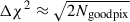 , where Ngoodpix is the number of fitted (spectral) pixels (McDermid et al. 2015; Cappellari 2017; Boecker et al. 2020). This approach was also used to map the stellar populations from the original data cube before the C2D decomposition (Appendix A).
5. Results
5.1. Stellar populations within a central PSF aperture: Average properties and SFHs of the NSC compared with the host galaxy
We present here the average stellar population properties and SFHs, both reconstructed from the weights given to the SSP models by the spectral-fitting approach detailed in Sect. 4.2. All these results were extracted from the three spectra integrated within an aperture of 1σ PSF (Sect. 4.1.2) and shown in Fig. 4.
We present in Table 1 the average light- and mass-weighted stellar population properties of the NSC and the host galaxy and their uncertainties, calculated as a weighted average using the light or mass weights from the spectral fitting. For reference, we also present the results from the original integrated data cube, before the C2D decomposition. While we show in Table 1 both light- and mass-weighted results, differences between different components are enhanced in the light-weighted results, which in general give more weight to younger stars. The NSC is very old, with an average light-weighted age of ∼11 Gyr. It is metal poor ([M/H]LW ∼ −0.6 dex) and slightly enhanced in α elements with respect to the Sun ([Mg/Fe]LW ∼ 0.1 dex). The host galaxy, in the central 1σ PSF aperture, shows much younger (light-weighted) ages (∼5 Gyr), higher and supersolar metallicities ([M/H]LW ∼ 0.2 dex) and about solar (light-weighted) [Mg/Fe] abundances. These results reveal that the NSC is much older and more metal poor than its host galaxy, suggesting that it was formed a long time ago, when the interstellar medium was not chemically enriched yet, and was not involved in the later active star formation of the host galaxy. [Mg/Fe] is only slightly more enhanced in the NSC than in the center of the host galaxy. Since the α enhancement is usually interpreted as a formation in a faster time scale (e.g., Matteucci 1994), this suggests that the formation time scale of the NSC may have been slightly faster than the central region of the host galaxy. This is in agreement with NSC’s old age and low metallicity, suggesting that NSC formation was relatively short in time.
Average stellar population properties and their uncertainties.
On the other hand, the difference between the mass-weighted ages of the NSC and its host galaxy is smaller (than when considering light-weighted ages), with the stars in the host galaxy being only about 2 Gyr younger than the NSC. The smaller age difference between the host galaxy and the NSC, in the mass-weighted averages, stems from an older host galaxy age. This suggests that, while the disk light is dominated by young stars, it also contains a significant (mass) fraction of old populations. However, this is still a significant difference for mass-weighted results, which are expected to be generally biased toward older ages (e.g., Sánchez-Blázquez et al. 2014b; Sattler et al. 2023, 2025). Mass-weighted and light-weighted metallicities are quite similar to each other, while light-weighted [Mg/Fe] abundances are slightly higher than the mass-weighted ones. Uncertainties indicated in Table 1 were obtained via Monte Carlo simulations (Sect. 4.2). Differences in the stellar population properties of the different components are larger than these uncertainties, and thus they can be considered significant. However, these represent only statistical uncertainties, and they are relatively low for such high S/N spectra. Systematic uncertainties, such as those due to imperfections in the SSP models, are very challenging to estimate and are not taken into account here.
From the mass weights obtained in the full spectral fitting process, we also reconstructed the SFHs in terms of the stellar mass assigned to different age bins. Compared to the average properties presented above, SFHs were obtained by averaging only the mass weights given to coeval SSPs. We show these SFHs in Fig. 5 in the top and middle panels. In the bottom panel, we show, as a reference, the SFH of the full non-decomposed galaxy, extracted from the same PSF aperture in the kinematic-corrected original MUSE data cube before the C2D decomposition (blue spectrum in Fig. 4). The NSC shows distinct stellar populations at old ages, with the highest mass fractions distributed in ages between 10 and 11 Gyr. The host galaxy shows an old component made of two peaks of different ages (∼10 and ∼12 Gyr) and a relatively recent component with ages of about 2 Gyr and younger. Some intermediate-age populations are also present (∼6 Gyr). The SFH of the full galaxy (bottom panel) shows a combination of all these components. A word of caution is deserved by the large uncertainties, indicated by the shades in each panel of Fig. 5. These shades cover the region between the 16% and 84% percentiles, calculated on the distribution of the 100 Monte Carlo realizations. Since mass fractions are normalized to the total mass in each SFH (in each fitted spectrum), these errors indicate that some mass fraction assigned to the highest peaks could be, in reality, redistributed to minor peaks. Overall, the SFHs suggest that the center of the galaxy had an intense early phase of star formation, between 14 and 8 Gyr ago, when the NSC stars formed. Afterward, it experienced a long quiescent phase, with a very low star formation rate. Only relatively recently (later than 3 Gyr ago), a more active star formation was reactivated in M 74. However, while this episode involved an extended region of the disk and was enhanced in spiral arms, as shown in Fig. 6, it did not affect the NSC, as this remained old and metal poor. Sánchez-Blázquez et al. (2014a) found a very similar SFH for M 74, using the STEllar Content via Maximum A Posteriori likelihood (STECKMAP) spectral-fitting code (Ocvirk et al. 2006).
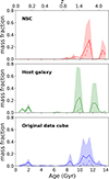 |
Fig. 5. Star formation histories of the NSC, the center of the host galaxy, and both components together (from the “original” MUSE data cube), from top to bottom. The three panels were plotted using the mass-weighted results from fitting spectra integrated in a central PSF aperture (Sect. 4.1.2 and Fig. 4). Mass fractions have been normalized to the mass of each component within the PSF aperture. The solid lines indicate the mean mass fraction for each age bin (half a billion year wide), calculated on the weight distributions from the 100 Monte Carlo realizations (Sect. 4.2). Dashed lines follow the median, and shades indicate the 16th and 84th percentiles from the distributions. |
 |
Fig. 6. Stellar population maps of the host galaxy component of M 74 after subtracting the NSC. From top to bottom, light-weighted age, total metallicity [M/H], and [Mg/Fe] abundance. The masked regions are depicted in white and isophotal contours in black. The physical scale is given as a reference in the top axis. |
5.2. Additional tests and comparisons
We first compared the results above with the stellar populations obtained from a central PSF aperture in the kinematic-corrected original data cube (spectrum indicated as a blue solid line in Fig. 4). This contains the integrated light of the NSC and the host galaxy together and, as expected, gives intermediate stellar populations between the NSC and the host galaxy (Table 1). We also compared the stellar populations in a central PSF aperture with the surrounding region of the galaxy, both extracted from the original data cube. To do so, we calculated the average ages, [M/H] and [Mg/Fe] within a much larger central aperture of 100 pc (excluding the central 3σ PSF to make sure the contamination from the NSC is negligible). For this, we used the stellar population maps extracted from the original integrated data cube (Appendix A). These stars are younger (5.6 Gyr) and slightly more metal rich (−0.1 dex), than the stars in the central PSF aperture extracted from the same original data cube (Table 1). However, the [Mg/Fe] abundance is very similar (0.1 dex). The fact that the original data cube, including the light of stars of both the NSC and the host galaxy, shows gradients with older and more metal-poor stars in the very center, is in perfect agreement with the presence of an older and more metal-poor component in the center (i.e., the NSC), which is not present in the surroundings.
We also tested the robustness of this gradient by fitting a spectrum from the original data cube but integrated now in a 3σ PSF (about 40 pc, with a much stronger contribution from the host galaxy). In a 3σ PSF aperture, we find ages about 1 Gyr younger than integrating within a 3σ PSF, in the original and host galaxy data cubes, while the NSC age remains the same. Since we were comparing results from slightly different methods (on the one hand, fitting spectra integrated in specific apertures, on the other hand, averaging stellar population properties in the spatially resolved maps shown in Appendix A), we checked that the same results were found within 1σ PSF with the different methods. The mean age, [M/H], and [Mg/Fe] from a 1σ PSF aperture in the spatially resolved maps in Fig. A.1 are respectively 6.8 Gyr, −0.2, and 0.1 dex, thus approximately the same as the results from fitting a spectrum from the original data cube obtained integrating in a 1σ PSF aperture (shown in Table 1).
To additionally test how robust our C2D method is, we also compared our results with the ones from an NSC spectrum obtained by subtracting the underlying host galaxy light from a PSF integrated spectrum (‘original’, in Fig. 4). Following Fahrion et al. (2021), the host galaxy spectrum was obtained from an annulus surrounding the NSC, with inner and outer radii of 0.8 (∼3σ PSF) and 2 arcsec. Before subtracting the host galaxy spectrum from the “original” spectrum, the annulus spectrum needs to be first rescaled to the light of the host galaxy in the same central PSF aperture where the “original” spectrum was integrated (brighter than the annulus). While Fahrion et al. (2021) performed a dedicated morphological decomposition to calculate the scaling factor, we used our decomposition from C2D. We obtained again very old light-weighted ages (8.5 ± 1.1 Gyr), low metallicities (−0.39 ± 0.04 dex) and close to solar [Mg/Fe] enhancement (0.01 ± 0.03 dex). While these results give small differences (taking into account the uncertainties – slightly younger ages and higher metallicities), they are closer to the results from C2D than what was obtained from the original data cube. While it is not surprising that different methods give slightly different results (see also Sect. 6.1), our method is more sophisticated than simply subtracting spectra. Our method leads to a cleaner NSC spectrum than the simple subtraction and therefore to larger differences between results from integrated and decomposed spectra. The main reason for this is that C2D performs a fitting spaxel by spaxel and spectral pixel by spectral pixel, while when subtracting the annulus spectrum from the PSF spectrum we are forced to take an “average” spectrum within the annulus, and the scaling factor is also calculated using integrated light. More importantly, these differences are not critical for the interpretation of our results: the NSC appears to be very old and metal poor, and much older and more metal poor than the host galaxy according to the results obtained with all methods.
5.3. Spatially resolved stellar populations of the host galaxy
Spatially resolved properties of the host galaxy are important to interpreting the NSC properties in the context of its surroundings. We mapped the mean age, [M/H] and [Mg/Fe] of the host galaxy, fitting the host galaxy data cube decomposed with C2D (Sects. 4.1.2 and 4.2). The maps are shown in Fig. 6. Both [M/H] and [Mg/Fe] are presented in logarithmic scale and with respect to solar values (zero values correspond to solar values). The age map (top panel) shows a relatively young host galaxy (with most regions younger than ∼4 Gyr). A pattern following the spiral arms can be identified, with alternative regions dominated either by young (about ∼2 Gyr-old or younger) or old stars (older than ∼8 Gyr). The [M/H] map (middle panel) displays a clear negative radial gradient, with a central metal-rich region of about 500 pc size (supersolar metallicities). Outer regions have higher and lower values alternatively. [Mg/Fe] abundances are mostly anti-correlated with [M/H], showing the lowest values (close to solar) in the central metal-rich ∼500 pc. Hints of the spiral-arm shape are visible in both [M/H] and [Mg/Fe] maps, whose values do not necessarily follow any correlation or anti-correlation with age. However, the youngest (outer) regions in the analyzed data cube show a strong α enhancement in some metal-poor blobs.
Masking Hβ might introduce an age bias in the map of the host galaxy, with respect to the analysis of the central PSF size, in which we directly fitted Hβ since there was no visible emission (see Sect. 4.2 for details). However, we verified that fits of the host galaxy PSF-sized spectrum give similar results, no matter whether Hβ is masked or not. Thus, we can qualitatively compare the results in Sect. 5.1 with the maps shown here. The NSC is as old as some outer interarm disk-dominated regions in the host galaxy age map in Fig. 6, while the rest of the host galaxy is much younger. The old metal-poor NSC resides in the relatively young and very metal-rich central ∼500 pc of the host galaxy.
However, the NSC is as metal poor as some young regions of the disk. Regarding [Mg/Fe], the NSC has a similar abundance to its surrounding galaxy. These results suggest that while M 74 kept forming stars in most of its disk, this did not happen in some specific regions. While more recent star formation occurred in the central region of the galaxy, allowing for an extended chemical enrichment, this did not happen in the NSC, which remained old and metal poor.
In Appendix A, we present for reference the analysis of the original MUSE data cube before the spectro-photometric decomposition. Although the Voronoi binning is slightly different, Fig. A.1 shows similar trends to Fig. 6. The difference between the original data cube and the host galaxy decomposed data cube is that the former includes the light of the NSC, which was extracted from the latter. Thus, we can expect a difference in the stellar populations only in the region where the NSC dominates. Indeed, as described in Appendix A, a clear [M/H] drop is visible within a PSF size in Fig. A.1. Our results for the central region of M 74 are in agreement with the stellar population analysis by Pessa et al. (2023, see also Sect. 3).
6. Discussion
6.1. The nuclear star cluster in M 74 and its formation
We found old ages (∼11 Gyr), low metallicities ([M/H] ∼ −0.55), and no particular α enhancement ([Mg/Fe] ∼ 0.1) in the NSC hosted by the relatively massive spiral galaxy M 74. We found older ages and lower metallicities in the NSC compared to results from Hoyer et al. (2023b, 8 ± 3 Gyr and Z = 0.012 ± 0.006, corresponding to [M/H] ∼ −0.2 dex). However, our results for the decomposed NSC are compatible within their large uncertainties. They used a different method and wavelength range (spectral energy distribution fitting of HST and JWST photometry; see also Sect. 3). They did not decompose the light of the NSC from the host galaxy in the LOS, but they could spatially resolve the NSC. These reasons can explain the differences, as they found ages and metallicity values more similar to our results before the spectro-photometric decomposition (from the “Original” spectrum, in Table 1).
Our stellar population analysis has shown an ancient and metal-poor NSC, surrounded by a much younger and more metal rich region of the host galaxy. As shown by JWST observations (Hoyer et al. 2023b), the NSC lives in a cavity with no gas or dust, while being hosted by an actively star-forming galaxy with a complex structure of gas and dust filaments. The cavity formed due to some processes either keeping gas and dust out of it or wiping them out of the central region (see also Sect. 6.3). While the presence of a massive black hole in M 74 is still under debate, the presence of a low-luminosity AGN has been proposed by different authors (e.g., Dong & De Robertis 2006; She et al. 2017). It is also one of the possible explanations for the presence of the cavity (all gas may have been blown away via AGN feedback, which is all the more likely if the black hole activity was much stronger in the past) and of the mid-infrared emission found at the center of the galaxy with JWST observations (Hoyer et al. 2023b). Similarly, central quiescent regions (of about 100 pc sizes), surrounded by starbursts, as well as nuclear older ages (within radii from a few parsecs to ∼50 pc) than the circumnuclear regions, were previously detected in AGN hosts (e.g., Márquez et al. 2025; da Silva et al. 2025). Other, more unlikely explanations for the fact that no gas in an amount sufficient to trigger star formation reached the NSC in the last ∼8 Gyr, could be a previous overall scarcity of gas in the galaxy (not happening now since the galaxy is overall gas rich), and the lack of a clear and strong bar structure, which would help gas inflow, combined with dynamical processes making gas inflow inefficient.
In any case, the presence of the cavity may have affected the evolution of the NSC, which could not grow via in situ star formation due to the lack of gas. However, the surrounding region of the NSC, including stars in the region of the cavity, is much younger and more metal rich. Our decomposition, supported by the analysis of spectra in the original data cube integrated into different apertures (Sect. 5.2), suggests that these younger stars belong to the galaxy disk. The middle panel in Fig. 5 suggests that the center of the host galaxy had later and relatively recent episodes of star formation. This did not happen in the NSC, whose stars were all formed at the early stages of the evolution of M 74. Its SFH shows that its stars were all formed more than 8 Gyr ago. Regarding the origin of these old and metal-poor stars, we cannot say if they were formed in situ a long time ago, when the gas in M 74 was still metal poor. Old ages and low metallicities (although typically lower than what we find here) in NSCs are traditionally explained by globular cluster inspiral (Neumayer et al. 2020; Fahrion et al. 2021, 2022b,a). While globular cluster migration is thought to be the dominant formation mechanism for NSCs less massive than the one in M 74 and hosted by low-mass galaxies, our results do not provide enough information to rule out (or support) this scenario versus a very early in situ formation (see also Sect. 6.3). Furthermore, the presence of LMXBs in the NSC suggested by the nuclear X-ray emission (see Sect. 3), consistent with the NSC old age, provides additional support for the NSC to be one or more globular clusters that migrated to the galactic center.
6.2. M 74 might have a nuclear star cluster that is unique for its type and mass
The NSC in M 74 shows common stellar population properties with other NSCs in the literature. However, it is important to discuss NSC properties in the context of their host galaxies. Fahrion et al. (2021) analyzed NSCs in a sample of 25 ETGs in the Fornax and Virgo clusters, finding several of them as old as the NSC in M 74 and very metal poor. However, while the sample includes galaxies of similar stellar masses to M 74 (Sect. 3), the NSCs with the most similar stellar populations to the one in M 74 were lower-mass NSCs (≲106 M⊙) hosted by less massive, mostly quiescent ETGs (≲109 M⊙). ETGs of similar masses as M 74 host metal-rich NSCs. Among the seven dwarf ETGs in the Fornax cluster, analyzed by Johnston et al. (2020), NSCs with similar ages to the one in M 74 are much more metal poor. These NSCs and their dwarf host galaxies are systematically more metal poor than in the M 74 case. NSC age in M 74 is also similar to that of three NSCs from Fahrion et al. (2022a), who analyzed a sample of nine star-forming dwarf LTGs. While these galaxies are star-forming and have morphological types more similar to M 74, they have much lower stellar masses (∼107 to ∼109 M⊙). These host galaxies and their NSCs also show systematically lower metallicities than M 74 and its NSC. Some NSCs hosted by galaxies more similar to M 74 in terms of morphological types and masses were analyzed by Kacharov et al. (2018). However, while some have similar metallicities to M 74’s NSC (see also Walcher et al. 2006), they are all relatively young. While there are other spiral galaxies with NSC ages similar to the one in M 74, these galaxies are slightly earlier types than M 74 (Rossa et al. 2006).
While previous studies in the literature show other NSCs with similar stellar population properties, suggesting that the NSC of M 74 is not unique, no NSCs hosted by a relatively young, metal-rich, massive star-forming (late-type) spiral galaxy, have been reported to have such old ages. This suggests that the properties of M 74’s NSC are not common in its host galaxy context, and this NSC may have had a peculiar formation and evolution history. It is quite extraordinary that in such a gas-rich spiral galaxy, no significant amount of gas triggered any in situ star formation in the NSC over the last ∼8 Gyr. The inefficiency of gas inflow to the nucleus in this gas-rich star-forming galaxy is what makes M 74 unusual, resulting in its ancient NSC.
6.3. Nuclear star cluster formation and the host galaxy evolution
Different NSC properties have been found in galaxies of different masses (Sect. 1). This was explained with a transition in the dominant mechanisms driving NSC formation and growth, with in situ star formation being dominant in higher mass galaxies, and globular cluster migration to the center of a galaxy dominating at lower masses (e.g., Fahrion et al. 2021, 2022b,a). Among others, one piece of evidence is the transition in the NSC metallicity regime at galaxy stellar masses of about 109 M⊙ (e.g., Neumayer et al. 2020). In more massive galaxies, NSCs tend to be more metal rich, with [Fe/H] metallicities about ±0.5 dex around solar. For lower galaxy masses, on the other hand, NSCs have metallicities in a wide range, including very low values. In Fig. 7, we have reconstructed this trend as shown in Fig. 9 of Neumayer et al. (2020), and updated it with additional measurements (NSCs from Fahrion et al. 2021, 2022a; Kacharov et al. 2018). NSCs in LTGs are shown in blue, and show, on average, lower metallicities than NSCs in ETGs (red symbols). Note also that blue triangles are total metallicities ([M/H], from Fahrion et al. 2022a), and they have to be considered upper limits for [Fe/H] metallicities. While more points will be needed to shed more light on this trend, the available points suggest that the trend of more metal-rich NSCs being hosted by more massive galaxies, clearly shown for ETGs, also holds for LTGs (but with a lower average metallicity). For higher-mass spirals, we only have four NSCs from the literature (Kacharov et al. 2018, blue circles), which appear to display lower metallicities than, on average, NSCs in ETGs of similar masses.
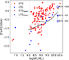 |
Fig. 7. Metallicity of the NSC as a function of the galaxy stellar mass (figure reconstructed and updated from Fig. 9 in Neumayer et al. 2020). The blue open circle indicates the [Fe/H] metallicity of the decomposed NSC of M 74. For comparison, [Fe/H] of the decomposed host galaxy is indicated with an open square, while a star indicates the [Fe/H] from the original (integrated) data cube of M 74 (see the text for all the details). The ETGs are indicated in red and LTGs in blue. Red circles are points from spectroscopic and photometric data (Koleva et al. 2009; Paudel et al. 2011; Spengler et al. 2017; Kacharov et al. 2018), as from Neumayer et al. (2020). The two solid black lines are the mass-metallicity relations of galaxies, given as reference, at the low-mass end (Kirby et al. 2013) and the high-mass end (Gallazzi et al. 2005). We have added the red triangles, which are NSC total metallicities ([M/H]) from Fahrion et al. (2021) and are therefore considered as upper limits for [Fe/H]. We have also added all the blue points. Blue triangles are for [M/H] and are thus upper limits of the NSCs in dwarf LTGs in Fahrion et al. (2022a). Blue circles are for the NSC [Fe/H] in more massive LTGs in Kacharov et al. (2018). |
For M 74, [Fe/H] was calculated from [M/H] and [Mg/Fe] in Table 1 following the relation [Fe/H] = [M/H] − 0.75[Mg/Fe] from Vazdekis et al. (2015). M 74’s NSC (blue open circle), is more metal poor than the rest of NSCs in Fig. 7 for similar galaxy masses, even if compared with the few LTGs. M 74 is located, in Fig. 7, in a mass regime where NSCs are thought to be dominated by in situ formation, as suggested by their usually higher metallicities than their host galaxies (Fahrion et al. 2022b). However, its host galaxy (blue open square) is much more metal rich than the NSC (about 0.7 dex difference in [M/H] within the central PSF region). In general, NSC old ages and low metallicities, in particular if older and more metal poor than the host galaxy, have been interpreted as a main formation through globular cluster inspiral (e.g., Fahrion et al. 2021). If compared with other star clusters in M 74, its NSC shows similar ages to the most massive globular clusters (Whitmore et al. 2023), supporting the cluster migration scenario. On the other hand, models predict that NSCs of the mass of the one in M 74 (∼107 M⊙) assembled slightly more than half of their mass via in situ star formation and the rest through globular cluster inspiral (Fahrion et al. 2022b). Recent JWST studies at high redshift have recently proposed that similar very dense objects existed already in the early universe and may have been the first structure that a galaxy formed (e.g., Bellovary 2025; Graham et al. 2025). These high-redshift objects may have much in common with NSCs, ultra-compact dwarfs and stripped nuclei in the local universe. The old, metal-poor NSC in M 74, with very different stellar populations from the host galaxy, may have formed either by the later migration and merging of star clusters whose stars formed at very early stages or by very early in situ formation. Several cluster accretion episodes, different bursts of in situ star formation, or a combination of both might have led to the different peaks in the SFH in Fig. 5.
7. Conclusions
We have analyzed the stellar populations of the NSC in M 74 and compared it with the host galaxy. We used a spectro-photometric decomposition method, C2D, to separate the NSC light from the host galaxy. This method applies a morphological decomposition for different wavelengths, preserving variations both in the spatial and spectral directions. We performed a separate analysis, in a PSF aperture, of the NSC and the host galaxy, which allowed us to compare them. Additionally, we mapped the spatially resolved stellar population properties of the central ∼3 kpc of the host galaxy. We have reported the light- and mass-weighted ages, the metallicities and [Mg/Fe] abundances, and reconstructed SFHs.
We found an NSC average age of about 11 Gyr and a total metallicity [M/H] of about −0.5 dex. The SFH of the NSC shows that it is exclusively made up of old stellar populations. These results indicate that NSC stars formed during the earliest stages of the evolution of M 74, probably spanning two to three distinct episodes. While we cannot track the potential migration of these stars from other regions of the galaxy and we did not find hints of their accretion from galaxy satellites, our results do not show later contributions from stars younger than ∼8 Gyr. The NSC appears to have remained inactive for a long time in terms of star formation and chemical evolution. Interestingly, this NSC lives in a cavity (with a size of ∼300 pc) devoid of gas and dust, while the rest of the galaxy shows a complex web of gas and dust filaments, where star formation is currently happening. Stellar population maps of the host galaxy have shown young ages in the spiral arms and a very metal rich ∼500 pc central region, with lower [Mg/Fe] values close to solar values. This indicates that the surroundings of the NSC kept evolving over time, while its evolution stopped. A comparison of spectra extracted with a central PSF aperture for the NSC and the host galaxy showed that in contrast to the short NSC evolution, the center of the host galaxy had relatively recent star formation episodes, in addition to the old populations coeval with the NSC.
Finally, the NSC in M 74 is much more metal poor than not only its host galaxy but also other NSCs hosted by ETGs of the same mass as M 74. While there are no measurements for spiral galaxies of the same mass as M 74, its NSC is more metal poor than other NSCs in slightly lower-mass LTGs, with stellar masses between 109.5 and 1010 M⊙. The literature measurements mentioned above might be contaminated by the light of the host galaxy. Our spectro-photometric decomposition method allowed us to obtain a cleaner view of the stellar populations of the NSC otherwise contaminated by the host galaxy (as shown in Table 1 by the analysis of the “Original” data cube). While these findings would traditionally be interpreted as a dominant NSC formation through globular cluster migration and merger at the center of the galaxy, they also suggest that low metallicities might emerge from in situ star formation (at early times) in massive LTGs. With the analysis of a larger sample of massive spiral galaxies, we can find out whether the NSC in M 74 is a unique case or if its stellar populations are common in star-forming galaxies of similar masses, providing additional insights on NSC formation.
Acknowledgments
FP acknowledges support from the Horizon Europe research and innovation programme under the Maria Skłodowska-Curie grant “TraNSLate” No 101108180, and from the Agencia Estatal de Investigación del Ministerio de Ciencia e Innovación (MCIN/AEI/10.13039/501100011033) under grant (PID2021-128131NB-I00) and the European Regional Development Fund (ERDF) “A way of making Europe”. FP wishes to acknowledge the contribution of the IAC High-Performance Computing support team and hardware facilities to the results of this research. MB acknowledges support by the ANID BASAL project FB210003. This work was supported by the French government through the France 2030 investment plan managed by the National Research Agency (ANR), as part of the Initiative of Excellence of Université Côte d’Azur under reference No. ANR-15-IDEX-01. This research was funded, in whole or in part, by the French National Research Agency (ANR), grant ANR-24-CE92-0044 (project STARCLUSTERS). We thank the German Science Foundation DFG for financial support in the project STARCLUSTERS (funding ID KL 1358/22-1 and SCHI 536/13-1). MQ acknowledges support from the Spanish grant PID2022-138560NB-I00, funded by MCIN/AEI/10.13039/501100011033/FEDER, EU. KG is supported by the Australian Research Council through the Discovery Early Career Researcher Award (DECRA) Fellowship (project number DE220100766) funded by the Australian Government.
References
- Agertz, O., Pontzen, A., Read, J. I., et al. 2020, MNRAS, 491, 1656 [Google Scholar]
- Arca Sedda, M., Gualandris, A., Do, T., et al. 2020, ApJ, 901, L29 [Google Scholar]
- Arca-Sedda, M., & Capuzzo-Dolcetta, R. 2014, MNRAS, 444, 3738 [NASA ADS] [CrossRef] [Google Scholar]
- Ashok, A., Seth, A., Erwin, P., et al. 2023, ApJ, 958, 100 [NASA ADS] [CrossRef] [Google Scholar]
- Bacon, R., Accardo, M., Adjali, L., et al. 2010, SPIE Conf. Ser., 7735, 773508 [Google Scholar]
- Bacon, R., Vernet, J., Borisova, E., et al. 2014, The Messenger, 157, 13 [NASA ADS] [Google Scholar]
- Barnes, A. T., Watkins, E. J., Meidt, S. E., et al. 2023, ApJ, 944, L22 [NASA ADS] [CrossRef] [Google Scholar]
- Bekki, K. 2007, PASA, 24, 77 [Google Scholar]
- Bekki, K., Couch, W. J., & Shioya, Y. 2006, ApJ, 642, L133 [Google Scholar]
- Bellovary, J. 2025, ApJ, 984, L55 [Google Scholar]
- Boecker, A., Leaman, R., van de Ven, G., et al. 2020, MNRAS, 491, 823 [Google Scholar]
- Böker, T., Laine, S., van der Marel, R. P., et al. 2002, AJ, 123, 1389 [Google Scholar]
- Böker, T., Sarzi, M., McLaughlin, D. E., et al. 2004, AJ, 127, 105 [CrossRef] [Google Scholar]
- Brown, G., Gnedin, O. Y., & Li, H. 2018, ApJ, 864, 94 [NASA ADS] [CrossRef] [Google Scholar]
- Buta, R. J., Sheth, K., Athanassoula, E., et al. 2015, ApJS, 217, 32 [Google Scholar]
- Cappellari, M. 2017, MNRAS, 466, 798 [Google Scholar]
- Cappellari, M. 2023, MNRAS, 526, 3273 [NASA ADS] [CrossRef] [Google Scholar]
- Cappellari, M., & Copin, Y. 2003, MNRAS, 342, 345 [Google Scholar]
- Cappellari, M., & Emsellem, E. 2004, PASP, 116, 138 [Google Scholar]
- Capuzzo-Dolcetta, R. 1993, ApJ, 415, 616 [NASA ADS] [CrossRef] [Google Scholar]
- Ck, A., Mayya, D., Bressan, A., & Alzate Trujillo, J. A. 2025, ApJ, 984, 21 [Google Scholar]
- Côté, P., Piatek, S., Ferrarese, L., et al. 2006, ApJS, 165, 57 [Google Scholar]
- da Silva, P., Menezes, R. B., Ricci, T. V., et al. 2025, A&A, 702, A94 [NASA ADS] [CrossRef] [EDP Sciences] [Google Scholar]
- Davis, A. B., Nierenberg, A. M., Peter, A. H. G., et al. 2021, MNRAS, 500, 3854 [Google Scholar]
- Dong, X. Y., & De Robertis, M. M. 2006, AJ, 131, 1236 [NASA ADS] [CrossRef] [Google Scholar]
- Emsellem, E., Schinnerer, E., Santoro, F., et al. 2022, A&A, 659, A191 [NASA ADS] [CrossRef] [EDP Sciences] [Google Scholar]
- Fahrion, K., Lyubenova, M., van de Ven, G., et al. 2019, A&A, 628, A92 [NASA ADS] [CrossRef] [EDP Sciences] [Google Scholar]
- Fahrion, K., Müller, O., Rejkuba, M., et al. 2020, A&A, 634, A53 [NASA ADS] [CrossRef] [EDP Sciences] [Google Scholar]
- Fahrion, K., Lyubenova, M., van de Ven, G., et al. 2021, A&A, 650, A137 [NASA ADS] [CrossRef] [EDP Sciences] [Google Scholar]
- Fahrion, K., Bulichi, T.-E., Hilker, M., et al. 2022a, A&A, 667, A101 [NASA ADS] [CrossRef] [EDP Sciences] [Google Scholar]
- Fahrion, K., Leaman, R., Lyubenova, M., & van de Ven, G. 2022b, A&A, 658, A172 [NASA ADS] [CrossRef] [EDP Sciences] [Google Scholar]
- Fahrion, K., Böker, T., Perna, M., et al. 2024, A&A, 687, A83 [NASA ADS] [CrossRef] [EDP Sciences] [Google Scholar]
- Fusco, T., Bacon, R., Kamann, S., et al. 2020, A&A, 635, A208 [NASA ADS] [CrossRef] [EDP Sciences] [Google Scholar]
- Gallazzi, A., Charlot, S., Brinchmann, J., White, S. D. M., & Tremonti, C. A. 2005, MNRAS, 362, 41 [Google Scholar]
- Ganda, K., Peletier, R. F., Balcells, M., & Falcón-Barroso, J. 2009, MNRAS, 395, 1669 [NASA ADS] [CrossRef] [Google Scholar]
- Georgiev, I. Y., & Böker, T. 2014, MNRAS, 441, 3570 [Google Scholar]
- Georgiev, I. Y., Böker, T., Leigh, N., Lützgendorf, N., & Neumayer, N. 2016, MNRAS, 457, 2122 [Google Scholar]
- Graham, A. W., Chilingarian, I., Nguyen, D. D., et al. 2025, PASA, 42, e068 [Google Scholar]
- Gray, E. I., Read, J. I., Taylor, E., et al. 2025, MNRAS, 539, 1167 [Google Scholar]
- Guérou, A., Emsellem, E., Krajnović, D., et al. 2016, A&A, 591, A143 [NASA ADS] [CrossRef] [EDP Sciences] [Google Scholar]
- Guillard, N., Emsellem, E., & Renaud, F. 2016, MNRAS, 461, 3620 [Google Scholar]
- Herrera, C. N., Pety, J., Hughes, A., et al. 2020, A&A, 634, A121 [NASA ADS] [CrossRef] [EDP Sciences] [Google Scholar]
- Hoyer, N., Neumayer, N., Georgiev, I. Y., Seth, A. C., & Greene, J. E. 2021, MNRAS, 507, 3246 [NASA ADS] [CrossRef] [Google Scholar]
- Hoyer, N., Neumayer, N., Seth, A. C., Georgiev, I. Y., & Greene, J. E. 2023a, MNRAS, 520, 4664 [CrossRef] [Google Scholar]
- Hoyer, N., Pinna, F., Kamlah, A. W. H., et al. 2023b, ApJ, 944, L25 [NASA ADS] [CrossRef] [Google Scholar]
- Johnston, E. J., Häußler, B., Aragón-Salamanca, A., et al. 2017, MNRAS, 465, 2317 [Google Scholar]
- Johnston, E. J., Puzia, T. H., D’Ago, G., et al. 2020, MNRAS, 495, 2247 [Google Scholar]
- Kacharov, N., Neumayer, N., Seth, A. C., et al. 2018, MNRAS, 480, 1973 [Google Scholar]
- Kamphuis, J., & Briggs, F. 1992, A&A, 253, 335 [NASA ADS] [Google Scholar]
- Kim, J., Chevance, M., Kruijssen, J. M. D., et al. 2023, ApJ, 944, L20 [NASA ADS] [CrossRef] [Google Scholar]
- Kirby, E. N., Cohen, J. G., Guhathakurta, P., et al. 2013, ApJ, 779, 102 [Google Scholar]
- Knowles, A. T., Sansom, A. E., Vazdekis, A., & Allende Prieto, C. 2023, MNRAS, 523, 3450 [NASA ADS] [CrossRef] [Google Scholar]
- Koleva, M., de Rijcke, S., Prugniel, P., Zeilinger, W. W., & Michielsen, D. 2009, MNRAS, 396, 2133 [CrossRef] [Google Scholar]
- Kreckel, K., Blanc, G. A., Schinnerer, E., et al. 2016, ApJ, 827, 103 [NASA ADS] [CrossRef] [Google Scholar]
- Kreckel, K., Groves, B., Bigiel, F., et al. 2017, ApJ, 834, 174 [NASA ADS] [CrossRef] [Google Scholar]
- Kreckel, K., Faesi, C., Kruijssen, J. M. D., et al. 2018, ApJ, 863, L21 [NASA ADS] [CrossRef] [Google Scholar]
- Lang, P., Meidt, S. E., Rosolowsky, E., et al. 2020, ApJ, 897, 122 [CrossRef] [Google Scholar]
- Lehmer, B. D., Monson, E. B., Eufrasio, R. T., et al. 2024, ApJ, 977, 189 [NASA ADS] [CrossRef] [Google Scholar]
- Leroy, A. K., Schinnerer, E., Hughes, A., et al. 2021, ApJS, 257, 43 [NASA ADS] [CrossRef] [Google Scholar]
- Lotz, J. M., Telford, R., Ferguson, H. C., et al. 2001, ApJ, 552, 572 [Google Scholar]
- Lyu, W., Zhang, H.-X., Paudel, S., et al. 2025, ApJ, 979, 85 [Google Scholar]
- Mapelli, M., Hayfield, T., Mayer, L., & Wadsley, J. 2012, ApJ, 749, 168 [NASA ADS] [CrossRef] [Google Scholar]
- Márquez, I., Boisson, C., Joly, M., Pelat, D., & Durret, F. 2025, A&A, 695, A213 [NASA ADS] [CrossRef] [EDP Sciences] [Google Scholar]
- Martig, M., Pinna, F., Falcón-Barroso, J., et al. 2021, MNRAS, 508, 2458 [NASA ADS] [CrossRef] [Google Scholar]
- Mastrobuono-Battisti, A., Perets, H. B., & Loeb, A. 2014, ApJ, 796, 40 [NASA ADS] [CrossRef] [Google Scholar]
- Mastrobuono-Battisti, A., Perets, H. B., Gualandris, A., Neumayer, N., & Sippel, A. C. 2019, MNRAS, 490, 5820 [Google Scholar]
- Mastrobuono-Battisti, A., Ogiya, G., Hahn, O., & Schultheis, M. 2023, MNRAS, 521, 6089 [NASA ADS] [CrossRef] [Google Scholar]
- Mastrobuono-Battisti, A., Amaro Seoane, P., Fullana i Alfonso, M. J., et al. 2025, A&A, 693, A22 [NASA ADS] [CrossRef] [EDP Sciences] [Google Scholar]
- Matteucci, F. 1994, A&A, 288, 57 [NASA ADS] [Google Scholar]
- McDermid, R. M., Alatalo, K., Blitz, L., et al. 2015, MNRAS, 448, 3484 [Google Scholar]
- Méndez-Abreu, J., Aguerri, J. A. L., Corsini, E. M., & Simonneau, E. 2008, A&A, 478, 353 [NASA ADS] [CrossRef] [EDP Sciences] [Google Scholar]
- Méndez-Abreu, J., Debattista, V. P., Corsini, E. M., & Aguerri, J. A. L. 2014, A&A, 572, A25 [NASA ADS] [CrossRef] [EDP Sciences] [Google Scholar]
- Méndez-Abreu, J., Ruiz-Lara, T., Sánchez-Menguiano, L., et al. 2017, A&A, 598, A32 [NASA ADS] [CrossRef] [EDP Sciences] [Google Scholar]
- Méndez-Abreu, J., Sánchez, S. F., & de Lorenzo-Cáceres, A. 2019, MNRAS, 484, 4298 [Google Scholar]
- Mihos, J. C., & Hernquist, L. 1994, ApJ, 437, L47 [NASA ADS] [CrossRef] [Google Scholar]
- Milosavljević, M. 2004, ApJ, 605, L13 [Google Scholar]
- Neumayer, N., Seth, A., & Böker, T. 2020, A&ARv, 28, 4 [Google Scholar]
- Ocvirk, P., Pichon, C., Lançon, A., & Thiébaut, E. 2006, MNRAS, 365, 46 [Google Scholar]
- Oh, K. S., & Lin, D. N. C. 2000, ApJ, 543, 620 [NASA ADS] [CrossRef] [Google Scholar]
- Paudel, S., & Yoon, S.-J. 2020, ApJ, 898, L47 [NASA ADS] [CrossRef] [Google Scholar]
- Paudel, S., Lisker, T., & Kuntschner, H. 2011, MNRAS, 413, 1764 [NASA ADS] [CrossRef] [Google Scholar]
- Pessa, I., Schinnerer, E., Sanchez-Blazquez, P., et al. 2023, A&A, 673, A147 [NASA ADS] [CrossRef] [EDP Sciences] [Google Scholar]
- Pietrinferni, A., Cassisi, S., Salaris, M., & Castelli, F. 2004, ApJ, 612, 168 [Google Scholar]
- Pietrinferni, A., Cassisi, S., Salaris, M., & Castelli, F. 2006, ApJ, 642, 797 [Google Scholar]
- Pinna, F., Falcón-Barroso, J., Martig, M., et al. 2019a, A&A, 625, A95 [NASA ADS] [CrossRef] [EDP Sciences] [Google Scholar]
- Pinna, F., Falcón-Barroso, J., Martig, M., et al. 2019b, A&A, 623, A19 [NASA ADS] [CrossRef] [EDP Sciences] [Google Scholar]
- Pinna, F., Neumayer, N., Seth, A., et al. 2021, ApJ, 921, 8 [NASA ADS] [CrossRef] [Google Scholar]
- Querejeta, M., Schinnerer, E., Meidt, S., et al. 2021, A&A, 656, A133 [NASA ADS] [CrossRef] [EDP Sciences] [Google Scholar]
- Rossa, J., van der Marel, R. P., Böker, T., et al. 2006, AJ, 132, 1074 [NASA ADS] [CrossRef] [Google Scholar]
- Salo, H., Laurikainen, E., Laine, J., et al. 2015, ApJS, 219, 4 [Google Scholar]
- Sánchez-Blázquez, P., Rosales-Ortega, F., Diaz, A., & Sánchez, S. F. 2014a, MNRAS, 437, 1534 [CrossRef] [Google Scholar]
- Sánchez-Blázquez, P., Rosales-Ortega, F. F., Méndez-Abreu, J., et al. 2014b, A&A, 570, A6 [NASA ADS] [CrossRef] [EDP Sciences] [Google Scholar]
- Sánchez-Janssen, R., Côté, P., Ferrarese, L., et al. 2019, ApJ, 878, 18 [CrossRef] [Google Scholar]
- Sattler, N., Pinna, F., Neumayer, N., et al. 2023, MNRAS, 520, 3066 [CrossRef] [Google Scholar]
- Sattler, N., Pinna, F., Comerón, S., et al. 2025, A&A, 698, A235 [NASA ADS] [CrossRef] [EDP Sciences] [Google Scholar]
- She, R., Ho, L. C., & Feng, H. 2017, ApJ, 835, 223 [NASA ADS] [CrossRef] [Google Scholar]
- Sheth, K., Regan, M., Hinz, J. L., et al. 2010, PASP, 122, 1397 [Google Scholar]
- Silk, J., Wyse, R. F. G., & Shields, G. A. 1987, ApJ, 322, L59 [NASA ADS] [CrossRef] [Google Scholar]
- Spengler, C., Côté, P., Roediger, J., et al. 2017, ApJ, 849, 55 [NASA ADS] [CrossRef] [Google Scholar]
- Stuber, S. K., Schinnerer, E., Williams, T. G., et al. 2023, A&A, 676, A113 [NASA ADS] [CrossRef] [EDP Sciences] [Google Scholar]
- Thilker, D. A., Lee, J. C., Deger, S., et al. 2023, ApJ, 944, L13 [NASA ADS] [CrossRef] [Google Scholar]
- Tremaine, S. D., Ostriker, J. P., & Spitzer, L. 1975, ApJ, 196, 407 [Google Scholar]
- Vazdekis, A., Cenarro, A. J., Gorgas, J., Cardiel, N., & Peletier, R. F. 2003, MNRAS, 340, 1317 [NASA ADS] [CrossRef] [Google Scholar]
- Vazdekis, A., Sánchez-Blázquez, P., Falcón-Barroso, J., et al. 2010, MNRAS, 404, 1639 [NASA ADS] [Google Scholar]
- Vazdekis, A., Coelho, P., Cassisi, S., et al. 2015, MNRAS, 449, 1177 [Google Scholar]
- Walcher, C. J., van der Marel, R. P., McLaughlin, D., et al. 2005, ApJ, 618, 237 [NASA ADS] [CrossRef] [Google Scholar]
- Walcher, C. J., Böker, T., Charlot, S., et al. 2006, ApJ, 649, 692 [CrossRef] [Google Scholar]
- Watkins, E. J., Barnes, A. T., Henny, K., et al. 2023, ApJ, 944, L24 [NASA ADS] [CrossRef] [Google Scholar]
- Weilbacher, P. M., Palsa, R., Streicher, O., et al. 2020, A&A, 641, A28 [NASA ADS] [CrossRef] [EDP Sciences] [Google Scholar]
- Whitmore, B. C., Chandar, R., Lee, J. C., et al. 2023, MNRAS, 520, 63 [NASA ADS] [CrossRef] [Google Scholar]
- Williams, T. G., Sun, J., Barnes, A. T., et al. 2022, ApJ, 941, L27 [NASA ADS] [CrossRef] [Google Scholar]
- Worthey, G. 1994, ApJS, 95, 107 [Google Scholar]
Appendix A: Analysis of the original MUSE data cube of the galaxy
We present here the results from the analysis of the kinematic-corrected original data cube of M 74 (Sect. 4.1.1). A Voronoi binning to a target S/N = 100 was also used in this case. However, the different preprocessing compared to the host galaxy data cube resulting from the C2D decomposition (Sect. 4.1.2) leads to a different bin size compared to the host galaxy data cube (Fig. 6). The analysis was performed following the method described in Sect. 4.2. While the goal of the paper is to analyze the NSC and the host galaxy separately, the results for the integrated data cube provide a general context and serve as a reference. In Fig. A.1, we show the maps of the mean age, total metallicity ([M/H]) and [Mg/Fe] abundance, from top to bottom, extracted from the original MUSE data cube. Considering that Voronoi bins are, in general, larger in Fig. A.1 than in Fig. 6, the maps in the two figures are totally compatible with each other. Similarly to Fig. 6, the age map (top panel of Fig. A.1) shows alternatively regions dominated by relatively young (younger than ∼4 Gyr) and old stars (older than ∼8 Gyr), roughly following the pattern of the spiral arms. [M/H] shows regions of higher and lower values. As in Fig. 6, there are regions with low metallicity in the outskirts of the mapped region, while we find supersolar metallicities within the central ∼500 pc. [Mg/Fe] abundances are in general anti-correlated with [M/H], with values relatively close to solar in the central ∼500 pc. Zooming into the very center of the middle panel in Fig. A.1, a clear [M/H] drop is seen in the PSF size. However, no significant age and [Mg/Fe] differences are seen in the very center of the top and bottom panels with this spatial binning level.
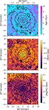 |
Fig. A.1. Stellar population maps of the central arc minute of M 74, extracted from the integrated (kinematic-corrected) data cube. From top to bottom: mean age, total metallicity [M/H] and [Mg/Fe] abundance. Masked regions are depicted in white and isophotal contours in black. The physical scale is given as a reference on the top X axis. |
All Tables
All Figures
|
Fig. 1. White image obtained combining the light in the full wavelength range of the cropped data cube of the central arc minute. |
| In the text | |
|
Fig. 2. From left to right, kinematic-corrected integrated data cube (given to C2D as an input), and the data cubes of the NSC, the bulge, and the disk. These three components are from the C2D spectrophotometric decomposition. Masked regions are plotted in black. |
| In the text | |
|
Fig. 3. Light ratio of each component over the total light of the galaxy, delivered by C2D. From left to right, NSC fitted as a PSF, bulge, and disk. The NSC dominates the light in the central spaxels within one PSF FWHM. Masked regions are plotted in white. |
| In the text | |
|
Fig. 4. Spectra obtained by integrating, within an aperture of 1σ of the PSF, the prepared kinematic-corrected (original) data cube before the spectrophotometric decomposition (blue solid), the NSC data cube (red dashed), and the host galaxy data cube (green dashed). Some spectral features, relevant for the stellar population analysis, are shown: Hβ, the Mgb triplet (not entirely resolved), and four Fe lines. |
| In the text | |
|
Fig. 5. Star formation histories of the NSC, the center of the host galaxy, and both components together (from the “original” MUSE data cube), from top to bottom. The three panels were plotted using the mass-weighted results from fitting spectra integrated in a central PSF aperture (Sect. 4.1.2 and Fig. 4). Mass fractions have been normalized to the mass of each component within the PSF aperture. The solid lines indicate the mean mass fraction for each age bin (half a billion year wide), calculated on the weight distributions from the 100 Monte Carlo realizations (Sect. 4.2). Dashed lines follow the median, and shades indicate the 16th and 84th percentiles from the distributions. |
| In the text | |
|
Fig. 6. Stellar population maps of the host galaxy component of M 74 after subtracting the NSC. From top to bottom, light-weighted age, total metallicity [M/H], and [Mg/Fe] abundance. The masked regions are depicted in white and isophotal contours in black. The physical scale is given as a reference in the top axis. |
| In the text | |
|
Fig. 7. Metallicity of the NSC as a function of the galaxy stellar mass (figure reconstructed and updated from Fig. 9 in Neumayer et al. 2020). The blue open circle indicates the [Fe/H] metallicity of the decomposed NSC of M 74. For comparison, [Fe/H] of the decomposed host galaxy is indicated with an open square, while a star indicates the [Fe/H] from the original (integrated) data cube of M 74 (see the text for all the details). The ETGs are indicated in red and LTGs in blue. Red circles are points from spectroscopic and photometric data (Koleva et al. 2009; Paudel et al. 2011; Spengler et al. 2017; Kacharov et al. 2018), as from Neumayer et al. (2020). The two solid black lines are the mass-metallicity relations of galaxies, given as reference, at the low-mass end (Kirby et al. 2013) and the high-mass end (Gallazzi et al. 2005). We have added the red triangles, which are NSC total metallicities ([M/H]) from Fahrion et al. (2021) and are therefore considered as upper limits for [Fe/H]. We have also added all the blue points. Blue triangles are for [M/H] and are thus upper limits of the NSCs in dwarf LTGs in Fahrion et al. (2022a). Blue circles are for the NSC [Fe/H] in more massive LTGs in Kacharov et al. (2018). |
| In the text | |
|
Fig. A.1. Stellar population maps of the central arc minute of M 74, extracted from the integrated (kinematic-corrected) data cube. From top to bottom: mean age, total metallicity [M/H] and [Mg/Fe] abundance. Masked regions are depicted in white and isophotal contours in black. The physical scale is given as a reference on the top X axis. |
| In the text | |
Current usage metrics show cumulative count of Article Views (full-text article views including HTML views, PDF and ePub downloads, according to the available data) and Abstracts Views on Vision4Press platform.
Data correspond to usage on the plateform after 2015. The current usage metrics is available 48-96 hours after online publication and is updated daily on week days.
Initial download of the metrics may take a while.