| Issue |
A&A
Volume 708, April 2026
|
|
|---|---|---|
| Article Number | A33 | |
| Number of page(s) | 8 | |
| Section | Extragalactic astronomy | |
| DOI | https://doi.org/10.1051/0004-6361/202558205 | |
| Published online | 25 March 2026 | |
A first look at a complete view of spatially resolved star formation at 1 < z < 1.8 with JWST NGDEEP+FRESCO slitless spectroscopy
1
Cosmic Dawn Center, Copenhagen, Denmark
2
Niels Bohr Institute, University of Copenhagen, Jagtvej 128, 2200, Copenhagen, Denmark
3
Max-Planck-Institut für Astronomie, Königstuhl 17, D-69117, Heidelberg, Germany
4
Department of Physics and Astronomy, Texas A&M University, College Station, TX 77843-4242, USA
5
George P. and Cynthia Woods Mitchell Institute for Fundamental Physics and Astronomy, Texas A&M University, College Station, TX 77845-4242, USA
6
Centro de Astrobiología (CAB), CSIC-INTA, Carretera de Ajalvir km 4, Torrejón de Ardoz, 28850, Madrid, Spain
7
Department of Astronomy, University of Geneva, Chemin Pegasi 51, 1290, Versoix, Switzerland
8
Department of Physics and Astronomy, University of California, Riverside, 900 University Avenue, Riverside, CA 92521, USA
9
Department of Astronomy, University of Washington, Seattle, WA 98195, USA
10
University of Massachusetts Amherst, 710 North Pleasant Street, Amherst, MA 01003-9305, USA
11
Astronomy Department, Yale University, 52 Hillhouse Ave, New Haven, CT 06511, USA
12
Department of Astronomy, The University of Texas at Austin, Austin, TX, USA
13
Cosmic Frontier Center, The University of Texas at Austin, Austin, TX 78712, USA
14
Space Telescope Science Institute, 3700 San Martin Drive, Baltimore, MD 21218, USA
15
Laboratory for Multiwavelength Astrophysics, School of Physics and Astronomy, Rochester Institute of Technology, 84 Lomb Memorial Drive, Rochester, NY 14623, USA
16
Institute of Science and Technology Austria (ISTA), Am Campus 1, A-3400, Klosterneuburg, Austria
17
Astronomy Centre, University of Sussex, Falmer, Brighton BN1 9QH, UK
18
Institute of Space Sciences and Astronomy, University of Malta, Msida MSD 2080, Malta
★ Corresponding author: This email address is being protected from spambots. You need JavaScript enabled to view it.
Received:
21
November
2025
Accepted:
27
February
2026
Abstract
The previously inaccessible star formation tracer Paschen-Alpha (Paα) can now be spatially resolved by JWST NIRCam slitless spectroscopy in distant galaxies up to cosmic noon. In the first study of its kind, we combine JWST NGDEEP NIRISS and FRESCO NIRCam slitless spectroscopy to provide the first direct comparison of spatially resolved dust-obscured (traced by Paα) versus unobscured (traced by Hα) star formation across the main sequence. We stacked Paα and Hα emission-line maps, along with stellar continuum images at both wavelengths of 31 galaxies at 1 < z < 1.8 in three bins of stellar mass spanning 7.7 ≤ log(M*/M⊙) < 11. Surface brightness profiles were measured and equivalent width (EW) profiles computed. Increasing Paα and Hα EW profiles with galactocentric radius across all stellar masses probed provides direct evidence for the inside-out growth of galaxies both via dust-obscured and unobscured star formation for the first time. For galaxies predominantly on the main sequence (log(M*/M⊙)≥8.8), a weakly positive (0.1 ± 0.1) Paα/Hα line profile gradient as a function of radius is found at 8.8 ≤ log(M*/M⊙) < 9.9, with a negative (−0.4 ± 0.1) Paα/Hα line profile gradient as a function of radius found at the highest stellar masses of 9.9 ≤ log(M*/M⊙) < 11.0. Low-mass galaxies (7.7 ≤ log(M*/M⊙) < 8.8) with predominantly high specific star formation rates relative to the main sequence are also found to have a negative (−0.5 ± 0.1) Paα/Hα line profile gradient as a function of radius. Our results demonstrate that while inside-out growth via star formation is ubiquitous across the main sequence just after cosmic noon, centrally concentrated dust attenuation is not. Along with other recent work in the literature, our findings now motivate future studies of resolved SFR and dust attenuation profiles in large samples of individual cosmic noon galaxies across the main sequence, aimed at understanding the intrinsic scatter in spatially resolved star formation.
Key words: galaxies: evolution / galaxies: formation / galaxies: high-redshift / galaxies: star formation / galaxies: stellar content / galaxies: structure
© The Authors 2026
 Open Access article, published by EDP Sciences, under the terms of the Creative Commons Attribution License (https://creativecommons.org/licenses/by/4.0), which permits unrestricted use, distribution, and reproduction in any medium, provided the original work is properly cited.
This article is published in open access under the Subscribe to Open model.
Open access funding provided by Max Planck Society.
1. Introduction
Understanding how galaxies build-up their stellar mass over cosmic time is a central goal in observational astrophysics, providing critical insight into how galaxies develop their structure. Tracking ongoing star formation in galaxies is therefore key to revealing the physical processes that regulate galaxy growth. Spatially resolving star formation in galaxies is the only way to determine where star formation occurs in galaxies, thereby revealing how galaxies assemble their stellar mass and evolve.
Multiple observational tracers spanning from the X-ray to the radio regime of the electromagnetic spectrum can be used to trace ongoing star formation in galaxies over various timescales. Of these, emission-line tracers provide a near-instantaneous measure of star formation due to their capability of tracing emission from the ionised gas surrounding massive young stars (Kennicutt et al. 1994; Kennicutt 1998; Kennicutt & Evans 2012 and references therein). The Hα emission line has been a popular choice for observing star formation in both nearby and distant galaxies due to its accessibility in the rest-frame optical and high intrinsic brightness. Spatially resolved Hα emission-line maps have revealed that from the end of reionisation (z ∼ 5.3) to z ∼ 0.5, galaxies grow ‘inside-out’ by forming new stars at progressively larger galactocentric radii over time (Nelson et al. 2012, 2016; Wilman et al. 2020; Matharu et al. 2022, 2024; Shen et al. 2024; Danhaive et al. 2025) but may experience centralised bursty star formation into the epoch of reionisation (Stephenson et al. 2025).
Despite the conveniences of using Hα as a star formation tracer, its susceptibility to dust attenuation leads to a systematic underestimation of star formation rates (SFRs; e.g. Whitaker et al. 2014; Shivaei et al. 2016). In cases of low to moderate dust attenuation, Hα-derived SFRs can be corrected using the Balmer decrement, whereby the Hα/Hβ flux ratio together with an assumed dust attenuation curve can be used to quantify the amount of dust attenuation towards star-forming regions (Calzetti et al. 2000; Osterbrock & Ferland 2006). Integrated Balmer decrements increase with stellar mass and SFR (Wild et al. 2011; Domínguez et al. 2013; Momcheva et al. 2013; Price et al. 2014; Reddy et al. 2015; Shivaei et al. 2015; Pirzkal et al. 2024; Sandles et al. 2024) but remain constant with redshift – a trend that is difficult to physically explain (Shapley et al. 2022, 2023). The few high-redshift (z ≥ 1) studies on spatially resolved Balmer decrements in typical star-forming galaxies find no shape evolution in the dust attenuation profiles with redshift at fixed stellar mass to help explain this trend, with predominantly centrally concentrated negative profiles found (Nelson et al. 2016; Matharu et al. 2023).
A gold standard alternative for obtaining a complete view of star formation in distant galaxies lies with the Paschen-Alpha (Paα) emission line. By virtue of being in the rest-frame near-infrared (NIR), it is insensitive to dust attenuation. Paα emission is therefore capable of tracing star formation in more heavily dust-obscured regions that would be optically thick to Balmer lines (Kennicutt & Evans 2012). Telluric OH emission, thermal emission, and its intrinsic faintness have made this line inaccessible to ground-based observatories. The Spitzer Space Telescope could access Paα in high-redshift galaxies, but only in rare cases of strong gravitational lensing (Papovich et al. 2009; Finkelstein et al. 2011; Shipley et al. 2016). Its rest-frame wavelength (1.875 μm) lies beyond the WFC3/IR wavelength regime covered by the Hubble Space Telescope (HST), making it inaccessible from space as well. Currently, with the launch of JWST, the Paα emission line has become accessible in multiple observational modes out to cosmic noon (NIRSpec slit spectroscopy: Reddy et al. 2023; NIRCam medium-band imaging: Williams et al. 2023; Suess et al. 2024; and NIRCam slitless spectroscopy: Liu et al. 2026; Neufeld et al. 2024). Evidence thus far suggests that Paα-derived SFRs could be ∼25% higher than those derived from dust-corrected Balmer line fluxes (Reddy et al. 2023), suggesting optically thick star formation in Hα. Liu et al. (2026) find that the SFR (Paα/Hα) increases with stellar mass, a result likely driven by increased dust extinction towards massive galaxies. At 1 < z < 1.6, the Paα versus stellar continuum effective radius is positive and increases with stellar mass, providing the first direct evidence for the inside-out growth of galaxies via dust-obscured star formation (Liu et al. 2026).
In this paper, we provide the first direct spatially resolved comparison of unobscured versus dust-obscured star formation using Hα and Paα emission-line maps for the same galaxies at 1 < z < 1.8 residing in the Hubble Ultra Deep Field (HUDF) using JWST NIRISS and NIRCam slitless spectroscopy from the Next Generation Deep Extragalactic Exploratory Public Survey (NGDEEP, Bagley et al. 2024, DOI) and the First Reionization Epoch Spectroscopically Complete Observations (FRESCO, Oesch et al. 2023, DOI). Our sample is described in Section 2, and our unique methodology for enabling direct comparisons between NIRCam and NIRISS slitless spectroscopy is detailed in Section 3. We outline our results in Section 4 and discuss their physical interpretations in Section 5. A summary of our findings is given in Section 6. All magnitudes quoted are in the AB system, logarithms are in base 10, and we assume a Lambda plus Cold Dark Matter (ΛCDM) cosmology with Ωm = 0.307, ΩΛ = 0.693, and H0 = 67.7 kms−1 Mpc−1 (Planck Collaboration XIII 2016).
2. Sample
In this section, we discuss various aspects of the sample used in our study. We describe the data (Section 2.1), how the Hα and Paα emission-line maps were generated (Section 2.2), and how the final sample was selected (Section 2.3 and 2.4).
2.1. Data and data processing
We used data from the JWST Cycle 1 programs NGDEEP and FRESCO. NGDEEP is a large treasury survey with 122.6 hours of NIRISS F115W, F150W, and F200W imaging and slitless spectroscopy centred on the HUDF, plus 96.4 hours of parallel NIRCam imaging of the HUDF-Par2 field – the deepest HST ACS F814W field on the sky. FRESCO is a medium survey with 53.8 hours of F444W NIRCam imaging and slitless spectroscopy of the GOODS-S and GOODS-N CANDELS fields. In this study, we used the NIRISS data from NGDEEP and the GOODS-S NIRCam data from FRESCO, which overlaps the HUDF (Figure 1). For more details on the NGDEEP and FRESCO surveys, we refer the reader to Bagley et al. (2024) and Oesch et al. (2023), respectively.
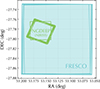 |
Fig. 1. FRESCO and NGDEEP NIRISS observing footprints overlaid on the sky. |
The Grism Redshift and Line Analysis Software (grizli; Brammer 2022) was used to process the imaging and slitless spectroscopy data together. grizli downloads and pre-processes the raw data from the Mikulski Archive for Space Telescopes (MAST). A basis set of template-flexible stellar population synthesis models (FSPS; Conroy et al. 2009; Conroy & Gunn 2010) is projected onto the pixel grid of the 2D grism exposures using spatial morphology from the imaging. Observed spectra are then fit with 2D template spectra with non-negative least squares. To break redshift degeneracies, a line complex template is used and the grism redshift is taken to be where the χ2 is minimised across the grid of trial redshifts input by the user. For full details on grizli, we refer the reader to Simons et al. (2021), Matharu et al. (2021) and Noirot et al. (2022, 2023).
2.2. Emission-line maps
The ∼2 − 4 times smaller bandwidths of the NIRISS filters and the order of magnitude lower resolving power of the NIRISS grisms (compared to F444W NIRCam) make the NGDEEP NIRISS slitless spectra significantly shorter than the FRESCO NIRCam slitless spectra. The standard grizli approach of forward-modelling the direct imaging to construct a contamination model for each 2D grism exposure is therefore computationally feasible for NIRISS grism observations and was used to process the NGDEEP NIRISS observations (see Shen et al. 2024 and references therein). Calibration files from Matharu & Brammer (2023) were used. For the grizli processing of FRESCO observations, grism spectra were instead median-filtered to remove the continuum (see Matharu et al. 2024 and references therein). Emission-line maps were created by inputting the wavelength of the line in the grizli-extraction process, which creates continuum-subtracted narrow-band maps given a specific wavelength.
2.3. Sample selection
The FRESCO grism spectra and grizli data products were visually inspected to verify Paα detections by the grizli software, as follows. Sources with Paα signal-to-noise ratio, S/N > 3 were initially selected from the grizli catalogue for visual inspection. Two inspectors independently assessed each using the SpecVizitor software1, classifying them into five categories based on line fit quality and redshift probability distribution: (1) contaminated, (2) no lines, (3) uncertain line fit quality, (4) robust single-line fit with consistent F444W morphology, and (5) robust multiple line fits. Sources flagged as robust (quality 4 or 5) by both reviewers were labelled ‘robust’; those flagged by only one were labelled ‘semi-robust’. A weighting scheme accounted for inspector bias where necessary. For this study, we selected robust (∼30%) and semi-robust (∼40%) sources, further limited to those with Paα S/N > 5, yielding a final catalogue of 508 robust Paα detections in GOODS-S. These detections were cross-matched with the 1153 Hα detections in the NGDEEP grizli extraction, yielding 43 matches. The NGDEEP grism spectra and grizli data products for this sample were visually inspected alongside the FRESCO grizli data products to verify the Hα detections and the quality of both the Hα and Paα emission-line maps. Thirty-five galaxies were identified with good quality Hα and Paα emission-line maps. For more details on the quality criteria for emission-line maps, we refer the reader to Section 2.3 of Matharu et al. (2024).
2.4. Stellar masses and star formation rates
The spectral energy distribution (SED) fitting code CIGALE (Boquien et al. 2019; Yang et al. 2020) was used to derive the stellar masses and SFRs for our galaxies in the NGDEEP NIRISS field. CANDELS (Koekemoer et al. 2011; Grogin et al. 2011) and JADES DR2 (Eisenstein et al. 2026; Rieke et al. 2023; Williams et al. 2023) photometry spanning 0.43–4.8 μm was used with the grism redshifts determined from the grizli NGDEEP extraction. The Calzetti et al. (2000) and Cardelli et al. (1989) dust laws with RV = 3.1 were used for attenuating the stellar continuum and emission-lines, respectively. Three active galactic nuclei (AGNs) were identified and removed from the sample by cross-matching with Lyu et al. (2022) with a 1 arcsecond radius. Active galactic nucleus activity can lead to Hα and Paα emission. Because we are only interested in studying star formation traced by Hα and Paα, we removed AGNs from our sample that would otherwise complicate the physical interpretation of our results as well as one galaxy for which we were unable to derive a stellar mass due to unavailable photometry. Our final sample consists of 31 galaxies. For full details on the SED fitting procedure – including a comparison of Hα versus SED-based SFRs – we refer the reader to Shen et al. (2025). A comparison of Paα versus SED-based SFRs can be found in Neufeld et al. (2024). The star formation main sequence (SFMS) of our final sample is shown in Figure 2, along with the three stellar mass bins (shaded grey regions) into which we divide our sample for subsequent analysis. The majority of the sample lies along the literature SFMS from Popesso et al. (2023) at the median redshift of our sample, indicating that we are primarily studying typical main-sequence galaxies at this redshift.
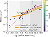 |
Fig. 2. SFMS of our sample measured using SED fitting (see Section 2.4). The shaded grey regions delineate our stellar mass bins for the stacking analysis. SFRs and the Popesso et al. (2023) SFMS include dust corrections. The dotted line indicates extrapolation. The brown line and orange region delineate the FRESCO Paα SFMS from Liu et al. (2026) and Neufeld et al. (2024), respectively. |
3. Methodology
In this section we describe how we prepare our data to enable the first direct comparison of Hα and Paα spatial profiles in the same galaxies at 1 < z < 1.8. This process involves the matching of PSFs between the two datasets (Section 3.1) as well as the stacking of imaging and emission-line maps (Section 3.2).
3.1. Point-spread function matching
The point spread function (PSF) of an instrument describes how light spreads on a detector for a point source, defining the resolution limit of the detector. The Hα and Paα emission-line maps used in our study were obtained from slitless spectroscopy taken with two different instruments on board JWST, which have different PSFs. Since the primary science goal of our study requires us to provide a direct comparison of the Hα and Paα spatial profiles in the same galaxies at these redshifts for the first time, the difference in PSFs must be accounted for. The PSF of a detector can be measured using observations of a star. The gold and blue lines in Figure 3 show the surface brightness profiles of the same star in the NGDEEP and FRESCO grizli direct-image thumbnails, both of which have identical pixel scale and orientation. Not only do the amplitudes differ (top panel), but so do the shapes – more explicitly shown in the bottom panel of Figure 3, where the profiles are peak-normalised.
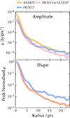 |
Fig. 3. PSF surface brightness profiles using the same star in F150W NGDEEP NIRISS and F444W FRESCO NIRCam imaging. The pink line indicates the PSF profile after matching (see Section 3.1) the FRESCO PSF to the NGDEEP PSF. The amplitude (top panel) of the PSF is maintained, and its shape (bottom panel) is appropriately altered. |
To address this problem, we PSF-matched the higher resolution FRESCO observations to the lower resolution NGDEEP observations. This was done by supplying pypher (Boucaud et al. 2016) with the direct-image thumbnails of the two stars in the same units to generate a matching kernel between the FRESCO and NGDEEP observations. The astropy package (Astropy Collaboration 2018) was then used to convolve the FRESCO F444W imaging and Paα maps with their respective matching kernels. The pink lines in Figure 3 show the result of this convolution on the FRESCO PSF profile. The amplitude of the FRESCO PSF is retained (top panel) while the shape is appropriately altered to match that of the NGDEEP PSF (bottom panel).
3.2. Stacking
To boost the signal-to-noise ratio as a function of galactocentric radius, we stacked the Hα and Paα emission-line maps and the direct imaging in three stellar mass bins: 7.7 ≤ Log(M*/M⊙) < 8.8, 8.8 ≤ Log(M*/M⊙) < 9.9, and 9.9 ≤ Log(M*/M⊙) < 11.0. Whilst Hα is predominantly detected within the F150W filter wavelength range for our sample, it is detected in the F200W wavelength range in a few cases. We therefore used the NGDEEP F150W and F200W grizli-generated thumbnails of the star used for the PSF matching (Section 3.1) between the two datasets to construct PSF stacks for our NGDEEP continuum and Hα stacks. Matching kernels were then created from the FRESCO F444W PSF to these PSF stacks, which were used to PSF-match (see Section 3.1) the F444W continuum and Paα stacks to the NGDEEP stacks. Full details of our stacking process can be found in Matharu et al. (2022). In summary, neighbouring sources were masked in both the direct image and emission-line map thumbnails using the grizli-generated segmentation map thumbnails for each galaxy. Pixels were weighted using the grizli-generated inverse variance map thumbnails, and each galaxy was weighted by its total flux in the corresponding direct image filter such that no single bright galaxy would dominate the stack. Direct image and emission-line map thumbnails were summed and exposure-corrected using the sum of their inverse variance maps. Each pixel is equal to 0.05 arcseconds, and the dimensions of all thumbnails and the final stacks are 160 × 160 pixels. Zoomed-in regions of our final Hα and PSF-matched Paα stacks can be seen in Figure 4.
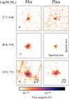 |
Fig. 4. Hα (first column) and Paα-to-NGDEEP convolved (second column) stacks for our sample in three stellar mass bins (rows). The number of galaxies within in each stack is shown in the bottom left corner of each Hα stack thumbnail. Each thumbnail is 60 × 60 pixels, with 1 pixel = 0.05″. Emission-line maps were generated such that the spectral axis is along the x-direction, while the y-direction is the spatial axis (see Section 3.3). |
3.3. Surface brightness profiles
Several recent studies have developed techniques to correct for the velocity effects on the morphologies of emission-line maps in the higher spectral resolution NIRCam grism spectroscopy (Li et al. 2023; Nelson et al. 2024; Danhaive et al. 2025). In our study, however, technical difficulties arose from the different spectral resolutions of the NIRCam and NIRISS grisms, instrument PSFs (see Section 3.1), source morphologies in the different filters, and detector properties. Robust measurements from our emission-line maps were therefore best obtained along the cross-dispersion axis, hereafter the ‘spatial axis’ (see Figure 4 and Matharu et al. 2024 for more details). The FRESCO observations in GOODS-S were taken at a position angle (PA) of zero (see Figure 1), aligning the spatial axis with the vertical axis of all grizli-processed imaging, grism spectroscopy, and emission-line maps. NGDEEP grizli data processing was run with a rotation to ensure that all final data products have PA = 0. Therefore, the spatial axis of the FRESCO emission-line maps and imaging directly correspond to the vertical axis of the NGDEEP emission-line maps and imaging. We hence measured surface brightness profiles along the central vertical strip of all our stacks with MAGPIE2. These profiles form the basis of our analysis in Section 4.
4. Results
Figure 5 shows the peak-normalised surface brightness profiles for the Hα, Paα, and PSF stacks along the central vertical strip of the spatial axis. The emission-line map profiles are consistently more extended than their PSF profiles, demonstrating that they are all spatially resolved by JWST NIRCam and NIRISS. For our lowest- and highest-mass bins, the Hα emission is more extended than the Paα emission. Whereas for our middle mass bin, Hα and Paα have similar spatial profiles out to ∼2 kpc after which Paα emission is more extended than the Hα emission out to 3 kpc.
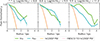 |
Fig. 5. Peak-normalised Hα (green) and Paα (turquoise) surface brightness profiles for our stacks shown in Figure 4. Both profiles are more extended than their PSFs, demonstrating that they are well resolved. At the lowest and highest masses, the Hα emission is more extended than the Paα emission, whereas their spatial profiles are similar for our middle stellar mass bin, at least out to ∼2 kiloparsecs after which the Paα emission is more extended than the Hα emission. |
We show the quotient of the emission-line map profiles with their respective continuum profiles in Figure 6. Known as the equivalent width (EW), this quantity provides an absolute measurement for the strength of the emission line. We use the Kendall’s Tau (τ) statistic to measure the correlation between the EW and radius. Errors on τ were computed using Monte Carlo sampling by drawing 1000 random samples from each line profile and their errors from a normal distribution with a standard deviation equal to the measurement errors. The error on τ thus represents the standard deviation of the 1000 τ measurements obtained. Both EW(Hα) and EW(Paα) have positive profile gradients as a function of radius for all stellar mass bins. The equivalent width of Paα consistently exhibits higher normalisation than EW(Hα).
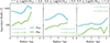 |
Fig. 6. Paα (turquoise) and Hα (green) EW profiles for our stacks, with their Kendall’s Tau (τ) correlation statistics. All EW profiles display a positive radial gradient, demonstrating that star-forming galaxies at these redshifts and stellar masses are growing inside-out both via dust-obscured (Paα) and unobscured (Hα) star formation. |
Figure 7 shows the emission line flux profiles for our Hα and Paα stacks and their ratios. As demonstrated by the τ statistic, our Paα/Hα profiles have negative gradients with increasing radius for the lowest and highest stellar mass bins, but a mildly positive gradient with increasing radius for our middle stellar mass bin. In the next section, we discuss the physical interpretation of our results.
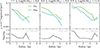 |
Fig. 7. Surface brightness profiles for our Hα (green) and Paα (turquoise) stacks (top row) with their ratios (bottom row) and Kendall’s Tau (τ) correlation statistics. The horizontal dotted line shows the expected Paα/Hα line ratio for Case B recombination (Te = 10 000 K and ne = 100 cm−3 based on photoionisation modelling with CLOUDY (Ferland et al. 2017)). Declining Paα/Hα with galactocentric radius in our highest- and lowest-mass bins highlights the additional dust-obscured star formation that Paα traces closer to galactic centres, which decreases towards the outskirts. |
5. Discussion
The most massive and short-lived (∼10 Myr) O-type stars emit the strongest ultraviolet (UV) radiation, capable of stripping hydrogen atoms of their electrons. The recombination of these electrons with ionised hydrogen atoms further from the centre of these stars leads to the emission of hydrogen recombination lines such as Hα in the rest-frame optical and Paα in the rest-frame NIR. Whilst the Hα emission line is intrinsically stronger than the Paα emission line – and therefore more than eight times brighter (Case B recombination, Te = 104 K) – it is more susceptible to dust attenuation. Therefore, Hα is often regarded as a good tracer of unobscured ongoing star formation only. Paα is dubbed a ‘gold standard’ tracer of ongoing star formation due to its capability in tracing more heavily dust-obscured ongoing star formation (Kennicutt & Evans 2012).
5.1. Galaxy growth
The EW profiles of these emission lines (Figure 6) measure their strength with respect to their underlying continuum as a function of galactocentric radius. The normalisation of both EW profiles decrease with increasing stellar mass, consistent with the decrease in sSFRs (Popesso et al. 2023 and references therein) and the increasing contribution of older stellar populations to the stellar continuum both in the optical and NIR. In general, all EW profiles are positive for all three stellar mass bins, providing direct evidence for the inside-out growth of galaxies via star formation after cosmic noon, confirmed here for the first time with both Hα and Paα (see also Liu et al. 2026 for Paα vs continuum-size analysis).
Areas often missed in EW(Hα) profiles are either optically thick regions at the rest-frame Hα wavelength (6565Å) or regions with higher nebular dust attenuation, which reduces the Hα line flux more than the stellar attenuation reduces the continuum flux. In the first case, both the Hα line flux and continuum are affected. The second case applies to star-forming regions (e.g. Calzetti et al. 2000; Förster Schreiber et al. 2009; Yoshikawa et al. 2010; Mancini et al. 2011; Wuyts et al. 2011, 2013; Kashino et al. 2013; Kreckel et al. 2013; Price et al. 2014; Reddy et al. 2015; Bassett et al. 2017; Theios et al. 2019; Koyama et al. 2019; Greener et al. 2020; Wilman et al. 2020; Rodríguez-Muñoz et al. 2021) and leads to an underestimation of EW(Hα). In the next section, we therefore discuss a cleaner approach to comparing unobscured versus obscured star formation using our measurements.
5.2. Unobscured versus obscured star formation
It is impossible to gain deeper insight into spatially resolved unobscured versus obscured star formation by directly comparing Hα and Paα EW profiles. This is because of complications introduced by differential dust attenuation of the Hα line and the continuum at 6565 Å (see Section 5.1), as well as differing relative contributions of different stellar populations to the continuum in the rest-frame optical versus the NIR. We therefore instead directly compare the Hα and Paα line profiles with their ratios in Figure 7. On average, line flux increases with stellar mass in line with increasing SFRs along the main sequence (see Figure 2). In the lowest- and highest-mass bins, the Paα/Hα profiles decline with radius from the centre towards the expected Paα/Hα value in the absence of dust attenuation (horizontal dotted line; Case B recombination, Te = 10 000 K and ne = 100 cm−3, based on photoionisation modelling with CLOUDY (Ferland et al. 2017)). In our lowest-mass bin, we predominantly probe galaxies with high sSFRs and in our highest-mass bin, those with the highest SFRs (see Figure 2). This trend in the Paα/Hα profiles suggests that the dust in the central regions of these galaxies preferentially attenuates the Hα flux relative to the Paα flux. Our result at the highest stellar masses is consistent with many ALMA studies (see discussion in Shen et al. 2023) and recent JWST MIRI imaging results from Shen et al. (2023) and Magnelli et al. (2023). The rate of galaxy growth via star formation with radius measured using Hα emission alone in the central regions (∼1.5 kpc) of such galaxies could therefore be overestimated.
In contrast, the relatively flat Paα/Hα line profile of the main-sequence galaxies in our middle mass bin suggests that not all main-sequence galaxies at cosmic noon growing inside-out via star formation have centrally concentrated dust attenuation. This more complicated star formation history (SFH) for the central and outer regions of galaxies is supported by the recent results of Shen et al. (2024), who examined spatially resolved EW(Hα), sSFRs, and ages for 19 main-sequence galaxies at 0.6 < z < 2.2 with comparable stellar masses (9 ≤ Log(M*/M⊙) < 11) to our sample in the same NGDEEP NIRISS field (see also Matharu et al. 2023; Liu et al. 2023, 2026; Maheson et al. 2025). Whilst the majority (84%) of their galaxies show positive EW(Hα) profiles supporting the inside-out growth scenario, the sSFR and SFH profiles suggest at least one rapid star formation episode forming the bulge; nevertheless, smoothly varying SFHs for the disk indicates longer timescale inside-out growth. Our results along with those of Shen et al. (2024) put forth a more complex picture for spatially resolved star formation at and around cosmic noon. Large-sample resolved studies of individual galaxies at cosmic noon across the main sequence are now required to understand the intrinsic scatter in how star formation progresses in galaxies.
6. Summary
By processing overlapping JWST NGDEEP NIRISS and FRESCO NIRCam slitless spectroscopy in the HUDF, we provided the first direct comparison of spatially resolved unobscured (traced by Hα) and dust-obscured (traced by Paα) ongoing star formation in 31 galaxies at 1 < z < 1.8 (Section 4). Our main conclusions are listed below.
-
Positive EW(Paα) and EW(Hα) profiles demonstrate that main-sequence galaxies just after cosmic noon grow inside-out both via dust-obscured and unobscured star formation.
-
At the highest stellar masses and sSFRs, Paα/Hα decreases with increasing galactocentric radius, likely tracing decreasing dust-obscured star formation relative to unobscured star formation towards larger radii.
-
The relatively flat Paα/Hα line profile for our stack of galaxies with stellar masses 8.8 ≤ log(M*/M⊙) < 9.9 suggests that centrally concentrated dust attenuation is not ubiquitous across the main sequence just after cosmic noon in galaxies growing inside-out via star formation.
Our work puts forth a proof-of-concept for combining NIRISS and NIRCam slitless spectroscopy to accomplish more detailed resolved studies of high-redshift galaxies. Together with similar studies in the literature, this motivates a strong case for detailed, resolved studies of large samples of individual galaxies across the main sequence at cosmic noon to understand the intrinsic scatter in spatially resolved star formation.
Acknowledgments
JM is grateful to the Max Planck Society for the MPIA Prize Fellowship and to the Cosmic Dawn Center for the DAWN Fellowship. This work is based on observations made with the NASA/ESA/CSA James Webb Space Telescope. The raw data were obtained from the Mikulski Archive for Space Telescopes at the Space Telescope Science Institute, which is operated by the Association of Universities for Research in Astronomy, Inc., under NASA contract NAS 5-03127 for JWST. These observations are associated with JWST Cycle 1 GO programs #1895 and #2079. Support for both programs was provided by NASA through a grant from the Space Telescope Science Institute, which is operated by the Associations of Universities for Research in Astronomy, Incorporated, under NASA contract NAS5-26555. The Cosmic Dawn Center (DAWN) is funded by the Danish National Research Foundation under grant DNRF140. This work has received funding from the Swiss State Secretariat for Education, Research and Innovation (SERI) under contract number MB22.00072, as well as from the Swiss National Science Foundation (SNSF) through project grant 200020_207349. This work benefited from support from the George P. and Cynthia Woods Mitchell Institute for Fundamental Physics and Astronomy at Texas A&M University. CP thanks Marsha and Ralph Schilling for generous support of this research.
References
- Astropy Collaboration (Price-Whelan, A. M., et al.) 2018, AJ, 156, 123 [Google Scholar]
- Bagley, M. B., Pirzkal, N., Finkelstein, S. L., et al. 2024, ApJ, 965, L6 [NASA ADS] [CrossRef] [Google Scholar]
- Bassett, R., Glazebrook, K., Fisher, D. B., et al. 2017, MNRAS, 467, 239 [NASA ADS] [Google Scholar]
- Boquien, M., Burgarella, D., Roehlly, Y., et al. 2019, A&A, 622, A103 [NASA ADS] [CrossRef] [EDP Sciences] [Google Scholar]
- Boucaud, A., Bocchio, M., Abergel, A., et al. 2016, A&A, 596, A63 [NASA ADS] [CrossRef] [EDP Sciences] [Google Scholar]
- Brammer, G. 2022, https://doi.org/10.5281/zenodo.7351572 [Google Scholar]
- Calzetti, D., Armus, L., Bohlin, R. C., et al. 2000, ApJ, 533, 682 [NASA ADS] [CrossRef] [Google Scholar]
- Cardelli, J. A., Clayton, G. C., & Mathis, J. S. 1989, ApJ, 345, 245 [Google Scholar]
- Conroy, C., & Gunn, J. E. 2010, ApJ, 712, 833 [Google Scholar]
- Conroy, C., Gunn, J. E., & White, M. 2009, ApJ, 699, 486 [Google Scholar]
- Danhaive, A. L., Tacchella, S., McClymont, W., et al. 2025, MNRAS, submitted, [arXiv:2510.06315] [Google Scholar]
- Domínguez, A., Siana, B., Henry, A. L., et al. 2013, ApJ, 763, 145 [CrossRef] [Google Scholar]
- Eisenstein, D. J., Willott, C., Alberts, S., et al. 2026, ApJS, 283, 6 [Google Scholar]
- Ferland, G. J., Chatzikos, M., Guzmán, F., et al. 2017, Rev. Mex. Astron. Astrofis., 53, 385 [NASA ADS] [Google Scholar]
- Finkelstein, K. D., Papovich, C., Finkelstein, S. L., et al. 2011, ApJ, 742, 108 [CrossRef] [Google Scholar]
- Förster Schreiber, N. M., Genzel, R., Bouché, N., et al. 2009, ApJ, 706, 1364 [Google Scholar]
- Greener, M. J., Aragón-Salamanca, A., Merrifield, M. R., et al. 2020, MNRAS, 495, 2305 [CrossRef] [Google Scholar]
- Grogin, N. A., Kocevski, D. D., Faber, S. M., et al. 2011, ApJS, 197, 35 [NASA ADS] [CrossRef] [Google Scholar]
- Kashino, D., Silverman, J. D., Rodighiero, G., et al. 2013, ApJ, 777, 4 [Google Scholar]
- Kennicutt, R. C., Jr 1998, ARA&A, 36, 189 [NASA ADS] [CrossRef] [Google Scholar]
- Kennicutt, R. C., & Evans, N. J. 2012, ARAA, 50, 531 [NASA ADS] [CrossRef] [Google Scholar]
- Kennicutt, R. C., Jr, Tamblyn, P., & Congdon, C. E. 1994, ApJ, 435, 22 [NASA ADS] [CrossRef] [Google Scholar]
- Koekemoer, A. M., Faber, S. M., Ferguson, H. C., et al. 2011, ApJS, 197, 36 [NASA ADS] [CrossRef] [Google Scholar]
- Koyama, Y., Shimakawa, R., Yamamura, I., Kodama, T., & Hayashi, M. 2019, PASJ, 71, 1 [NASA ADS] [CrossRef] [Google Scholar]
- Kreckel, K., Groves, B., Schinnerer, E., et al. 2013, ApJ, 771, 62 [NASA ADS] [CrossRef] [Google Scholar]
- Li, Z., Cai, Z., Sun, F., et al. 2023, ApJ, submitted, [arXiv:2310.09327] [Google Scholar]
- Liu, Z., Morishita, T., & Kodama, T. 2023, ApJ, 955, 29 [NASA ADS] [CrossRef] [Google Scholar]
- Liu, Z., Morishita, T., & Kodama, T. 2026, ApJ, 998, 203 [Google Scholar]
- Lyu, J., Alberts, S., Rieke, G. H., & Rujopakarn, W. 2022, ApJ, 941, 191 [NASA ADS] [CrossRef] [Google Scholar]
- Magnelli, B., Gómez-Guijarro, C., Elbaz, D., et al. 2023, A&A, 678, A83 [NASA ADS] [CrossRef] [EDP Sciences] [Google Scholar]
- Maheson, G., Tacchella, S., Belli, S., et al. 2025, MNRAS, submitted, [arXiv:2504.15346] [Google Scholar]
- Mancini, C., Förster Schreiber, N. M., Renzini, A., et al. 2011, ApJ, 743, 86 [CrossRef] [Google Scholar]
- Matharu, J., & Brammer, G. 2023, https://doi.org/10.5281/zenodo.7628094 [Google Scholar]
- Matharu, J., Muzzin, A., Brammer, G. B., et al. 2021, ApJ, 923, 222 [NASA ADS] [CrossRef] [Google Scholar]
- Matharu, J., Papovich, C., Simons, R. C., et al. 2022, ApJ, 937, 16 [NASA ADS] [CrossRef] [Google Scholar]
- Matharu, J., Muzzin, A., Sarrouh, G. T. E., et al. 2023, ApJ, 949, L11 [NASA ADS] [CrossRef] [Google Scholar]
- Matharu, J., Nelson, E. J., Brammer, G., et al. 2024, A&A, 690, A64 [NASA ADS] [CrossRef] [EDP Sciences] [Google Scholar]
- Momcheva, I. G., Lee, J. C., Ly, C., et al. 2013, AJ, 145, 47 [NASA ADS] [CrossRef] [Google Scholar]
- Nelson, E. J., Van Dokkum, P. G., Brammer, G., et al. 2012, ApJ, 747, 6 [Google Scholar]
- Nelson, E. J., van Dokkum, P. G., Förster Schreiber, N. M., et al. 2016, ApJ, 828, 27 [Google Scholar]
- Nelson, E. J., van Dokkum, P. G., Momcheva, I. G., et al. 2016, ApJ, 817, L9 [CrossRef] [Google Scholar]
- Nelson, E., Brammer, G., Giménez-Arteaga, C., et al. 2024, ApJ, 976, L27 [NASA ADS] [CrossRef] [Google Scholar]
- Neufeld, C., van Dokkum, P., Asali, Y., et al. 2024, ApJ, 972, 156 [Google Scholar]
- Noirot, G., Sawicki, M., Abraham, R., et al. 2022, MNRAS, 512, 3566 [NASA ADS] [CrossRef] [Google Scholar]
- Noirot, G., Desprez, G., Asada, Y., et al. 2023, MNRAS, 525, 1867 [NASA ADS] [CrossRef] [Google Scholar]
- Oesch, P. A., Brammer, G., Naidu, R. P., et al. 2023, MNRAS, 525, 2864 [NASA ADS] [CrossRef] [Google Scholar]
- Osterbrock, D. E., & Ferland, G. J. 2006, Astrophysics of gaseous nebulae and active galactic nuclei(Sausalito, CA: University Science Books) [Google Scholar]
- Papovich, C., Rudnick, G., Rigby, J. R., et al. 2009, ApJ, 704, 1506 [CrossRef] [Google Scholar]
- Pirzkal, N., Rothberg, B., Papovich, C., et al. 2024, ApJ, 969, 90 [Google Scholar]
- Planck Collaboration XIII. 2016, A&A, 594, A13 [NASA ADS] [CrossRef] [EDP Sciences] [Google Scholar]
- Popesso, P., Concas, A., Cresci, G., et al. 2023, MNRAS, 519, 1526 [Google Scholar]
- Price, S. H., Kriek, M., Brammer, G. B., et al. 2014, ApJ, 788, 86 [NASA ADS] [CrossRef] [Google Scholar]
- Reddy, N. A., Kriek, M., Shapley, A. E., et al. 2015, ApJ, 806, 259 [NASA ADS] [CrossRef] [Google Scholar]
- Reddy, N. A., Topping, M. W., Sanders, R. L., Shapley, A. E., & Brammer, G. 2023, ApJ, 948, 83 [NASA ADS] [CrossRef] [Google Scholar]
- Rieke, M. J., Robertson, B., Tacchella, S., et al. 2023, ApJS, 269, 16 [NASA ADS] [CrossRef] [Google Scholar]
- Rodríguez-Muñoz, L., Rodighiero, G., Pérez-González, P. G., et al. 2021, MNRAS, 510, 2061 [CrossRef] [Google Scholar]
- Sandles, L., D’Eugenio, F., Maiolino, R., et al. 2024, A&A, 691, A305 [NASA ADS] [CrossRef] [EDP Sciences] [Google Scholar]
- Shapley, A. E., Sanders, R. L., Salim, S., et al. 2022, ApJ, 926, 145 [NASA ADS] [CrossRef] [Google Scholar]
- Shapley, A. E., Sanders, R. L., Reddy, N. A., Topping, M. W., & Brammer, G. B. 2023, ApJ, 954, 157 [NASA ADS] [CrossRef] [Google Scholar]
- Shen, L., Papovich, C., Yang, G., et al. 2023, ApJ, 950, 7 [NASA ADS] [CrossRef] [Google Scholar]
- Shen, L., Papovich, C., Matharu, J., et al. 2024, ApJ, 963, L49 [NASA ADS] [CrossRef] [Google Scholar]
- Shen, L., Papovich, C., Matharu, J., et al. 2025, ApJ, 980, L45 [Google Scholar]
- Shipley, H. V., Papovich, C., Rieke, G. H., Brown, M. J. I., & Moustakas, J. 2016, ApJ, 818, 60 [NASA ADS] [CrossRef] [Google Scholar]
- Shivaei, I., Reddy, N. A., Shapley, A. E., et al. 2015, ApJ, 815, 98 [NASA ADS] [CrossRef] [Google Scholar]
- Shivaei, I., Kriek, M., Reddy, N. A., et al. 2016, ApJ, 820, L23 [NASA ADS] [CrossRef] [Google Scholar]
- Simons, R. C., Papovich, C., Momcheva, I., et al. 2021, ApJ, 923, 203 [NASA ADS] [CrossRef] [Google Scholar]
- Stephenson, H. M. O., Stott, J. P., Pirie, C. A., et al. 2025, MNRAS, 544, 1412 [Google Scholar]
- Suess, K. A., Weaver, J. R., Price, S. H., et al. 2024, ApJ, 976, 101 [Google Scholar]
- Theios, R. L., Steidel, C. C., Strom, A. L., et al. 2019, ApJ, 871, 128 [NASA ADS] [CrossRef] [Google Scholar]
- Whitaker, K. E., Franx, M., Leja, J., et al. 2014, ApJ, 795, 104 [NASA ADS] [CrossRef] [Google Scholar]
- Wild, V., Charlot, S., Brinchmann, J., et al. 2011, MNRAS, 417, 1760 [NASA ADS] [CrossRef] [Google Scholar]
- Williams, C. C., Tacchella, S., Maseda, M. V., et al. 2023, ApJS, 268, 64 [NASA ADS] [CrossRef] [Google Scholar]
- Wilman, D. J., Fossati, M., Mendel, J. T., et al. 2020, ApJ, 892, 1 [NASA ADS] [CrossRef] [Google Scholar]
- Wuyts, S., Förster Schreiber, N. M., Lutz, D., et al. 2011, ApJ, 738, 106 [Google Scholar]
- Wuyts, S., Förster Schreiber, N. M., Nelson, E. J., et al. 2013, ApJ, 779, 135 [Google Scholar]
- Yang, F., Long, R. J., Shan, S.-S., et al. 2020, MNRAS, 5, 1 [Google Scholar]
- Yoshikawa, T., Akiyama, M., Kajisawa, M., et al. 2010, ApJ, 718, 112 [NASA ADS] [CrossRef] [Google Scholar]
All Figures
|
Fig. 1. FRESCO and NGDEEP NIRISS observing footprints overlaid on the sky. |
| In the text | |
|
Fig. 2. SFMS of our sample measured using SED fitting (see Section 2.4). The shaded grey regions delineate our stellar mass bins for the stacking analysis. SFRs and the Popesso et al. (2023) SFMS include dust corrections. The dotted line indicates extrapolation. The brown line and orange region delineate the FRESCO Paα SFMS from Liu et al. (2026) and Neufeld et al. (2024), respectively. |
| In the text | |
|
Fig. 3. PSF surface brightness profiles using the same star in F150W NGDEEP NIRISS and F444W FRESCO NIRCam imaging. The pink line indicates the PSF profile after matching (see Section 3.1) the FRESCO PSF to the NGDEEP PSF. The amplitude (top panel) of the PSF is maintained, and its shape (bottom panel) is appropriately altered. |
| In the text | |
|
Fig. 4. Hα (first column) and Paα-to-NGDEEP convolved (second column) stacks for our sample in three stellar mass bins (rows). The number of galaxies within in each stack is shown in the bottom left corner of each Hα stack thumbnail. Each thumbnail is 60 × 60 pixels, with 1 pixel = 0.05″. Emission-line maps were generated such that the spectral axis is along the x-direction, while the y-direction is the spatial axis (see Section 3.3). |
| In the text | |
|
Fig. 5. Peak-normalised Hα (green) and Paα (turquoise) surface brightness profiles for our stacks shown in Figure 4. Both profiles are more extended than their PSFs, demonstrating that they are well resolved. At the lowest and highest masses, the Hα emission is more extended than the Paα emission, whereas their spatial profiles are similar for our middle stellar mass bin, at least out to ∼2 kiloparsecs after which the Paα emission is more extended than the Hα emission. |
| In the text | |
|
Fig. 6. Paα (turquoise) and Hα (green) EW profiles for our stacks, with their Kendall’s Tau (τ) correlation statistics. All EW profiles display a positive radial gradient, demonstrating that star-forming galaxies at these redshifts and stellar masses are growing inside-out both via dust-obscured (Paα) and unobscured (Hα) star formation. |
| In the text | |
|
Fig. 7. Surface brightness profiles for our Hα (green) and Paα (turquoise) stacks (top row) with their ratios (bottom row) and Kendall’s Tau (τ) correlation statistics. The horizontal dotted line shows the expected Paα/Hα line ratio for Case B recombination (Te = 10 000 K and ne = 100 cm−3 based on photoionisation modelling with CLOUDY (Ferland et al. 2017)). Declining Paα/Hα with galactocentric radius in our highest- and lowest-mass bins highlights the additional dust-obscured star formation that Paα traces closer to galactic centres, which decreases towards the outskirts. |
| In the text | |
Current usage metrics show cumulative count of Article Views (full-text article views including HTML views, PDF and ePub downloads, according to the available data) and Abstracts Views on Vision4Press platform.
Data correspond to usage on the plateform after 2015. The current usage metrics is available 48-96 hours after online publication and is updated daily on week days.
Initial download of the metrics may take a while.