| Issue |
A&A
Volume 708, April 2026
|
|
|---|---|---|
| Article Number | A100 | |
| Number of page(s) | 11 | |
| Section | Extragalactic astronomy | |
| DOI | https://doi.org/10.1051/0004-6361/202558215 | |
| Published online | 01 April 2026 | |
Exploring the ultra-faint dwarf Boötes I using JWST and HST: Metallicity distribution and binaries
1
Dipartimento di Fisica e Astronomia “Galileo Galilei”, Università Degli Studi di Padova, Vicolo dell’Osservatorio 3, 35122 Padova, Italia
2
Istituto Nazionale di Astrofisica – Osservatorio Astronomico di Padova, Vicolo dell’Osservatorio 5, 35122 Padova, Italy
3
Dipartimento di Tecnica e Gestione dei Sistemi Industriali, Università degli Studi di Padova, Stradella S. Nicola 3, I-36100 Vicenza, Italy
4
Research School of Astronomy and Astrophysics, Australian National University, Canberra, ACT 2611, Australia
5
South-Western Institute for Astronomy Research, Yunnan University, Kunming 650500, PR China
★ Corresponding author: This email address is being protected from spambots. You need JavaScript enabled to view it.
Received:
21
November
2025
Accepted:
27
February
2026
Abstract
Ultra-faint dwarf galaxies (UFDs) are among the oldest and most metal-poor stellar systems in the Universe. Their metallicity distribution encodes the fossil record of the earliest star formation, feedback, and chemical enrichment, providing crucial tests of models of the first stars, galaxy assembly, and dark matter halos. However, due to their faint luminosities and the limited number of bright giants, spectroscopic studies of UFDs typically probe only small stellar samples. Here, we present an analysis of multi-epoch Hubble Space Telescope and James Webb Space Telescope observations of the UFD Boötes I. Using a deep color–magnitude diagram in the F606W and F322W2 bands, extending from the subgiant branch to the M dwarfs, and stellar proper motions to identify likely members, we obtained an unprecedentedly clean census of the system. The exquisite quality of the diagram, combined with the sensitivity of M-dwarf colors to metallicity, allowed us to constrain the metallicity distribution in a large stellar sample. As a first step, we then exploited the metallicity sensitivity of M-dwarf colors to derive the metallicity distribution function. We find that most of the stars ∼85% have [Fe/H] < −2, and that roughly ∼17% have [Fe/H] < − 3. Then, we derived the binary fraction in Boötes I. This is crucial since binaries can bias kinematic mass estimates, affect stellar population analyzes, and shape the photometric signatures used to infer metallicity. We find that 20 ± 2% of stellar systems in Boötes I are binaries with mass ratios larger than 0.4, corresponding to a total binary fraction of ∼30%. This value is comparable to the binary fractions observed in globular clusters of similar stellar mass, suggesting that the presence of dark matter does not significantly affect the binary properties of Boötes I.
Key words: stars: abundances / binaries: close / Hertzsprung-Russell and C-M diagrams / galaxies: abundances / galaxies: dwarf
© The Authors 2026
 Open Access article, published by EDP Sciences, under the terms of the Creative Commons Attribution License (https://creativecommons.org/licenses/by/4.0), which permits unrestricted use, distribution, and reproduction in any medium, provided the original work is properly cited.
This article is published in open access under the Subscribe to Open model. This email address is being protected from spambots. You need JavaScript enabled to view it. to support open access publication.
1. Introduction
Ultra-faint dwarf galaxies (UFDs) are among the oldest and most chemically primitive stellar systems known, typically defined as having total luminosities below 105 L⊙ (e.g., Simon 2019, and references therein). Over the past two decades, numerous UFDs have been identified through wide-field imaging surveys (e.g., Belokurov et al. 2010; Willman et al. 2011; Kim et al. 2015). Although they may superficially resemble globular clusters (GCs), UFDs display distinctive structural and dynamical properties that clearly distinguish them as separate systems.
One of the most intriguing features of UFDs is their extreme dark matter content: their total dynamical masses exceed stellar mass by factors of 102–104, corresponding to mass-to-light ratios of similar magnitude (e.g., Simon & Geha 2007; McConnachie 2012; Battaglia & Nipoti 2022). Owing to their relative proximity, UFDs represent unique laboratories for probing the nature and distribution of dark matter on the smallest galactic scales. Moreover, due to their extremely low baryonic content and their residence in low-mass dark matter-dominated halos, UFDs represent ideal laboratories for constraining the nature of dark matter (Zoutendijk et al. 2021) and for testing models proposed to explain the missing satellite problem (Simon 2019). Furthermore, deep Hubble Space Telescope (HST) observations have shown that the stellar populations of UFDs are predominantly ancient, supporting the view that they are “fossil” galaxies–systems that formed most of their stars before reionization and subsequently ceased to form stars (e.g., Brown et al. 2014; Sacchi et al. 2021; Savino et al. 2023; Durbin et al. 2025).
Reliable estimates of the dark matter content in UFDs are currently obtained from measurements of the radial–velocity dispersion of their member stars. Early studies already indicated that UFDs contain a large amount of dark matter based on their unexpectedly high velocity dispersions. More recent work on Boötes I and Leo IV reported dispersions of 4 − 5 km s−1 and ∼3 km s−1respectively, supporting the presence of a dark matter halo (e.g., Jenkins et al. 2021; Longeard et al. 2022; Sandford et al. 2025).
However, unresolved binary systems can artificially inflate the observed velocity dispersion, leading to overestimates of the inferred dark matter mass (Spencer et al. 2018; Pianta et al. 2022). Consequently, constraining the binary fraction and the properties of binary stars is essential to obtain robust dynamical measurements (Spencer et al. 2017, 2018; McConnachie & Côté 2010; Gration et al. 2025).
Another intriguing characteristic of UFDs is the considerable variation in iron (Fe) and α-element abundances observed among their stars, interpreted as the result of extended star formation episodes and internal chemical enrichment (Simon & Geha 2007; Kirby et al. 2008). These chemical patterns contrast sharply with those seen in GCs, which generally display much smaller star-to-star metallicity variations (e.g., Marino et al. 2015; Legnardi et al. 2022), resembling those observed in brighter dwarf galaxies. At the same time, UFDs are less complex than massive galaxies, making them ideal laboratories for studying the fundamental mechanisms that govern chemical evolution in low-mass galaxies. However, metallicity determinations mostly rely on spectroscopy of red giant branch (RGB) stars, which are typically few in number (Norris et al. 2010a; Lai et al. 2011; Frebel et al. 2016). This limitation arises from the sensitivity of current telescopes, which cannot obtain high-resolution spectra for faint stars, combined with the sparsely populated RGBs characteristic of most UFDs.
In this paper, we take advantage of imaging data collected with the HST and the James Webb Space Telescope (JWST) to study Boötes I, one of the most extensively investigated UFDs. The resulting high-precision photometry enables us to pursue two main goals: (i) the determination of the metallicity distribution, and (ii) the characterization of the binary fraction along the main sequence (MS).
Discovered by Belokurov et al. (2006), Boötes I has since been the subject of numerous investigations of its stellar populations and chemical composition. With a luminosity of LV = 2.8 × 10⁴ L⊙, Boötes I is among the brightest known UFDs. Using the Ca II K line–strength index, Norris et al. (2008) reported a mean [Fe/H] of −2.51 ± 0.13 for a sample of 16 stars. Further high-resolution spectroscopic studies have confirmed a mean value of ⟨[Fe/H]⟩≃ − 2.6, a wide iron range of ∼2 dex, and very metal-poor stars with [Fe/H] < −3.5 (Norris et al. 2010b; Koposov et al. 2011; Gilmore et al. 2013; Ishigaki et al. 2014). Similar results were also inferred using low- to medium-resolution spectroscopy (Lai et al. 2011; Jenkins et al. 2021; Longeard et al. 2022; Sandford et al. 2025). As noted above, Boötes I exhibits a relatively large line-of-sight velocity dispersion, implying a high mass-to-light ratio and a significant dark matter component.
Boötes I is composed of old stellar populations and hosts a conspicuous fraction of binaries. From an analysis of the color-magnitude diagram (CMD) based on HST data, Brown et al. (2014, see also Durbin et al. 2025) inferred an age of about 13 Gyr, while Gennaro et al. (2018) used the same data to constrain a binary fraction of ∼0.28 to characterize the mass function. The main structural and physical properties of Boötes I are summarized in Table 1.
Main observational and physical parameters of Boötes I.
The paper is organized as follows. Section 2 describes the dataset and the methods to derive high-precision photometry and astrometry. In Sect. 3, we present the CMD of Boötes I. Section 4 describes the methods to infer the metallicity distribution of stars in Boötes I by using photometry of M-dwarfs, while Sect. 5 is dedicated to the determination of the binary fraction and the investigation of the binary stars in Boötes I. Finally, Sect. 6 provides a summary and a discussion of the results.
2. Data
Data for this study were obtained from HST GO 12549 (PI: Brown), GO 15317 (PI: Platais), and JWST GO 3849 (PI: Gennaro). To investigate the binaries and low-mass stars of Boötes I, we used F606W images from the Wide Field Channel of the Advanced Camera for Surveys (ACS/WFC; Ford et al. 2003) on board the HST, together with F322W2 images from the Near-Infrared Camera (NIRcam; Rieke et al. 2023) on board the JWST. As discussed in detail in Sects. 4 and 5, the CMD based on these filters maximizes the separation between single and binary stars and is highly sensitive to the chemical composition of M dwarfs. In addition, we used data collected with the ACS/WFC F814W filter and the NIRCam F150W filter to derive stellar proper motions and to separate Boötes I members from field stars.
Because our analysis focuses on the precise photometry of faint stars, we considered only the three fields observed in F606W during both the GO programs 12549 and 15317. Figure 1 illustrates the footprints of the images used for photometry, and Table 2 summarizes the main properties of the full dataset.
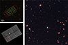 |
Fig. 1. Footprints of the HST and JWST images used in this work are shown in red and green, respectively, in the top-left panel. The bottom-left panel displays the stacked NIRCam/F322W2 image used in our analysis. The right panel shows a three-color composite image of the region marked with a red square in the bottom-left panel, where the blue, green, and red channels correspond to the stacked F606W, F814W, and F322W2 images, respectively. |
Summary of the HST and JWST imaging data used in this study.
Stellar photometry and astrometry were carried out using Jay Anderson’s KS2 software package, an advanced evolution of the ACS/WFC reduction code presented by Anderson et al. (2008). KS2 processes all exposures simultaneously and implements three complementary photometric strategies, each optimized for a different stellar brightness regime (e.g., Sabbi et al. 2016; Bellini et al. 2017; Milone et al. 2023).
Method I detects sources that produce a significant peak within a 5 × 5 pixel region after neighbor subtraction. For each star, KS2 measures flux and position in every exposure by fitting an effective point-spread function (ePSF; Anderson & King 2000) tailored to the star’s detector location. The sky background is estimated as an annulus spanning 4 to 8 pixels, and the final measurements are obtained by averaging results from all images.
Methods II and III are designed for stars too faint for robust PSF fitting. Both begin by subtracting neighboring stars and then derive fluxes from aperture photometry. Method II performs weighted aperture photometry in a 5 × 5 pixel box, reducing the contribution of pixels affected by crowding and adopting the same sky estimate as Method I.
Method III is optimized for very crowded regions and for faint stars with numerous exposures available. It uses a circular aperture of radius 0.75 pixels and determines the local background from an annulus between 2 and 4 pixels from the stellar position. KS2 also offers a suite of diagnostics to assess photometric quality. To ensure high-precision results, we retained only isolated stars that are well fitted by the ePSF model (see Sect. 2.4 in Milone et al. 2023).
The photometry was calibrated to the Vega magnitude system following the procedure described in Milone et al. (2023), using the appropriate encircled-energy corrections and zero points provided by STScI1. We account for pixel–area variations and corrected the coordinates for geometric distortion using the solutions of Anderson (2022) for ACS/WFC, and those provided by Jay Anderson for NIRCam data2. Finally, to derive the proper motions of stars in the field of view of Boötes I, we followed the procedure of Milone et al. (2023). In a nutshell, we first derived proper motions relative to the UFD by comparing the positions of stars at different epochs, integrating photometry from HST and JWST. By analyzing these proper motions, we distinguished the majority of Boötes I members from field stars. Stars with proper motions deviating more than three times the galaxy’s proper motion dispersion were excluded from the analysis presented in this paper (see Milone et al. 2023, for details).
We conducted artificial-star (AS) tests to estimate photometric errors and to generate the simulated CMD. Following the method outlined by Anderson et al. (2008), we created a list of 106 ASs. These ASs were designed to mimic the radial distribution and luminosity function of the observed stars and were placed along the fiducial line from the base of the RGB to the bottom of the MS.
To derive magnitudes and positions for the ASs, we employed the KS2 program, using the same procedures applied to the real stars. Our analysis focused exclusively on relatively isolated ASs that exhibited good PSF fits and satisfied the same selection criteria adopted for the real stars.
3. The color-magnitude diagram of Boötes I
Figure 2 shows the mF322W2 versus mF606W − mF322W2 CMD of Boötes I, together with the average error bars, derived from ASs. The CMD is predominantly populated by MS stars, which define a well-visible sequence that extends for approximately four F322W2 magnitudes below the turn-off (mF322W2 = 25.5 mag). A significant population of MS–MS binary systems is clearly visible on the red side of the MS, while the subgiant branch (SGB) and RGB are sparsely populated in the upper part of the diagram. There is no evidence of a large magnitude spread among SGB stars. The MS color broadening varies noticeably with magnitude: it is approximately 0.03 mag around the turn-off, increases to 0.08 mag at mF322W2 ∼ 23.3 mag, where it becomes comparable to that expected from observational uncertainties alone, and then suddenly increases for mF322W2 ≳ 24.0 mag.
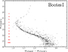 |
Fig. 2. mF322W2 vs. mF606W − mF322W2 CMD of Boötes I. The red bars indicate the average photometric errors. |
Section 4 exploits faint MS stars to constrain the metallicity distribution of stars in Boötes I, taking advantage of the fact that their color is strongly correlated with the chemical composition of this UFD. In Sect. 5, we take advantage of the narrow and well-defined upper MS to estimate the binary fraction.
4. Metallicity distribution
To better understand the CMD of Boötes I, in the left panel of Fig. 3 we compare the observed CMD with isochrones. The adopted metallicity values range from [Fe/H] = −3.4 to −1.553, whereas the corresponding values of [α/Fe] for each isochrone are derived from the relation between [α/Fe] and [Fe/H] inferred from Frebel et al. (2016, see their Fig. 8)
![Mathematical equation: $$ \begin{aligned}{[\alpha /\mathrm{Fe}]}= {\left\{ \begin{array}{ll} 0.35 \quad \mathrm{[Fe/H]} \le -2.5 \\ -0.31 \cdot \mathrm {[Fe/H]} - 0.43 \quad \mathrm{[Fe/H]} > -2.5 \\ \end{array}\right.}. \end{aligned} $$](/articles/aa/full_html/2026/04/aa58215-25/aa58215-25-eq2.gif) (1)
(1)
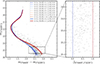 |
Fig. 3. mF322W2 vs. mF606W − mF322W2 CMD of Boötes I (left panel) and mF322W2 vs. ΔF606W, F322W2 verticalized diagram of the lower MS (right panel). We superimpose on the CMD nine isochrones with varying [Fe/H] and [α/Fe], as indicated in the inset. The isochrones used to verticalize the diagram are shown with continuous lines. |
The isochrones with [Fe/H] ≥ −3.2 are taken from the BaSTI database (Hidalgo et al. 2018)4, while those for more metal-poor populations were derived by linearly interpolating the colors and magnitudes between the [Fe/H] = −3.0 and −3.2 BaSTI isochrones. We obtained the best fit by using a distance modulus of (m − M)0 = 18.86, a foreground reddening of E(B − V) = 0.10 mag, and ages of 14–11 Gyr (see Appendix A for more details on the selection of ages).
Notably, these isochrones encompass the bulk of stars along the entire MS and indicate that the observed variation in MS width as a function of magnitude is consistent with stellar populations characterized by different metallicities. In particular, the isochrones indicate that the color spread of the lower MS (mF322W2 ≳ 24.4) is strongly driven by the chemical composition. Conversely, the color of the MS portion between mF322W2 ∼ 22.5 and 24.4 is much less sensitive to metallicity changes, since the isochrones shown in Fig. 3 exhibit reduced color separation and even overlap within this magnitude range.
To investigate the metallicity distribution of Boötes I stars, we selected MS stars within the CMD region defined by 24.5 < mF322W2 < 25.5 mag, where stellar colors are strongly affected by metallicity. Following the procedure described in Milone et al. (2017), we verticalized the selected stars such that the isochrones with [Fe/H] = −3.2 and [Fe/H] = −1.7 (solid blue and red lines in Fig. 3) are mapped onto vertical lines with abscissae equal to 0 and 1, respectively. For each star, we computed the pseudo-color parameter
 (2)
(2)
where X represents the color of a star in the CMD.
The resulting verticalized diagram is shown in the right panel of Fig. 3. The parameter ΔF606W, F322W2 serves as a proxy for the metallicity distribution. Figure 4 displays the kernel (ϕ), evaluated using a Gaussian kernel with a bandwidth of 0.1, and the cumulative (ρ) distributions of ΔF606W, F322W2 as solid black lines. These distributions are approximately symmetric, and the majority of MS stars exhibit intermediate values of ΔF606W, F322W2.
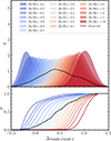 |
Fig. 4. Kernel (top) and cumulative (bottom) distributions of ΔF606W, F322W2 for faint MS stars. The black curves are derived from the observed Boötes I members, while the colored curves are obtained from the simulated CMDs. |
To gather information on metallicity, we compared the observed photometry with simulated diagrams. We used ASs to generate seventeen simulated CMDs corresponding to simple stellar populations with metallicities ranging from [Fe/H] = −3.2 to −1.7 in steps of 0.1 dex, assuming the relation between [α/Fe] and [Fe/H] (Eq. (1)) inferred from Frebel et al. (2016). In addition, we produced two limiting simulated CMDs corresponding to stellar populations with [Fe/H] = −3.4 and −1.55. A binary fraction of 0.30 was adopted, with a flat mass-ratio distribution. The input colors and magnitudes of the ASs were obtained from the BaSTI isochrones. We derived the ΔF606W, F322W2 pseudo-color for stars in each simulated diagram by applying the same methodology and adopting the same magnitude range as for the observed stars. In Fig. 4, we compare the kernel-density and cumulative distributions of the observed stars (black lines) with those derived from the simulated CMDs.
To estimate the metallicity distribution of Boötes I, we adapted the sample of MS stars identified in Fig. 3 to the method introduced by Stauffer (1980) and widely adopted for studying stellar populations (e.g., Cignoni & Tosi 2010; Cordoni et al. 2022; Legnardi et al. 2022). In essence, we compared the cumulative ΔF606W, F322W2 distribution of a large number of simulated stellar populations with the observed one.
We constructed a composite simulated population by summing the individual model populations, assigning to each population j a weighting factor cj that defines its fractional contribution to the total number of stars in the resulting ΔF606W, F322W2 cumulative distribution. The coefficient cj ranges from 0 to 1. The composite cumulative distribution was then quantitatively compared with the observed distribution using a classical χ2 minimization procedure. This optimization was performed using the open-source pyGAD package5, which provides the array of coefficients cj describing the relative contribution of each model population to the best-fitting cumulative distribution of the Boötes I stars.
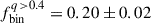
The bottom-left panel of Fig. 5 compares the observed cumulative distribution with the best-fit model. For completeness, the upper-left panel of the same figure shows the comparison between the observed kernel-density distribution and that derived from the best-fit simulation. As shown in Table 3, the best fitting simulated distribution gives a mean iron abundance of [Fe/H] = −2.53 ± 0.05 and a dispersion of 0.41 ± 0.03 dex. These values are consistent with spectroscopic measurements, [Fe/H] = −2.60 ± 0.03 dex, with a metallicity dispersion of 0.34 ± 0.03 dex (Longeard et al. 2022).
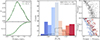 |
Fig. 5. Left: comparison between the observed (black) and best-fit simulated (green) kernel (top) and cumulative (bottom) distributions of ΔF606W, F322W2. Middle: [Fe/H] histogram that best reproduces the observations of Boötes I. The dashed black and gray distributions are from a spectroscopic survey from Jenkins et al. (2021) and Longeard et al. (2022), respectively. Right: comparison between the observed (top) and simulated (bottom) CMDs, zoomed in on the MS region used to infer the metallicity distribution. The colors of the simulated stars indicate their iron abundance, as shown in the middle panel. |
Binary fraction with mass ratio larger than 0.4, total binary fraction, slope of the mass ratio distribution, average iron abundance, and dispersion of Boötes I.
The corresponding metallicity histogram is shown in the middle panel of Fig. 5, revealing a main peak close to the average metallicity value. The most metal-poor stars have [Fe/H] ∼ −3.4, and their number gradually increases up to the maximum around the mean metallicity. The number of stars then decreases toward higher metallicities, with a tail of stars having [Fe/H] ≳ −2. In particular, we found that the majority of stars ∼85% have [Fe/H] < −2, and that roughly ∼17% have [Fe/H] < −3. Finally, the right panels of Fig. 5 compare the observed (top) and simulated (bottom) CMDs, zoomed in on the faint end of the MS, highlighting the strong similarity between the two diagrams.
To assess the impact of the adopted [α/Fe] distribution, we re-derived stellar metallicities assuming two extreme and constant values, [α/Fe] = 0.35 and [α/Fe] = 0.00 dex. Although neither of these simplified prescriptions accurately reproduces the observed [α/Fe] distribution in Boötes I, they provide a useful way to quantify the sensitivity of our results to this assumption. For [α/Fe] = 0.35, the inferred metallicity distribution closely resembles the reference distribution derived in this work, but is shifted toward slightly lower metallicities, with a mean [Fe/H]= − 2.60 ± 0.02 and a dispersion of ∼0.3 dex. In contrast, adopting a solar-scaled composition ([α/Fe] = 0.00) leads to a substantial shift of the metallicity distribution toward higher values, yielding a mean [Fe/H]= − 2.10 ± 0.02 and a comparable dispersion of ∼0.3 dex. This result is in clear disagreement with both our fiducial metallicity distribution and those obtained from spectroscopic studies (Norris et al. 2010b; Koposov et al. 2011; Gilmore et al. 2013; Ishigaki et al. 2014; Jenkins et al. 2021; Longeard et al. 2022; Sandford et al. 2025). Such a discrepancy is expected since assuming solar-scaled abundances for all stars is inconsistent with the enhanced [α/Fe] ratios observed in Boötes I.
5. The binary map
To investigate the population of binaries along the MS of Boötes I, we introduce the “binary map”, a new diagnostic tool analogous to the chromosome map6 of GCs, designed to distinguish binaries with different mass ratios. This diagram is based on the well-known photometric properties of unresolved binary systems composed of two MS stars, which appear as single point-like sources with a total magnitude
 (3)
(3)
where m1 is the magnitude of the primary (brightest) star and F1 and F2 are the fluxes of the primary and secondary components, respectively. In a simple stellar population, the flux of MS stars depends on their mass following a specific mass-luminosity relation. As a consequence, the total magnitude of a binary system composed of two MS stars can be uniquely determined by the mass of the primary component and the mass ratio, q = M2/M1, where M1 and M2 are the masses of the primary and secondary stars.
To construct the binary map, we used the setup illustrated in Fig. 6, where the shaded area superimposed on the CMD of Boötes I highlights the region, hereafter referred to as region A, used to study binary systems. This region includes single stars with 22.5 < mF322W2 < 24.5 and binary systems whose primary component falls within the same magnitude interval. We selected this portion of the CMD because of the partial overlap between isochrones of different metallicities (Fig. 3), so that binaries are well separated from single stars.
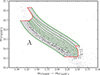 |
Fig. 6. mF322W2 vs. mF606W − mF322W2 CMD of Boötes I, where the gray shaded area indicates the region used to study binaries and derive the binary map. The nine green lines delimit the eight subregions (R1 − R8) adopted for the binary analysis. The bluest line represents the fiducial sequence of single stars, shifted to the blue to encompass the bulk of MS stars, while the reddest line corresponds to the fiducial of equal-mass binaries, shifted to the red to include most binaries. The remaining lines represent fiducial sequences of binaries with mass ratios ranging from 0.3 to 1.0, as indicated. |
As shown in Fig. 6, we defined nine green reference lines, hereafter referred to as lines 1–9. Line 1, which represents the left boundary of region A, corresponds to the fiducial line of Boötes I shifted toward the blue by three times the average color error (∼0.16 mag) to enclose the bulk of MS stars. Lines 2 to 8, the dashed ones, correspond to the fiducial sequences of binary systems with mass ratios q = 0.3, 0.4, 0.5, 0.6, 0.7, 0.8, and 1.0, respectively.
These fiducial lines were derived following the same procedure as adopted in our previous works (e.g., Milone et al. 2012; Muratore et al. 2024), using the MS fiducial line and the mass–luminosity relation provided by the best-fit isochrone to compute the colors and magnitudes corresponding to binaries with different q values. Finally, line 9 represents the fiducial sequence of equal-mass binaries shifted toward the red by two times the average color error (∼0.11 mag), to include binaries with large mass ratios that appear redder due to observational uncertainties. These nine lines define eight regions, namely R1–R8. The region R1 includes the bulk of single stars and binaries with a mass ratio smaller than 0.3. The regions R2–R7 contain binaries in successive 0.1-wide q bins from 0.3 to 0.8, while the region R8 covers 0.8 ≤ q ≤ 1.0 (width 0.2). Region 8 mostly hosts binaries that are shifted to the red by photometric uncertainties.
We applied a two-step verticalization of the diagram following the procedure used to derive the chromosome maps of GCs. In the first step, we normalize the colors so that lines 1–9 are transformed into vertical lines. To achieve this, we adapt Eq. (1) from Milone et al. (2025) to each region (Ri, i = 1–8) and derived the quantities
 (4)
(4)
where X = mF606W − mF322W2, and Wi is the color separation between lines i + 1 and i, measured at mF322W2 = 23.5 mag. We then combined these quantities to define the pseudo-color
 (5)
(5)
In the second step, verticalization is performed in magnitude. Specifically, for each region, we define the quantity
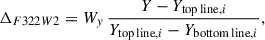 (6)
(6)
where Y = mF322W2, and Wy denotes the magnitude interval of region R1. The top line corresponds to the red top line from mF322W2 = 22.5 in region R1, to the segment with mF322W2 = 22.5 − 0.75 in region R8, tracing binaries whose primary star has mF322W2 = 22.5 and mass ratios between 0.3 and 1.0 in the remaining regions. The red bottom line is defined analogously, but for mF322W2 = 24.4.
The resulting ΔF322W2 versus  binary map is shown in the left panel of Fig. 7, together with the ΔF606W, F322W2 histogram. The majority of stars lie within the region 1–2, but a well-populated tail extends into regions 3–8, confirming that Boötes I hosts a significant fraction of binaries with q > 0.4.
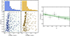 |
Fig. 7. Binary maps and mass-ratio distribution for Boötes I. Left: Observed binary map (in blue), with the corresponding ΔF606W, F322W2 distribution shown in the top panel. The vertical dashed lines indicate the nine reference loci used to construct the map, including the fiducial sequences of binary systems with different mass ratios, q, whose values are labeled in the figure. Middle: Best-fit binary map (in gold). Right: Mass-ratio distribution derived from the best fit; the green line and shaded region indicate the linear fit and its associated uncertainty. |
5.1. The fraction of binaries in Boötes I
To reproduce the observed stellar distribution across the binary map, we adopted an iterative procedure based on ASs. The purpose of this method is to generate a simulated sample whose recovered stars reproduce, region by region, the number of observed stars Ni.
In the first iteration, for each region, we generated a number of input ASs equal to half of the observed count, that is,

Each AS was assigned input magnitudes and colors that placed it within the region boundaries. Due to observational uncertainties and photometric scatter, some ASs injected within a given region were later recovered in different regions of the binary map. The number of ASs actually recovered in each bin after this first iteration is denoted by nGEN, i, 1.
In the second iteration, we injected an additional set of ASs. The number of newly added stars in each bin was determined as
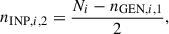
so as to gradually compensate for bins where the number of recovered stars was smaller than the observed value. The cumulative number of injected stars in each bin after this step is therefore

Once again, we measured the number of ASs recovered in each bin, nOBS, i, 2, after running the full reduction and selection procedure.
The process was repeated iteratively, changing the number of injected stars in each bin according to the residual difference between the observed and recovered counts. Convergence was reached when, for all bins,
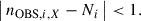
This iterative approach ensures that the AS sample reproduces the observed distribution of stars across the binary map while accounting for photometric scatter and completeness effects.
Figure 7 compares the observed binary map of Boötes I (left) with the best fit simulated one (middle). The corresponding  histogram distributions are shown in the top panels. This procedure provides the numbers of single stars and binaries with their respective mass ratios.
The right panel of Fig. 7 illustrates the binary frequency, defined as the fraction of binaries in five intervals of mass ratio divided by the width of each interval, as a function of the mass ratio. The best-fit straight line has a slope of −0.30 ± 0.15, which is consistent with a flat distribution at the 2σ level. We consider only binaries with mass ratios larger than 0.4 because the small color separation makes it challenging to robustly distinguish low mass ratio binaries from single stars. We obtained an almost flat mass ratio distribution, consistent with the results of Raghavan et al. (2010) and Milone et al. (2012) for solar-type stars in the Galactic field and for 29 GCs, respectively.
By combining the results of the five bins, we derived a binary fraction with a mass ratio greater than 0.4 of  . Assuming this mass-ratio distribution, we infer an overall binary fraction of
  , taking into account a minimum mass of 0.075 M⊙ for the secondary star. The derived parameters are summarized in Table 3. Figure 8 shows a comparison between observed Boötes I and simulated CMDs with the derived binary fraction, metallicity distribution, and ages of 11–14 Gyr.
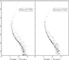 |
Fig. 8. Comparison of the observed (left) and simulated (right) CMD of Boötes I. |
5.2. Comparison with UFDs, clusters, and field stars
The binary fraction we measure in Boötes I is consistent with the spectroscopic estimate of ∼0.28 reported by Gennaro et al. (2018). It is also similar to the values found in Leo II and in the inner region of Ursa Minor, which are ∼0.30 and ∼0.33, respectively (Spencer et al. 2017; Qiu et al. 2025). Moreover, the binary fraction of Boötes I is comparable to that typically observed in Galactic open clusters (Cordoni et al. 2023), and in Magellanic Cloud clusters (Mohandasan et al. 2024), and significantly higher than that found in most GCs (Milone et al. 2012, 2016). This comparison is illustrated in the left and central panels of Fig. 9. The left panel shows the anticorrelation between the binary fraction in GCs (Milone et al. 2012, 2016) and the mass of the host cluster (Baumgardt et al. 2020). Remarkably, when considering only the stellar mass (Jenkins et al. 2021), Boötes I exhibits a binary fraction similar to that of GCs with comparable masses. In contrast, when the dynamical mass (Martin et al. 2008) is adopted, Boötes I deviates from the relation followed by the bulk of GCs.
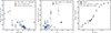 |
Fig. 9. Comparison between Boötes I, Galactic GCs, and field stars. Left: fraction of binaries with mass ratio q > 0.5 in the cores of GCs (Milone et al. 2012, 2016), compared with that in Boötes I. The red and yellow diamonds represent Boötes I, corresponding to the dynamical and stellar masses, respectively, from Martin et al. (2008) and Jenkins et al. (2021). GC masses are adopted from Baumgardt et al. (2020). Middle: binary fraction plotted against the concentration parameter, rh/rt. Radii are taken from the 2010 edition of the Harris (1996) catalog for GCs, and from Okamoto et al. (2012) and Belokurov et al. (2006) for Boötes I. Right: total binary fraction as a function of the primary-component mass. Gray dots correspond to Galactic field stars compiled in the review by Offner et al. (2023), and the green diamond indicates the binary fraction measured for the SMC field by Legnardi et al. (2025). |
For completeness, the middle panel of Fig. 9 shows the relation between the binary fraction and the concentration parameter, defined as the ratio between the half-light radius and the tidal radius of the stellar system. The concentration parameter is often used to distinguish GCs from UFDs. We adopted GC structural parameters from the 2010 edition of the Harris (1996) catalog, and those for Boötes I from Okamoto et al. (2012) and Koposov et al. (2011). As expected, Boötes I exhibits a larger rh/rt ratio than that typically observed in GCs. There is no clear evidence for a strong correlation between concentration and binary fraction, although stellar systems (both Boötes I and GCs) with rh/rt ≳ 0.15 tend to have, on average, higher binary fractions than the remaining GCs. Nevertheless, the large scatter in the binary fraction among systems with similar values of rh/rt prevents us from drawing firm conclusions about any relation between concentration and binary fraction. Finally, as shown in the right panel of Fig. 9, where we plot the binary fraction against the mass of the primary stars, Boötes I follows the same trend defined by the Milky Way and Small Magellanic Cloud field stars (Offner et al. 2023; Legnardi et al. 2025).
6. Summary and discussion
We derived high-precision HST and JWST photometry for stars in the core of the UFD galaxy Boötes I, using the F606W band of ACS/WFC and the F322W2 band of NIRCam. The resulting exquisite CMD reveals a remarkably narrow and bright MS, where the observed color spread is comparable to that expected from photometric uncertainties alone in the F322W2 magnitude range ∼22.5–24.5. However, at fainter magnitudes, the MS color broadening increases sharply, reaching ∼0.4 mag around mF322W2 ∼ 25.0. Significant color broadening is also evident near the MS turnoff, which transitions into a narrow and sparsely populated SGB. Comparison with isochrones indicates that this behavior is consistent with the presence of stellar populations spanning a range of metallicities. Notably, the CMD also displays a prominent binary sequence, formed by pairs of MS stars, located on the red side of the single-star MS. We used these data to infer the metallicity distribution and to investigate the population of binaries.
-
The wide color broadening of stars fainter than mF322W2 ∼ 24 provides an opportunity to constrain the chemical composition of stars in Boötes I. After accounting for the [α/Fe]–[Fe/H] relation inferred from high-resolution spectroscopy (Frebel et al. 2016), the color distribution of faint stars allows for an accurate determination of the metallicity distribution (see also, Legnardi et al. 2022, 2024, for similar determinations in GCs). Based on a sample of 265 stars, we infer an average iron abundance of [Fe/H]= − 2.53 ± 0.05, with a dispersion of 0.41 ± 0.03. The metallicity distribution spans a wide range, from [Fe/H] ∼ −3.4 to [Fe/H]∼ − 1.55, indicating that approximately ∼85% have [Fe/H]< − 2, and that roughly ∼17% have [Fe/H] < −3. These findings are consistent and confirm previous high-resolution spectroscopic studies based on smaller samples of RGB stars (Jenkins et al. 2021; Longeard et al. 2022; Sandford et al. 2025). This approach, applied here for the first time to a UFD, combines photometric and spectroscopic information ([α/Fe]-[Fe/H] relation) to analyze a large sample of MS stars. Our analysis showed that this new technique can be used for systems where only a limited number of spectra are available, as well as for fainter systems, including the increasing population of ambiguous ultra-faint objects that elude spectroscopic observation because they contain almost no red giant branch stars.
-
We take advantage of the high-quality CMD, where the binary sequence is visible with unprecedented clarity, to infer the fraction of binary systems composed of MS stars. To this end, we introduced a new pseudo-CMD, which we dubbed binary map, in which the pseudo-color serves as an indicator of the mass ratio. From this analysis, we derived a binary fraction of
 for systems with a mass ratio q > 0.4, and inferred an approximately flat mass ratio distribution with a slope of −0.30 ± 0.15. By assuming a flat mass ratio distribution, we extrapolated a total binary fraction of 0.30 ± 0.03, comparable to what was inferred by Gennaro et al. (2018) to characterize the initial mass function of Boötes I using ACS/WFC data (∼0.28), and to what was derived in Leo II (∼0.30) and in the inner region of Ursa Minor (∼0.33) (Spencer et al. 2017; Qiu et al. 2025). The binary fraction is a crucial parameter for constraining the dynamical mass of UFDs, and hence their dark matter content. Indeed, in UFDs, which exhibit relatively small velocity dispersions (e.g., Simon & Geha 2007), the contribution from binary stars can reach a few km s−1, comparable to the dispersions observed in these ancient stellar systems (e.g., Spencer et al. 2018; Pianta et al. 2022). A relatively large binary fraction of ∼30%, as derived for Boötes I, can artificially broaden the measured velocity distribution and thus lead to an incorrect estimate of the dark matter content, as recently demonstrated by studies based on the analytic method (Gration et al. 2025). The binary fraction observed in Boötes I is comparable to that typically found in stellar systems with similar stellar mass, such as Galactic and Magellanic Cloud open clusters (Cordoni et al. 2023; Mohandasan et al. 2024), as well as in the Galactic and Small Magellanic Cloud field for stars of similar masses (Offner et al. 2023; Legnardi et al. 2025). Compared with GCs, Boötes I follows the well-known anticorrelation between the binary fraction and the mass of the host stellar system. Using the stellar mass (Martin et al. 2008), the dwarf galaxy aligns remarkably well with this relation; however, this agreement breaks down when the dynamical mass is considered (Jenkins et al. 2021). Although caution must be exercised when comparing GCs and UFDs, given their different structural properties and evolutionary histories, the fact that Boötes I follows the GC trend indicates that dark matter, consistent with its collisionless nature, shapes the global gravitational potential but does not engage in local dynamical interactions that would alter binary fractions, a result that agrees with the simulation run by Livernois et al. (2023), who found that close binaries, as analyzed here, were not affected by the presence of dark matter.
Data availability
Photometry is available at the CDS via https://cdsarc.cds.unistra.fr/viz-bin/cat/J/A+A/708/A100
Acknowledgments
We would like to thank the anonymous referee for helpful comments that significantly improved the quality of the paper. This work has been funded by the European Union – NextGenerationEU RRF M4C2 1.1 (PRIN 2022 2022MMEB9W: “Understanding the formation of globular clusters with their multiple stellar generations”, CUP C53D23001200006), and from the European Union’s Horizon 2020 research and innovation programme under the Marie Skłodowska-Curie Grant Agreement No. 101034319 and from the European Union – NextGenerationEU (beneficiary: T. Ziliotto). This research is based on observations made with the NASA/ESA Hubble Space Telescope obtained from the Space Telescope Science Institute, which is operated by the Association of Universities for Research in Astronomy, Inc., under NASA contract NAS 5–26555. These observations are associated with programs 12549,15317. This work is based [in part] on observations made with the NASA/ESA/CSA James Webb Space Telescope. The data were obtained from the Mikulski Archive for Space Telescopes at the Space Telescope Science Institute, which is operated by the Association of Universities for Research in Astronomy, Inc., under NASA contract NAS 5-03127 for JWST. These observations are associated with program 3849.
References
- Anderson, J. 2022, One-Pass HST Photometry with hst1pass, Instrument Science Report WFC3 2022–5, 55 [Google Scholar]
- Anderson, J., & King, I. R. 2000, PASP, 112, 1360 [NASA ADS] [CrossRef] [Google Scholar]
- Anderson, J., Sarajedini, A., Bedin, L. R., et al. 2008, AJ, 135, 2055 [Google Scholar]
- Battaglia, G., & Nipoti, C. 2022, Nat. Astron., 6, 1492 [NASA ADS] [CrossRef] [Google Scholar]
- Baumgardt, H., Sollima, A., & Hilker, M. 2020, PASA, 37, e046 [Google Scholar]
- Bellini, A., Anderson, J., Bedin, L. R., et al. 2017, ApJ, 842, 6 [NASA ADS] [CrossRef] [Google Scholar]
- Belokurov, V., Zucker, D. B., Evans, N. W., et al. 2006, ApJ, 647, L111 [NASA ADS] [CrossRef] [Google Scholar]
- Belokurov, V., Walker, M. G., Evans, N. W., et al. 2010, ApJ, 712, L103 [NASA ADS] [CrossRef] [Google Scholar]
- Brown, T. M., Tumlinson, J., Geha, M., et al. 2014, ApJ, 796, 91 [NASA ADS] [CrossRef] [Google Scholar]
- Cignoni, M., & Tosi, M. 2010, Adv. Astron., 2010, 158568 [CrossRef] [Google Scholar]
- Cordoni, G., Milone, A. P., Marino, A. F., et al. 2022, Nat. Commun., 13, 4325 [NASA ADS] [CrossRef] [Google Scholar]
- Cordoni, G., Milone, A. P., Marino, A. F., et al. 2023, A&A, 672, A29 [NASA ADS] [CrossRef] [EDP Sciences] [Google Scholar]
- Durbin, M. J., Choi, Y., Savino, A., et al. 2025, ApJ, 992, 106 [Google Scholar]
- Ford, H. C., Clampin, M., Hartig, G. F., et al. 2003, SPIE Conf. Ser., 4854, 81 [NASA ADS] [Google Scholar]
- Frebel, A., Norris, J. E., Gilmore, G., & Wyse, R. F. G. 2016, ApJ, 826, 110 [NASA ADS] [CrossRef] [Google Scholar]
- Gennaro, M., Tchernyshyov, K., Brown, T. M., et al. 2018, ApJ, 855, 20 [NASA ADS] [CrossRef] [Google Scholar]
- Gilmore, G., Norris, J. E., Monaco, L., et al. 2013, ApJ, 763, 61 [NASA ADS] [CrossRef] [Google Scholar]
- Gration, A., Hendriks, D. D., Das, P., Heber, D., & Izzard, R. G. 2025, MNRAS, 543, 1120 [Google Scholar]
- Harris, W. E. 1996, AJ, 112, 1487 [Google Scholar]
- Hidalgo, S. L., Pietrinferni, A., Cassisi, S., et al. 2018, ApJ, 856, 125 [Google Scholar]
- Ishigaki, M. N., Aoki, W., Arimoto, N., & Okamoto, S. 2014, A&A, 562, A146 [NASA ADS] [CrossRef] [EDP Sciences] [Google Scholar]
- Jenkins, S. A., Li, T. S., Pace, A. B., et al. 2021, ApJ, 920, 92 [NASA ADS] [CrossRef] [Google Scholar]
- Kim, D., Jerjen, H., Mackey, D., Da Costa, G. S., & Milone, A. P. 2015, ApJ, 804, L44 [NASA ADS] [CrossRef] [Google Scholar]
- Kirby, E. N., Guhathakurta, P., & Sneden, C. 2008, ApJ, 682, 1217 [Google Scholar]
- Koposov, S. E., Gilmore, G., Walker, M. G., et al. 2011, ApJ, 736, 146 [NASA ADS] [CrossRef] [Google Scholar]
- Lai, D. K., Lee, Y. S., Bolte, M., et al. 2011, ApJ, 738, 51 [CrossRef] [Google Scholar]
- Legnardi, M. V., Milone, A. P., Armillotta, L., et al. 2022, MNRAS, 513, 735 [NASA ADS] [CrossRef] [Google Scholar]
- Legnardi, M. V., Milone, A. P., Cordoni, G., et al. 2024, A&A, 687, A160 [NASA ADS] [CrossRef] [EDP Sciences] [Google Scholar]
- Legnardi, M. V., Muratore, F., Milone, A. P., et al. 2025, A&A, 702, A180 [NASA ADS] [CrossRef] [EDP Sciences] [Google Scholar]
- Livernois, A. R., Vesperini, E., & Pavlík, V. 2023, MNRAS, 521, 4395 [NASA ADS] [CrossRef] [Google Scholar]
- Longeard, N., Jablonka, P., Arentsen, A., et al. 2022, MNRAS, 516, 2348 [NASA ADS] [CrossRef] [Google Scholar]
- Marino, A. F., Milone, A. P., Karakas, A. I., et al. 2015, MNRAS, 450, 815 [NASA ADS] [CrossRef] [Google Scholar]
- Martin, N. F., de Jong, J. T. A., & Rix, H.-W. 2008, ApJ, 684, 1075 [NASA ADS] [CrossRef] [Google Scholar]
- McConnachie, A. W. 2012, AJ, 144, 4 [Google Scholar]
- McConnachie, A. W., & Côté, P. 2010, ApJ, 722, L209 [NASA ADS] [CrossRef] [Google Scholar]
- Milone, A. P., Piotto, G., Bedin, L. R., et al. 2012, A&A, 540, A16 [NASA ADS] [CrossRef] [EDP Sciences] [Google Scholar]
- Milone, A. P., Marino, A. F., Piotto, G., et al. 2015, ApJ, 808, 51 [NASA ADS] [CrossRef] [Google Scholar]
- Milone, A. P., Marino, A. F., Bedin, L. R., et al. 2016, MNRAS, 455, 3009 [CrossRef] [Google Scholar]
- Milone, A. P., Piotto, G., Renzini, A., et al. 2017, MNRAS, 464, 3636 [Google Scholar]
- Milone, A. P., Cordoni, G., Marino, A. F., et al. 2023, A&A, 672, A161 [NASA ADS] [CrossRef] [EDP Sciences] [Google Scholar]
- Milone, A. P., Marino, A. F., Bernizzoni, M., et al. 2025, A&A, 698, A247 [NASA ADS] [CrossRef] [EDP Sciences] [Google Scholar]
- Mohandasan, A., Milone, A. P., Cordoni, G., et al. 2024, A&A, 681, A42 [NASA ADS] [CrossRef] [EDP Sciences] [Google Scholar]
- Muratore, F., Milone, A. P., D’Antona, F., et al. 2024, A&A, 692, A135 [NASA ADS] [CrossRef] [EDP Sciences] [Google Scholar]
- Norris, J. E., Gilmore, G., Wyse, R. F. G., et al. 2008, ApJ, 689, L113 [Google Scholar]
- Norris, J. E., Wyse, R. F. G., Gilmore, G., et al. 2010a, ApJ, 723, 1632 [NASA ADS] [CrossRef] [Google Scholar]
- Norris, J. E., Yong, D., Gilmore, G., & Wyse, R. F. G. 2010b, ApJ, 711, 350 [NASA ADS] [CrossRef] [Google Scholar]
- Offner, S. S. R., Moe, M., Kratter, K. M., et al. 2023, ASP Conf. Ser., 534, 275 [NASA ADS] [Google Scholar]
- Okamoto, S., Arimoto, N., Yamada, Y., & Onodera, M. 2012, ApJ, 744, 96 [NASA ADS] [CrossRef] [Google Scholar]
- Pianta, C., Capuzzo-Dolcetta, R., & Carraro, G. 2022, ApJ, 939, 3 [NASA ADS] [CrossRef] [Google Scholar]
- Qiu, T., Wang, W., Koposov, S., et al. 2025, ArXiv e-prints [arXiv:2512.04477] [Google Scholar]
- Raghavan, D., McAlister, H. A., Henry, T. J., et al. 2010, ApJS, 190, 1 [Google Scholar]
- Rieke, M. J., Kelly, D. M., Misselt, K., et al. 2023, PASP, 135, 028001 [CrossRef] [Google Scholar]
- Sabbi, E., Lennon, D. J., Anderson, J., et al. 2016, ApJS, 222, 11 [NASA ADS] [CrossRef] [Google Scholar]
- Sacchi, E., Richstein, H., Kallivayalil, N., et al. 2021, ApJ, 920, L19 [NASA ADS] [CrossRef] [Google Scholar]
- Sandford, N. R., Li, T. S., Koposov, S. E., et al. 2025, ArXiv e-prints [arXiv:2509.02546] [Google Scholar]
- Savino, A., Weisz, D. R., Skillman, E. D., et al. 2023, ApJ, 956, 86 [Google Scholar]
- Simon, J. D. 2019, ARA&A, 57, 375 [NASA ADS] [CrossRef] [Google Scholar]
- Simon, J. D., & Geha, M. 2007, ApJ, 670, 313 [NASA ADS] [CrossRef] [Google Scholar]
- Spencer, M. E., Mateo, M., Walker, M. G., et al. 2017, AJ, 153, 254 [NASA ADS] [CrossRef] [Google Scholar]
- Spencer, M. E., Mateo, M., Olszewski, E. W., et al. 2018, AJ, 156, 257 [NASA ADS] [CrossRef] [Google Scholar]
- Stauffer, J. R. 1980, AJ, 85, 1341 [Google Scholar]
- Willman, B., Geha, M., Strader, J., et al. 2011, AJ, 142, 128 [NASA ADS] [CrossRef] [Google Scholar]
- Zoutendijk, S. L., Brinchmann, J., Bouché, N. F., et al. 2021, A&A, 651, A80 [NASA ADS] [CrossRef] [EDP Sciences] [Google Scholar]
STScI calibration resources are available at: ACS: https://www.stsci.edu/hst/instrumentation/acs/data-analysis/zeropoints; NIRCam: https://jwst-docs.stsci.edu/jwst-near-infrared-camera/nircam-performance/nircam-absolute-flux-calibration-and-zeropoints#gsc.tab=0.
In selecting the metallicity interval for the isochrone, the lower limit was set by the unavailability of isochrones at very low metallicities, while the onset of the binary region constrained the upper limit. To exclude most binary stars, we therefore restricted our analysis to metallicities below −1.55.
We used pyGAD (https://pygad.readthedocs.io/), a genetic algorithm Python library that reduces the likelihood of convergence to a local rather than a global minimum. The coefficients were normalized using a softmax function, ensuring that their sum equals unity and can be interpreted as fractional contributions resulting from the minimization.
The chromosome map (Milone et al. 2015, 2017) is a powerful diagnostic tool for studying stellar populations in GCs. It is a pseudo–two-color diagram that is highly sensitive to the chemical differences between distinct stellar populations.
Appendix A: On the age of Boötes I
A visual inspection of the CMD shown in Fig. 2 reveals that the sparsely populated SGB of Boötes I appears remarkably narrow and well defined. Since the SGB is highly sensitive to stellar age, in this Appendix we examine whether the current dataset allows us to place meaningful constraints on the ages of the stellar populations in Boötes I. In addition, we assess how the choice of isochrone ages adopted throughout this paper affects the derived binary fractions and the inferred metallicity distribution.
The left panels of Fig. A.1 reproduce the CMD shown in Fig. 2, zoomed in around the SGB region, with two BaSTI isochrones overplotted, corresponding to the extreme metallicity values ([Fe/H]=−3.2 and −1.7). The bottom panel displays the isochrones with different ages (14 and 11 Gyr), introduced in Sect.,4, and adopted in this work.
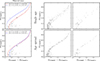 |
Fig. A.1. mF322W2 vs. mF606W − mF322W2 CMDs zoomed in around the SGB. The left panels show the observed CMDs of Boötes I, where the red and blue lines are isochrones with different [Fe/H], [α/Fe], and ages, as indicated in the insets. The middle panels show simulated CMDs composed of coeval stellar populations (top) and of stellar populations with different ages (bottom). The right panels are the same as the middle panels, but include approximately the same number of stars as in the observed CMDs. |
These two isochrones nearly overlap along the SGB. The top panel, instead, shows isochrones of the same age (13 Gyr), which are widely separated in color along the SGB.
The middle panels of Fig. A.1 present two simulated CMDs. In both cases, we adopted the same luminosity function and binary fraction as in the observed CMD, but with a total number of stars increased by a factor of ten to reduce statistical noise. We also assumed the same metallicity distribution inferred in this study. The two simulated CMDs differ only in the age distribution of stellar populations with different metallicities. The bottom-middle panel corresponds to the age distribution adopted in Sect.,4, whereas the top-middle panel assumes all populations are coeval. The right panels show the same simulated CMDs as in the middle panels, but rescaled to match the number of stars in the observed CMD.
Although the observed stars are distributed along a relatively narrow SGB—suggesting, at first glance, a prolonged star formation—the limited number of SGB stars prevents us from drawing firm conclusions about the ages of the Boötes I stellar populations. However, this hint of a prolonged star formation is in agreement with what was found by Brown et al. (2014) and Durbin et al. (2025), who inferred a primary star formation event about 13.4 Gyr ago, followed by residual star formation persisting until roughly 11 Gyr ago.
To assess the robustness of our results on the binary fraction and metallicity distribution, we repeated the analyses presented in Sects. 4 and 5 using coeval isochrones. We verified that the results remain unchanged. This outcome is expected, since the determination of the binary fraction and metallicity distribution is based on MS stars, whose position in the CMD is largely insensitive to age.
All Tables
Binary fraction with mass ratio larger than 0.4, total binary fraction, slope of the mass ratio distribution, average iron abundance, and dispersion of Boötes I.
All Figures
|
Fig. 1. Footprints of the HST and JWST images used in this work are shown in red and green, respectively, in the top-left panel. The bottom-left panel displays the stacked NIRCam/F322W2 image used in our analysis. The right panel shows a three-color composite image of the region marked with a red square in the bottom-left panel, where the blue, green, and red channels correspond to the stacked F606W, F814W, and F322W2 images, respectively. |
| In the text | |
|
Fig. 2. mF322W2 vs. mF606W − mF322W2 CMD of Boötes I. The red bars indicate the average photometric errors. |
| In the text | |
|
Fig. 3. mF322W2 vs. mF606W − mF322W2 CMD of Boötes I (left panel) and mF322W2 vs. ΔF606W, F322W2 verticalized diagram of the lower MS (right panel). We superimpose on the CMD nine isochrones with varying [Fe/H] and [α/Fe], as indicated in the inset. The isochrones used to verticalize the diagram are shown with continuous lines. |
| In the text | |
|
Fig. 4. Kernel (top) and cumulative (bottom) distributions of ΔF606W, F322W2 for faint MS stars. The black curves are derived from the observed Boötes I members, while the colored curves are obtained from the simulated CMDs. |
| In the text | |
|
Fig. 5. Left: comparison between the observed (black) and best-fit simulated (green) kernel (top) and cumulative (bottom) distributions of ΔF606W, F322W2. Middle: [Fe/H] histogram that best reproduces the observations of Boötes I. The dashed black and gray distributions are from a spectroscopic survey from Jenkins et al. (2021) and Longeard et al. (2022), respectively. Right: comparison between the observed (top) and simulated (bottom) CMDs, zoomed in on the MS region used to infer the metallicity distribution. The colors of the simulated stars indicate their iron abundance, as shown in the middle panel. |
| In the text | |
|
Fig. 6. mF322W2 vs. mF606W − mF322W2 CMD of Boötes I, where the gray shaded area indicates the region used to study binaries and derive the binary map. The nine green lines delimit the eight subregions (R1 − R8) adopted for the binary analysis. The bluest line represents the fiducial sequence of single stars, shifted to the blue to encompass the bulk of MS stars, while the reddest line corresponds to the fiducial of equal-mass binaries, shifted to the red to include most binaries. The remaining lines represent fiducial sequences of binaries with mass ratios ranging from 0.3 to 1.0, as indicated. |
| In the text | |
|
Fig. 7. Binary maps and mass-ratio distribution for Boötes I. Left: Observed binary map (in blue), with the corresponding ΔF606W, F322W2 distribution shown in the top panel. The vertical dashed lines indicate the nine reference loci used to construct the map, including the fiducial sequences of binary systems with different mass ratios, q, whose values are labeled in the figure. Middle: Best-fit binary map (in gold). Right: Mass-ratio distribution derived from the best fit; the green line and shaded region indicate the linear fit and its associated uncertainty. |
| In the text | |
|
Fig. 8. Comparison of the observed (left) and simulated (right) CMD of Boötes I. |
| In the text | |
|
Fig. 9. Comparison between Boötes I, Galactic GCs, and field stars. Left: fraction of binaries with mass ratio q > 0.5 in the cores of GCs (Milone et al. 2012, 2016), compared with that in Boötes I. The red and yellow diamonds represent Boötes I, corresponding to the dynamical and stellar masses, respectively, from Martin et al. (2008) and Jenkins et al. (2021). GC masses are adopted from Baumgardt et al. (2020). Middle: binary fraction plotted against the concentration parameter, rh/rt. Radii are taken from the 2010 edition of the Harris (1996) catalog for GCs, and from Okamoto et al. (2012) and Belokurov et al. (2006) for Boötes I. Right: total binary fraction as a function of the primary-component mass. Gray dots correspond to Galactic field stars compiled in the review by Offner et al. (2023), and the green diamond indicates the binary fraction measured for the SMC field by Legnardi et al. (2025). |
| In the text | |
|
Fig. A.1. mF322W2 vs. mF606W − mF322W2 CMDs zoomed in around the SGB. The left panels show the observed CMDs of Boötes I, where the red and blue lines are isochrones with different [Fe/H], [α/Fe], and ages, as indicated in the insets. The middle panels show simulated CMDs composed of coeval stellar populations (top) and of stellar populations with different ages (bottom). The right panels are the same as the middle panels, but include approximately the same number of stars as in the observed CMDs. |
| In the text | |
Current usage metrics show cumulative count of Article Views (full-text article views including HTML views, PDF and ePub downloads, according to the available data) and Abstracts Views on Vision4Press platform.
Data correspond to usage on the plateform after 2015. The current usage metrics is available 48-96 hours after online publication and is updated daily on week days.
Initial download of the metrics may take a while.