| Issue |
A&A
Volume 708, April 2026
|
|
|---|---|---|
| Article Number | A145 | |
| Number of page(s) | 8 | |
| Section | Cosmology (including clusters of galaxies) | |
| DOI | https://doi.org/10.1051/0004-6361/202558259 | |
| Published online | 03 April 2026 | |
Cosmic chronometers with galaxy clusters: A new avenue for multi-probe cosmology
1
Dipartimento di Fisica e Astronomia “Augusto Righi” – Università di Bologna, via Piero Gobetti 93/2, I-40129 Bologna, Italy
2
INAF – Osservatorio di Astrofisica e Scienza dello Spazio di Bologna, via Piero Gobetti 93/3, I-40129 Bologna, Italy
3
Dipartimento di Fisica e Scienze della Terra, Università degli Studi di Ferrara, via Saragat 1, 44122 Ferrara, Italy
4
Dipartimento di Fisica, Università degli Studi di Milano, via Celoria 16, I-20133 Milano, Italy
5
Institute of Cosmology and Gravitation, University of Portsmouth, Burnaby Rd, Portsmouth PO1 3FX, UK
6
INAF – Osservatorio Astronomico di Capodimonte, Via Moiariello 16, I-80131 Napoli, Italy
7
INAF – IASF Milano, via A. Corti 12, I-20133 Milano, Italy
8
Università di Salerno, Dipartimento di Fisica “E.R. Caianiello”, Via Giovanni Paolo II 132, 84084 Fisciano (SA), Italy
9
INFN – Gruppo Collegato di Salerno – Sezione di Napoli, Dipartimento di Fisica “E.R. Caianiello”, Università di Salerno, Via Giovanni Paolo II, 132, 84084 Fisciano (SA), Italy
10
Universitäts-Sternwarte, Fakultät für Physik, Ludwig-Maximilians-Universität München, Scheinerstr. 1, 81679 München, Germany
★ Corresponding author: This email address is being protected from spambots. You need JavaScript enabled to view it.
Received:
25
November
2025
Accepted:
18
January
2026
Abstract
We provide a new measurement of the expansion history of the Universe at z = 0.54 based on the cosmic chronometer (CC) method, exploiting the high-quality spectroscopic VLT/MUSE data for three galaxy clusters in close-by redshift bins: SDSS J2222+2745 (z = 0.49), MACS J1149.5+2223 (z = 0.54), and SDSS J1029+2623 (z = 0.59). The central one, MACS J1149.5+2223, hosts the well-known supernova Refsdal, which enabled H0 measurements via time delay cosmography. This represents the first step for a self-consistent probe combination, where different methods are applied to the same data sample. After selecting the most passive and massive cluster members (38 CCs), we derived their age and physical parameters via full spectrum fitting. We used the code Bagpipes, which was specifically modified to remove the cosmological prior on ages. On average, the CC sample shows super-solar metallicities (Z/Z⊙ = 1.3 ± 0.7) and a low dust extinction (AV = 0.3 ± 0.3 mag) and seems to have formed in short bursts (τ = 0.6 ± 0.2 Gyr). We also observe both an ageing trend in redshift and a mass-downsizing pattern. From the age–redshift trend, implementing the CC method through a bootstrap approach, we derive a new H(z) measurement: H(z = 0.542) = 66+81−29 (stat) ± 13 (syst) km/s/Mpc. We also simulated the impact of increased statistics and extended redshift coverage, finding that H(z) uncertainties can be reduced by up to a factor of 4 with ∼100 CCs and a slightly broader redshift range (dz ∼ 0.2).
Key words: galaxies: clusters: general / cosmological parameters / cosmology: observations
© The Authors 2026
 Open Access article, published by EDP Sciences, under the terms of the Creative Commons Attribution License (https://creativecommons.org/licenses/by/4.0), which permits unrestricted use, distribution, and reproduction in any medium, provided the original work is properly cited.
This article is published in open access under the Subscribe to Open model. This email address is being protected from spambots. You need JavaScript enabled to view it. to support open access publication.
1. Introduction
Modern cosmology is established within the Λ cold dark matter (ΛCDM) framework, a paradigm that has been consolidated by a set of primary cosmological probes, such as the cosmic microwave background (Bennett et al. 2003; Planck Collaboration VI 2020), the distance ladder approach with type Ia supernovae (SNe; Riess et al. 1998; Perlmutter et al. 1999), and baryon acoustic oscillations (Eisenstein et al. 2005). Nevertheless, recent high-precision measurements have revealed a significant tension, at the 4–5σ level, between early- and late-Universe determinations of cosmological parameters, in particular the Hubble constant (e.g. Kamionkowski & Riess 2023; Di Valentino et al. 2025). Understanding whether this discrepancy is due to observational systematics or instead signals new physics is one of the central challenges in modern cosmology.
To address this issue, it is essential to expand the set of cosmological probes, moving beyond the traditional ones. In recent years, several emerging probes have been developed, providing new and independent ways to test the concordance model (see Moresco et al. 2022, for a review). Among them, the cosmic chronometers (CC) approach (Jimenez & Loeb 2002) offers a direct way to measure the Hubble parameter H(z) through the differential ageing of passively evolving galaxies. This technique relies on minimal assumptions and has been successfully applied up to redshift z ≃ 2. At the same time, time delay cosmography (TDC) with strong gravitational lensing has emerged as an independent and complementary probe; it can be used to estimate cosmological distances through the relative time delays between the multiple images of background, time-variable, lensed sources (e.g. Grillo et al. 2024; Suyu et al. 2026; TDCOSMO Collaboration 2025).
A particularly promising strategy is to combine CCs and TDC within overlapping observational fields, as first suggested in Bergamini et al. (2024). While CCs provide measurements of the expansion rate, H(z), TDC is sensitive to integrated distances, and their complementarity can significantly strengthen cosmological constraints. In this context, galaxy clusters play a dual role: on the one hand, massive clusters act as lenses suitable for TDC; on the other, the same clusters, together with other clusters at similar redshifts, host populations of massive, passive galaxies that can serve as CCs. One of the very first applications of the CC method was actually performed using galaxy clusters by Stern et al. (2010a,b), owing to the fact that evolution in dense environments is more rapid and that these structures harbour the most massive and passive galaxy populations.
In this work we pave the way for a future synergy by applying the CC method to the member galaxies of MACS J1149.5+2223 (Lotz et al. 2017), the strong-lensing cluster hosting the multiply imaged SN Refsdal (Kelly et al. 2015), and clusters located in close-by redshift bins. Thanks to SN Refsdal, MACS J1149.5+2223 enabled the first measurement of H0 via TDC applied to a lensed SN (Grillo et al. 2018, 2020; Kelly et al. 2023), with a statistical+systematic relative uncertainty that reached approximately 6% (Grillo et al. 2024) in a general cosmological model. By deriving independent expansion-rate constraints and applying the CC approach to the cluster members, we prepare the groundwork for a future joint CC+TDC analysis. Such a combination holds the potential to mitigate systematic uncertainties and provide a more robust determination of the Hubble constant and the expansion history of the Universe.
Looking ahead, upcoming wide-field surveys will be transformative in this context, such as LSST (Ivezić et al. 2019), which is expected to increase SN detections by a factor of ∼100 (Petrecca et al. 2024), or Euclid (Laureijs et al. 2011). In particular, the latter is expected to revolutionise the census of strong gravitational lenses, delivering orders of magnitude more systems than currently known (Euclid Collaboration: Bergamini et al. 2026). This unprecedented sample will greatly expand the applicability of TDC, further enhancing the prospects for a joint CC+TDC approach within the same structures.
This paper is organised as follows. In Sect. 2 we present the data analysed and the selection process followed to identify CCs. In Sect. 3 we describe the full spectrum fitting technique adopted to measure the physical properties of the sample. In Sect. 4 the cosmological outcome of this study is presented, and in Sect. 5 we draw our conclusions.
2. Data
In this section we describe the sample under analysis, the specifics of the spectral and photometric observations, and the selection process adopted to identify our CC sample.
2.1. Spectra and photometry
We analysed spectra and photometry of the cluster members observed with the VLT/MUSE instrument in MACS J1149.5+2223 (z = 0.54; Grillo et al. 2016; Schuldt et al. 2024), SDSS J1029+2623 (z = 0.59; Acebron et al. 2022b), and SDSS J2222+2745 (z = 0.49; Acebron et al. 2022a). From here on, we refer to them as MACS 1149, SDSS 1029, and SDSS 2222, respectively.
For all three clusters, we complemented the spectroscopic information with archival Hubble Space Telescope (HST) multi-colour imaging from the Advanced Camera for Surveys (ACS) and Wide Field Camera 3 (WFC3). Specifically, photometry in the F475W, F814W, and F160W filters was available for SDSS 1029; in F606W, F814W, F110W, and F160W for SDSS 2222; and in F435W, F606W, F814W, F105W, F125W, F140W, and F160W for MACS 1149. Further details on the photometry are provided in Appendix A. For each cluster, we extracted a catalogue of structural parameters using Morphofit (Tortorelli & Mercurio 2023), including the position, velocity dispersion, and signal-to-noise ratio (S/N).
We weighted the MUSE cube with the members’ surface brightness in the HST F814W band image, degraded and re-binned to the point spread function and pixel-scale of the MUSE observations, and extracted the spectra from large circular apertures with a 1.5″ radius centred on the galaxy centre of light. The spectra resulting from the weighted average are representative of the central regions of the members, which are sampled with a higher weight due to their higher surface brightness. For instance, we found the velocity dispersion value obtained from the weighted spectra to be, on average, equivalent to those measured within the half-light radius of the galaxies (Granata et al. 2025). We could thus probe the central regions of the cluster galaxies with high S/N and without the need for aperture corrections. In addition, all galaxies were inspected to ensure that the selected ones are not affected by contamination from nearby objects.
The observed spectra cover a large wavelength range, 4750–9350 Å, and offer a high spectral resolution (R ∼ 3000) and S/N. A detailed description of the observations is reported in Appendix A. Stellar velocity dispersions, σ★, were measured by fitting the observed spectra via pPXF (Cappellari 2023) and using selected stellar spectra from X-shooter Spectral Library Data Release 2 (Gonneau et al. 2020) as templates. In addition, since for a few objects the error spectrum derived from the variance datacube appeared to be overestimated, we treated the residuals between the observed spectrum and the best fit from pPXF as the actual noise in our spectrum. Accordingly, for each of these spectra, we adopted the standard deviation of the residuals as its 1σ uncertainty.
Lastly, in preparation for performing full spectrum fitting (FSF) jointly on the spectra and photometry for each galaxy, we applied a preliminary rescaling to match the spectra with the observed photometry. Specifically, we integrated each spectrum over the F814W filter transmission curve – which was available for all galaxies – and derived a scaling factor as the ratio between the observed F814W photometric flux and this integrated value. This factor was then applied to rescale each spectrum.
2.2. Selection of cosmic chronometers
A critical step in applying the CC approach is the selection of a robust sample of very massive, passive galaxies with no signs of residual star formation. This ensures one can identify a homogeneous population whose star formation ceased well before the epoch of observation. Different methods have been adopted for selecting passive galaxies (for a detailed review, see Moresco et al. 2022), based on their colours (e.g. UVJ; Williams et al. 2009), the star formation rate (SFR; e.g. Pozzetti et al. 2010), or emission lines (e.g. Mignoli et al. 2009).
Concerning the sample considered here, Bergamini et al. (2024) had already identified a sample of CC candidates for each cluster based on their stellar velocity dispersion values (σ★ > 180 km/s) – a stellar mass proxy in dispersion-dominated galaxies, like ellipticals – and on their high S/N (S/N > 15 in the range 3700–5250 Å). Analysing the stacked spectra for each cluster, they observed that these galaxies were indeed showing the characteristics of very passive objects: a red continuum, the absence of emission lines, and the presence of prominent absorption features. Here, we followed this approach by adopting the same cut in S/N, but we adopted a less conservative cut in velocity dispersion, selecting objects with σ★ > 150 km/s to increase the statistics. With these criteria, we identified 7, 25, and 8 galaxies for SDSS 2222, MACS 1149, and SDSS 1019, respectively, for a total of 40 CC candidates. The different numerosity among clusters primarily reflects the higher mass and richer galaxy population of MACS 1149.
Selecting CCs inside galaxy clusters, though, requires particular care because of the potential environmental effects that a denser environment could have on the galaxies’ evolution. The higher probability of minor and major mergers, or close encounters, can perturb systems that would otherwise evolve passively, inducing rejuvenation effects. In this sense, an effective diagnostic in removing galaxies that have even small fractions of younger components is the ratio of the CaII H at 3969 Å and the CaII K at 3934 Å (H/K hereafter). The former overlaps with the Hε line of the Balmer series, which is known to shrink as the stellar population ages. On the contrary, the two calcium lines tend to deepen as the population gets older, making the H/K quantity an excellent diagnostic for identifying a possible residual young component in the galaxy. The typical threshold used to select CCs is H/K < 1.2–1.5 (Borghi et al. 2022a; Moresco et al. 2018).
We evaluated H/K by measuring the involved pseudo-Lick indices via the public code PyLick (Borghi et al. 2022a). Here, we opted for a stringent limit on this feature, selecting only galaxies with H/K < 1.2, which excluded just two more objects, thereby demonstrating the very low contamination present in the initial sample.
In the end, our final CC sample, covering the redshift range 0.49–0.59, counted 38 massive and passive galaxies.
3. Method and analysis
To benefit from the high quality of the spectro-photometric data available for this sample, we measured the physical properties of each object via FSF, jointly fitting spectra and photometry.
3.1. Full spectrum fitting
We employed the Bagpipes code (Carnall et al. 2018, 2019), which allowed us to perform FSF with a Bayesian approach. In particular, Bagpipes can fit observed spectra and/or photometry with synthetic models, generated based on a set of parameters, and identify the best-fit values for these parameters by maximising the posterior probability sampled via MultiNest (Buchner 2016), a nested sampling algorithm.
The main ingredients required to generate the synthetic spectra are: the stellar population synthesis models – here the 2016 version of the Bruzual & Charlot (2003) models, where α enhancement is fixed to the solar value1 and a Kroupa (2001) initial mass function is assumed; a functional form for the star formation history (SFH); and a transmission curve for the neutral interstellar medium, to account for the absorption and emission of dust (e.g. Calzetti et al. 2000; Cardelli et al. 1989). In addition to these physical components, the code also allows for the inclusion of a noise parameter to account for potential underestimations of the uncertainty and a calibration component to resolve possible mismatches between spectra and photometry.
In this work, we adopted a delayed exponentially declining SFH that has a SFR described by the functional form
 (1)
(1)
where τ correlates with the SFH length, and T0 corresponds to the age of the Universe at which the star formation begins. This allows for a more realistic reproduction of the SFH with respect to a single burst, while keeping under control the possible degeneracies arising between the SFH characteristics and the physical parameters involved in the fit.
For the dust component, we adopted the Calzetti et al. (2000) law, which depends only on the reddening in the V band, AV. We also tested the more complex Salim et al. (2018) curve, but given the similarity in the results obtained, we opted for the simpler model.
We also included the noise and calibration components. The former acts as a constant multiplicative factor of the error spectrum, and the latter is represented by a second-order Chebyshev polynomial multiplied by the whole spectrum to better match the photometry. The calibration component is also fundamental for correcting for potential flux loss owing to the size of the aperture used for the extraction of the spectra (see Appendix A for details).
In summary, the model was built on a set of ten parameters: age, mass (log(M★/M⊙)), metallicity (Z/Z⊙), stellar velocity dispersion (σ★), SFH width (τ), dust reddening (AV), noise parameter (n), and the three coefficients of the calibration polynomial (Ci, i = 0, 1, 2). The priors adopted for each parameter are presented in Table 1.
Parameters, priors, and prior ranges.
Differently from what is common practice in FSF codes, no cosmological prior on the age parameter was adopted; it was allowed to span the range 0–15 Gyr independently of redshift. This modification of the code, vastly tested and validated in previous works (Jiao et al. 2023; Tomasetti et al. 2023, 2025), is fundamental to ensuring that the final result is independent of any cosmological model.
Before performing the fit, we masked the spectral regions potentially affected by telluric absorption or sky emission lines. In the observed frame, we excluded a 20 Å wide window around the sky lines at [5577.338, 5889.959, 6300.0, 6363.0, 6863.955, 7964.65, 7993.332] Å. We also masked the telluric absorption bands in the intervals [3000 − 3800] Å, [6860 − 7000] Å, and [7170 − 7350] Å. Additionally, although these galaxies do not exhibit detectable emission lines, the regions of potential emission were also masked. In the rest frame, we excluded windows with a width corresponding to 2000 km s−1 centred at [3727, 4341, 4861.3, 4958.9, 5006.9, 6300, 6363, 6548, 6583, 6716, 6731] Å.
3.2. Results
After the FSF, a visual inspection of the results was performed for each galaxy to ensure a good convergence of the parameters and an accurate reproduction of the spectra and photometry. Only one object was flagged as a bad fit, owing to the presence of double peaks in the posterior probability distribution, and excluded from the sample, thus bringing our sample down to 37 CCs. The quality of the fit is also demonstrated by the average reduced chi-square values that, taking both the spectrum and photometry into account, equals  . Accounting for the noise factor introduced in the fit, this further reduces to
  . In Fig. 1, an example of a fit for each cluster is presented.
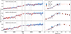 |
Fig. 1. Fit of the spectrum (left) and photometry (right) of an example galaxy for each cluster. The observed spectrum and photometry (in blue) and the corresponding best fit (in red) are shown. The shaded regions mark potential emission or telluric lines that are masked in the fit. |
Figure 2 illustrates the redshift dependence of the main physical parameters – age, mass, metallicity, and dust extinction – colour-coded by stellar velocity dispersion (σ★). The CC sample is characterised by high stellar masses, with a mean of log(M★/M⊙) = 11.2 ± 0.3, and, as expected, the stellar mass correlates positively with the velocity dispersion, such that the most massive galaxies also exhibit the highest σ★. The mass distribution is not uniform in redshift: higher-mass galaxies dominate the low-redshift end (z ≤ 0.55), whereas lower-mass systems become more prevalent at higher redshifts. This must be taken into account in the cosmological analysis of the age-redshift relation to ensure homogeneity across the subsamples used to trace population ageing.
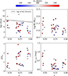 |
Fig. 2. Trends in redshift for the main physical parameters, colour-coded by the measured velocity dispersion. In the top-left panel, the solid line shows the age of the Universe computed in a flat ΛCDM with Ωm = 0.3. |
A qualitative inspection of the age-redshift trend already highlights two key results: evidence of mass downsizing (Thomas et al. 2010; Citro et al. 2017), with high-σ★ galaxies appearing systematically older than their low-σ★ counterparts, and a clear overall ageing trend of the CC sample, with stellar ages decreasing steadily towards higher redshifts in both the high- and low-σ★ populations. Even though no cosmological prior was adopted in the recovery of the galaxies’ ages, 95% of the sample is compatible with the age of the Universe in a flat ΛCDM (Ωm = 0.3) within the errors (∼0.4 Gyr on average). All objects are also characterised by short bursts of star formation, demonstrated by low values of the τ parameter, on average τ = 0.6 ± 0.2 Gyr. We find typically super-solar metallicities, with a mean value of Z/Z⊙ = 1.3 ± 0.7, but the sample spans the whole range 0–3 Z⊙. Dust reddening is predominantly low, with an average extinction in the V band of AV = 0.3 ± 0.3 mag.
4. Application to cosmology
Once the age–redshift relation for the sample of chronometers is derived, the CC method allows one to directly measure the Hubble parameter H(z) by evaluating the slope of this trend. In particular, the expansion rate can be expressed as
 (2)
(2)
where dz is the redshift difference between two adjacent bins and dt is the corresponding differential age. In practice, this requires a careful estimate of the CCs’ differential ages and a quantification of the associated statistical and systematic uncertainties.
In this work, we fixed the redshift of each galaxy to that of its parent cluster, namely z = 0.489, 0.542, and 0.588 (bins 0, 1, and 2, respectively). To evaluate the ageing of galaxies with comparable stellar masses, we divided the sample into two mass bins. As a threshold, we adopted log(M★/M⊙) = 11.05, which minimises the difference between the mean stellar masses of analogue subsamples. As already noted in the previous section, the mass distribution is not homogeneous: bins 0, 1, and 2 respectively contain 5, 17, and 1 CCs of the high-mass (HM) subsample (log(M★/M⊙) > 11.05) and 1, 6, and 7 galaxies of the low-mass (LM) subsample (log(M★/M⊙) ≤ 11.05). The last HM bin (HM2) and the first LM bin (LM0) had to be discarded because they both contained only one galaxy each. For this reason, we could evaluate the ageing of only two pairs of subsamples, HM0–HM1 and LM1–LM2, represented in the left panels of Fig. 3, to be combined into a single H(z) measurement.
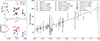 |
Fig. 3. Collection of all H(z) measurements obtained to date (Simon et al. 2005; Stern et al. 2010a; Moresco et al. 2012; Zhang et al. 2014; Moresco 2015; Moresco et al. 2016; Ratsimbazafy et al. 2017; Borghi et al. 2022b; Jiao et al. 2023; Tomasetti et al. 2023; Jiao et al. 2023; Loubser et al. 2025; Loubser 2025), including the result of this work. For comparison, the dashed line represents the flat ΛCDM trend from Planck18. The red shaded box shows the forecast on the precision achievable with a sample of 100 CCs (see Sect. 4.2 for details). |
To this end, we decided to adopt a bootstrap approach, which is described in detail in Appendix B. We generated N = 1000 perturbed realisations of the galaxy ages by sampling from Gaussian distributions centred on the best-fit ages and with a sigma equal to the age errors. For each realisation, we performed K = 1000 bootstrap re-samplings, computed the median ages in each mass-redshift bin, and derived age differences (dt) between adjacent bins. Converting those into H(z) via Eq. (2) and averaging the HM and LM results, we obtained N bootstrap realisations of H(z). The final value of H(z) and its statistical uncertainty are represented by the median and 16th and 84th percentiles of this distribution:

4.1. Systematic effects
With only 35 CCs, the statistical uncertainties are inevitably large and strongly dominate over systematics. Nevertheless, we wanted to include an estimate of systematic effects, following the results in Tomasetti et al. (2023), where the CC method was applied with the same FSF approach and a comparable sample size (39 CCs). In particular, the impact of the SFH was considered and found to affect H(z) at the ∼20% level. We stress, however, that this systematic contribution is likely overestimated as the effect of SFH fluctuations would be significantly reduced in larger samples. Considering this 20% as a conservative estimate of the systematics at play, and adding it in quadrature to the statistical component, we find
4.2. Future perspectives
As current and future facilities (e.g. Euclid and WST; Laureijs et al. 2011; Bacon et al. 2024) will deliver spectroscopic and photometric data for vast galaxy samples, it is timely to explore the potential gains from larger statistics. To this end, we estimated the precision achievable on H(z) with samples of different sizes, or different distributions, drawing synthetic age samples based on a flat ΛCDM cosmology, and applied the bootstrap procedure described at the beginning of this section to retrieve the H(z) measurement. In order to compare the results to this work, we considered the same division into two HM and two LM bins.
We performed various types of simulations, varying the distribution in redshift, the redshift coverage, and the statistics of the CC sample, to forecast the kind of statistical uncertainty achievable in future works. These simulations followed the bootstrap procedure described in Appendix B, with one modification: at step A of the algorithm, we generated random samples drawn from a Gaussian distribution centred on the age predicted by a flat ΛCDM cosmology for an object formed at redshift zf = 3 (for the HM sample) and zf = 1.5 (for the LM sample), with a dispersion of 0.5 Gyr.
In this work, we analysed a sample of 35 CCs unevenly distributed in four bins (with 5, 17, 6, and 7 galaxies, respectively), covering a redshift interval dz = 0.1. In these simulations, we tested three variations to this baseline: (A) homogenising the sample in redshift so that each bin has the same number (10) of CCs, (B) enlarging the redshift interval from dz = 0.1 to dz = 0.2, and (C) increasing the sample size to 100 CCs. In Fig. 4, we show the results of some of the tests performed, including different combinations of these three modifications.
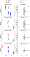 |
Fig. 4. Results of the simulations. Left column: For each setting, an example of an age–redshift relation for the HM (red) and LM (blue) samples, randomly extracted from a Gaussian distribution centred on the seed (black). Right column: Resulting H(z) distribution and the derived measurement (yellow star, also reported in the title), in comparison with the assumed cosmology (Planck Collaboration VI 2020). |
Interestingly, extending the redshift interval alone yielded the largest gain, with an error on H(z), compared to the one found in this work, reduced by ∼30%. Increasing the sample size also had a significant, though smaller, effect, reducing the error by ∼20%. Homogenising the distribution across bins had little impact on its own, but in combination with a wider redshift interval, it reduced the error by nearly 50%. As expected, combining all three improvements provided the strongest result, lowering the uncertainty on H(z) by approximately a factor of 4.
5. Conclusions
In this work we applied the CC method to measure the expansion history of the Universe, analysing VLT/MUSE data for the most massive, passively evolving galaxies in three galaxy clusters: SDSS 2222 (z = 0.49), MACS 1149 (z = 0.54), and SDSS 1029 (z = 0.59). Since MACS 1149 also hosts the multiply imaged SN Refsdal, previously used to infer H0 via TDC, our measurement of H(z) from the ageing of its member galaxies enabled a direct combination of complementary probes, thereby strengthening constraints on cosmological parameters.
We first selected the CC sample by combining a cut in stellar velocity dispersion, on their S/N, and on the H/K ratio to isolate the most massive and passive cluster members, ending up with a sample of 38 CCs. We then performed FSF with the Bagpipes code, which had been specifically modified to remove the cosmological prior on ages so that they could vary up to 15 Gyr. Despite this, 95% of the sample is compatible with the age of the Universe in a flat ΛCDM model and shows an ageing trend with redshift. Concerning the other physical parameters, the CC sample shows the characteristics of a passive population, with a high stellar mass (log(M★/M⊙) = 11.2 ± 0.3), a low dust extinction (AV = 0.3 ± 0.3 mag), and a short timescale of formation (τ = 0.6 ± 0.2 Gyr). The metallicity is on average super-solar, with a mean of Z/Z⊙ = 1.3 ± 0.7.
From the age–redshift relation, separating the HM and the LM galaxies (with log(M★/M⊙) = 11.05 as a threshold to ensure maximum homogeneity among subsamples), we measured H(z) by applying the CC method through a bootstrap approach, obtaining H(z = 0.542) =  (stat) ± 13 (syst). The error budget is currently dominated by the statistical component, but simulations show that with ∼100 CCs and an extended redshift interval of dz = 0.2, the statistical uncertainty could be reduced by up to 75%. Such an increase in precision would provide sufficiently tight constraints on H(z) that, when combined with TDC measurements, could significantly enhance their joint constraining power on cosmological parameters by breaking existing degeneracies (e.g. the H0–Ωm degeneracy; see Bergamini et al. 2024).
Future and upcoming surveys (e.g. Euclid, WST, MOONS, and LSST) will provide large samples of galaxies and galaxy clusters, offering unprecedented opportunities to apply the TDC method to strong lensing galaxy clusters, and the CC method to those cluster members with the required spectroscopic quality (or the necessary follow-up observations). Euclid (Laureijs et al. 2011), in particular, is expected to increase the census of strong gravitational lenses by orders of magnitude (Euclid Collaboration: Bergamini et al. 2026), opening the door to a systematic exploitation of this synergy.
Acknowledgments
We thank the anonymous referee for their constructive feedback, which helped us improve our manuscript. We also warmly thank Ana Acebron and Eros Vanzella for their useful and constructive feedback to this work. ET acknowledges the support from COST Action CA21136 “Addressing observational tensions in cosmology with systematics and fundamental physics (CosmoVerse)”, supported by COST (European Cooperation in Science and Technology). MMo acknowledges the financial contribution from the grant PRIN-MUR 2022 2022NY2ZRS 001 “Optimizing the extraction of cosmological information from Large Scale Structure analysis in view of the next large spectroscopic surveys” supported by Next Generation EU. MMo and AC acknowledge support from the grant ASI n. 2024-10-HH.0 “Attività scientifiche per la missione Euclid fase E”. The authors acknowledge support from the Italian Ministry of University and Research through grant PRIN-MIUR 2020SKSTHZ. MMe and PB were supported by INAF Grants “The Big-Data era of cluster lensing” and “Probing Dark Matter and Galaxy Formation in Galaxy Clusters through Strong Gravitational Lensing”, and ASI Grant n. 2024-10-HH.0 “Attività scientifiche per la missione Euclid fase E”. The research activities described in this paper have been co-funded by the European Union NextGeneration EU within PRIN 2022 project no. 20229YBSAN “Globular clusters in cosmological simulations and in lensed fields: from their birth to the present epoch”. SS has received funding from the European Union Horizon 2022 research and innovation programme under the Marie Skłodowska-Curie grant agreement No 101105167 – FASTIDIoUS.
References
- Acebron, A., Grillo, C., Bergamini, P., et al. 2022a, A&A, 668, A142 [NASA ADS] [CrossRef] [EDP Sciences] [Google Scholar]
- Acebron, A., Grillo, C., Bergamini, P., et al. 2022b, ApJ, 926, 86 [NASA ADS] [CrossRef] [Google Scholar]
- Bacon, R., Maineiri, V., Randich, S., et al. 2024, arXiv e-prints [arXiv:2405.12518] [Google Scholar]
- Bennett, C. L., Halpern, M., Hinshaw, G., et al. 2003, ApJS, 148, 1 [Google Scholar]
- Bergamini, P., Schuldt, S., Acebron, A., et al. 2024, A&A, 682, L2 [NASA ADS] [CrossRef] [EDP Sciences] [Google Scholar]
- Bertin, E., & Arnouts, S. 1996, A&AS, 117, 393 [NASA ADS] [CrossRef] [EDP Sciences] [Google Scholar]
- Borghi, N., Moresco, M., Cimatti, A., et al. 2022a, ApJ, 927, 164 [NASA ADS] [CrossRef] [Google Scholar]
- Borghi, N., Moresco, M., & Cimatti, A. 2022b, ApJ, 928, L4 [NASA ADS] [CrossRef] [Google Scholar]
- Bruzual, G., & Charlot, S. 2003, MNRAS, 344, 1000 [NASA ADS] [CrossRef] [Google Scholar]
- Buchner, J. 2016, Stat. Comput., 26, 383 [Google Scholar]
- Calzetti, D., Armus, L., Bohlin, R. C., et al. 2000, ApJ, 533, 682 [NASA ADS] [CrossRef] [Google Scholar]
- Cappellari, M. 2023, MNRAS, 526, 3273 [NASA ADS] [CrossRef] [Google Scholar]
- Cardelli, J. A., Clayton, G. C., & Mathis, J. S. 1989, ApJ, 345, 245 [Google Scholar]
- Carnall, A. C., McLure, R. J., Dunlop, J. S., & Davé, R. 2018, MNRAS, 480, 4379 [Google Scholar]
- Carnall, A. C., McLure, R. J., Dunlop, J. S., et al. 2019, MNRAS, 490, 417 [Google Scholar]
- Citro, A., Pozzetti, L., Quai, S., et al. 2017, MNRAS, 469, 3108 [Google Scholar]
- Di Valentino, E., Said, J. L., Riess, A., et al. 2025, Phys. Dark Universe, 49, 101965 [Google Scholar]
- Eisenstein, D. J., Zehavi, I., Hogg, D. W., et al. 2005, ApJ, 633, 560 [Google Scholar]
- Euclid Collaboration (Bergamini, P., et al.) 2026, A&A, in press, https://doi.org/10.1051/0004-6361/202554577 [Google Scholar]
- Gonneau, A., Lyubenova, M., Lançon, A., et al. 2020, A&A, 634, A133 [NASA ADS] [CrossRef] [EDP Sciences] [Google Scholar]
- Granata, G., Caminha, G. B., Ertl, S., et al. 2025, A&A, 697, A94 [NASA ADS] [CrossRef] [EDP Sciences] [Google Scholar]
- Grillo, C., Karman, W., Suyu, S. H., et al. 2016, ApJ, 822, 78 [Google Scholar]
- Grillo, C., Rosati, P., Suyu, S. H., et al. 2018, ApJ, 860, 94 [Google Scholar]
- Grillo, C., Rosati, P., Suyu, S. H., et al. 2020, ApJ, 898, 87 [Google Scholar]
- Grillo, C., Pagano, L., Rosati, P., & Suyu, S. H. 2024, A&A, 684, L23 [NASA ADS] [CrossRef] [EDP Sciences] [Google Scholar]
- Ivezić, Z., Kahn, S. M., Tyson, J. A., et al. 2019, ApJ, 873, 111 [NASA ADS] [CrossRef] [Google Scholar]
- Jiao, K., Borghi, N., Moresco, M., & Zhang, T.-J. 2023, ApJS, 265, 48 [NASA ADS] [CrossRef] [Google Scholar]
- Jimenez, R., & Loeb, A. 2002, ApJ, 573, 37 [NASA ADS] [CrossRef] [Google Scholar]
- Kamionkowski, M., & Riess, A. G. 2023, Ann. Rev. Nucl. Part. Sci., 73, 153 [NASA ADS] [CrossRef] [Google Scholar]
- Kelly, P. L., Rodney, S. A., Treu, T., et al. 2015, Science, 347, 1123 [Google Scholar]
- Kelly, P. L., Rodney, S., Treu, T., et al. 2023, ApJ, 948, 93 [NASA ADS] [CrossRef] [Google Scholar]
- Kroupa, P. 2001, MNRAS, 322, 231 [NASA ADS] [CrossRef] [Google Scholar]
- La Barbera, F., de Carvalho, R. R., Gal, R. R., et al. 2005, ApJ, 626, L19 [Google Scholar]
- Laureijs, R., Amiaux, J., Arduini, S., et al. 2011, arXiv e-prints [arXiv:1110.3193] [Google Scholar]
- Lotz, J. M., Koekemoer, A., Coe, D., et al. 2017, ApJ, 837, 97 [Google Scholar]
- Loubser, S. I. 2025, MNRAS, 544, 3064 [Google Scholar]
- Loubser, S. I., Alabi, A. B., Hilton, M., et al. 2025, MNRAS, 540, 3135 [Google Scholar]
- Mignoli, M., Zamorani, G., Scodeggio, M., et al. 2009, A&A, 493, 39 [NASA ADS] [CrossRef] [EDP Sciences] [Google Scholar]
- Moresco, M. 2015, MNRAS, 450, L16 [NASA ADS] [CrossRef] [Google Scholar]
- Moresco, M., Cimatti, A., Jimenez, R., et al. 2012, JCAP, 2012, 006 [CrossRef] [Google Scholar]
- Moresco, M., Pozzetti, L., Cimatti, A., et al. 2016, JCAP, 2016, 014 [CrossRef] [Google Scholar]
- Moresco, M., Jimenez, R., Verde, L., et al. 2018, ApJ, 868, 84 [NASA ADS] [CrossRef] [Google Scholar]
- Moresco, M., Amati, L., Amendola, L., et al. 2022, Liv. Rev. Relat., 25, 6 [NASA ADS] [Google Scholar]
- Oguri, M., Schrabback, T., Jullo, E., et al. 2013, MNRAS, 429, 482 [NASA ADS] [CrossRef] [Google Scholar]
- Peletier, R. F., Davies, R. L., Illingworth, G. D., Davis, L. E., & Cawson, M. 1990, AJ, 100, 1091 [Google Scholar]
- Peng, C. Y., Ho, L. C., Impey, C. D., & Rix, H.-W. 2002, AJ, 124, 266 [Google Scholar]
- Peng, C. Y., Ho, L. C., Impey, C. D., & Rix, H.-W. 2010, AJ, 139, 2097 [Google Scholar]
- Perlmutter, S., Aldering, G., Goldhaber, G., et al. 1999, ApJ, 517, 565 [Google Scholar]
- Petrecca, V., Botticella, M. T., Cappellaro, E., et al. 2024, A&A, 686, A11 [NASA ADS] [CrossRef] [EDP Sciences] [Google Scholar]
- Planck Collaboration VI. 2020, A&A, 641, A6 [NASA ADS] [CrossRef] [EDP Sciences] [Google Scholar]
- Pozzetti, L., Bolzonella, M., Zucca, E., et al. 2010, A&A, 523, A13 [NASA ADS] [CrossRef] [EDP Sciences] [Google Scholar]
- Ratsimbazafy, A. L., Loubser, S. I., Crawford, S. M., et al. 2017, MNRAS, 467, 3239 [NASA ADS] [CrossRef] [Google Scholar]
- Riess, A. G., Filippenko, A. V., Challis, P., et al. 1998, AJ, 116, 1009 [Google Scholar]
- Salim, S., Boquien, M., & Lee, J. C. 2018, ApJ, 859, 11 [Google Scholar]
- Schuldt, S., Grillo, C., Caminha, G. B., et al. 2024, A&A, 689, A42 [NASA ADS] [CrossRef] [EDP Sciences] [Google Scholar]
- Sharon, K., Bayliss, M. B., Dahle, H., et al. 2017, ApJ, 835, 5 [NASA ADS] [CrossRef] [Google Scholar]
- Simon, J., Verde, L., & Jimenez, R. 2005, Phys. Rev. D, 71, 123001 [NASA ADS] [CrossRef] [Google Scholar]
- Stern, D., Jimenez, R., Verde, L., Kamionkowski, M., & Stanford, S. A. 2010a, JCAP, 2010, 008 [Google Scholar]
- Stern, D., Jimenez, R., Verde, L., Stanford, S. A., & Kamionkowski, M. 2010b, ApJS, 188, 280 [NASA ADS] [CrossRef] [Google Scholar]
- Suyu, S. H., Acebron, A., Grillo, C., et al. 2026, A&A, in press, https://doi.org/10.1051/0004-6361/202557235 [Google Scholar]
- TDCOSMO Collaboration (Birrer, S., et al.) 2025, A&A, 704, A63 [Google Scholar]
- Thomas, D., Maraston, C., Schawinski, K., Sarzi, M., & Silk, J. 2010, MNRAS, 404, 1775 [NASA ADS] [Google Scholar]
- Tomasetti, E., Moresco, M., Borghi, N., et al. 2023, A&A, 679, A96 [NASA ADS] [CrossRef] [EDP Sciences] [Google Scholar]
- Tomasetti, E., Moresco, M., Lardo, C., Cimatti, A., & Jimenez, R. 2025, A&A, 696, A98 [NASA ADS] [CrossRef] [EDP Sciences] [Google Scholar]
- Tortorelli, L., & Mercurio, A. 2023, Front. Astron. Space Sci., 10, 51 [NASA ADS] [CrossRef] [Google Scholar]
- Tortorelli, L., Mercurio, A., Granata, G., et al. 2023, A&A, 671, L9 [NASA ADS] [CrossRef] [EDP Sciences] [Google Scholar]
- Weilbacher, P. M., Palsa, R., Streicher, O., et al. 2020, A&A, 641, A28 [NASA ADS] [CrossRef] [EDP Sciences] [Google Scholar]
- Williams, R. J., Quadri, R. F., Franx, M., van Dokkum, P., & Labbé, I. 2009, ApJ, 691, 1879 [NASA ADS] [CrossRef] [Google Scholar]
- Zhang, C., Zhang, H., Yuan, S., et al. 2014, Res. Astron. Astrophys., 14, 1221 [CrossRef] [Google Scholar]
It will be important in future works to assess the impact of adopting models with different levels of α-enhancement, which could lead to younger inferred ages. However, differential ages should remain largely unaffected, provided that the sample is homogeneous.
Morphofit: a Python package, based on Galfit (Peng et al. 2002, 2010) and Sextractor (Bertin & Arnouts 1996), for the morphological analysis of galaxies. See https://github.com/torluca/morphofit
Appendix A: Observations
MUSE coverage of the central regions of MACS 1149 was granted by the DDT programme 294.A-5032 (P.I. C. Grillo), for a total integration time of 6h and seeing of less than 1.1″ in almost all exposures (Grillo et al. 2016), complemented by 5.5 h of observations of the north-west region of the cluster within the programme 105.20P5 (P.I. A. Mercurio), presented in Schuldt et al. (2024). SDSS 1029 was observed with MUSE under the programme 0102.A-0642(A) (P.I. C. Grillo), presented in Acebron et al. (2022b), with a total exposure time of 4.8 h and a full width at half maximum of 0.71″. SDSS 2222 was targeted with the integral field spectrograph MUSE at the VLT, under programme 0103.A-0554(A) (P.I. C. Grillo), presented in Acebron et al. (2022a) for a cumulative exposure time of 4.4 h. We used the MUSE data-reduction pipeline version v2.8.5 (Weilbacher et al. 2020) for all observations to build the final data cube.
We used archival HST multi-colour imaging from the ACS and WFC3. SDSS 2222 (GO-13337; P.I. Sharon) was imaged over two orbits in each of the ACS filters F475W, F606W, and F814W, while the WFC3 imaging in F110W and F160W was allocated one single orbit in total. SDSS 1029 (GO-12195; P.I. Oguri) was imaged over two orbits in F475W, three orbits in F814W, and two orbits in the WFC3 filter F160W. A detailed description of the observations and data reduction process is available in Sharon et al. (2017), Oguri et al. (2013). For MACS 1149, the photometric data belong to the Frontier Fields program (P.I. J. Lotz, Lotz et al. 2017), while the data reduction is widely described in Tortorelli et al. (2023). For each cluster, we extracted a photometric catalogue using Morphofit2 (Tortorelli & Mercurio 2023). We also investigated how the choice of aperture size affects the extraction of 1D spectra from MUSE data cubes. For a subset of galaxies, we extracted their spectra from the data cube using circular apertures of 0.5″, 0.8″, 1.0″, and 1.6″ of radius. As shown in Fig. A.1, we found that the shape of the 1D spectrum varies with the aperture size. Specifically, a smaller extraction aperture tends to produce a redder spectrum compared to one extracted using a larger aperture (namely, the spectrum shows an increase in flux at longer wavelengths). This is not unexpected, since often early-type galaxies show colour gradients due to, for example, a lower metallicity of the stars inhabiting the galaxy outskirts compared to the ones that are in the central region (e.g. Peletier et al. 1990; La Barbera et al. 2005). This effect can cause a non-negligible mismatch between the galaxy spectrum and the photometry when different apertures are used, negatively impacting the quality of the FSF. For this reason, we also allowed Bagpipes to perform a calibration of the spectrum by multiplying it with a second-order Chebyshev polynomial and, with the coefficients optimised during the fitting process, to achieve a better match of the spectrum with the photometry.
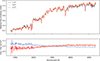 |
Fig. A.1. Example showing the effect of the aperture sizes on the extraction of a 1D spectrum from a MUSE data cube. Top: Spectrum of the same member of the cluster SDSS 2222, extracted using circular apertures of radius 1.4″ (blue), 0.6″ (orange), and 0.3″ (red). Bottom: Ratio between each spectrum and the one extracted with the 0.3″ aperture. A bigger extraction aperture produces a bluer spectrum (namely, the spectrum shows a larger flux at lower wavelengths). |
Appendix B: Bootstrap algorithm
In Fig. B.1, the workflow of the bootstrap algorithm used to obtain the final H(z) measurement is illustrated. Each cycle is repeated a thousand times (N = K = 1000).
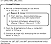 |
Fig. B.1. Visual diagram of the bootstrap algorithm. The CC sample was divided into three redshift bins (0, 1, and 2) and into two mass bins, HM and LM, but only bins HM0, HM1, LM1, and LM2 had enough statistics to be used. |
We generated N = 1000 perturbed realisations of the galaxy ages by sampling each object from a Gaussian distribution centred on its best-fit age and with a standard deviation equal to its uncertainty. From each of these perturbed arrays, we extracted with repetition K = 1000 samples with the same numerosity, computed the K median ages in each mass–redshift bin, and estimated the age differences dt between adjacent bins of the same mass. This process generated N bootstrap distributions of dt, each with K realisations, for both the high- and the low-redshift intervals. For each case, we extracted the median of dt, derived two independent measurements of H(z) applying Eq. 2, and combined them into a single measurement by averaging the values. The final value of H(z) and its statistical uncertainty are represented by the median and 16th and 84th percentiles of these N realisations.
All Tables
All Figures
|
Fig. 1. Fit of the spectrum (left) and photometry (right) of an example galaxy for each cluster. The observed spectrum and photometry (in blue) and the corresponding best fit (in red) are shown. The shaded regions mark potential emission or telluric lines that are masked in the fit. |
| In the text | |
|
Fig. 2. Trends in redshift for the main physical parameters, colour-coded by the measured velocity dispersion. In the top-left panel, the solid line shows the age of the Universe computed in a flat ΛCDM with Ωm = 0.3. |
| In the text | |
|
Fig. 3. Collection of all H(z) measurements obtained to date (Simon et al. 2005; Stern et al. 2010a; Moresco et al. 2012; Zhang et al. 2014; Moresco 2015; Moresco et al. 2016; Ratsimbazafy et al. 2017; Borghi et al. 2022b; Jiao et al. 2023; Tomasetti et al. 2023; Jiao et al. 2023; Loubser et al. 2025; Loubser 2025), including the result of this work. For comparison, the dashed line represents the flat ΛCDM trend from Planck18. The red shaded box shows the forecast on the precision achievable with a sample of 100 CCs (see Sect. 4.2 for details). |
| In the text | |
|
Fig. 4. Results of the simulations. Left column: For each setting, an example of an age–redshift relation for the HM (red) and LM (blue) samples, randomly extracted from a Gaussian distribution centred on the seed (black). Right column: Resulting H(z) distribution and the derived measurement (yellow star, also reported in the title), in comparison with the assumed cosmology (Planck Collaboration VI 2020). |
| In the text | |
|
Fig. A.1. Example showing the effect of the aperture sizes on the extraction of a 1D spectrum from a MUSE data cube. Top: Spectrum of the same member of the cluster SDSS 2222, extracted using circular apertures of radius 1.4″ (blue), 0.6″ (orange), and 0.3″ (red). Bottom: Ratio between each spectrum and the one extracted with the 0.3″ aperture. A bigger extraction aperture produces a bluer spectrum (namely, the spectrum shows a larger flux at lower wavelengths). |
| In the text | |
|
Fig. B.1. Visual diagram of the bootstrap algorithm. The CC sample was divided into three redshift bins (0, 1, and 2) and into two mass bins, HM and LM, but only bins HM0, HM1, LM1, and LM2 had enough statistics to be used. |
| In the text | |
Current usage metrics show cumulative count of Article Views (full-text article views including HTML views, PDF and ePub downloads, according to the available data) and Abstracts Views on Vision4Press platform.
Data correspond to usage on the plateform after 2015. The current usage metrics is available 48-96 hours after online publication and is updated daily on week days.
Initial download of the metrics may take a while.