| Issue |
A&A
Volume 708, April 2026
|
|
|---|---|---|
| Article Number | A85 | |
| Number of page(s) | 9 | |
| Section | Astronomical instrumentation | |
| DOI | https://doi.org/10.1051/0004-6361/202558344 | |
| Published online | 30 March 2026 | |
Jitter sensing and reconstruction from temporal series of solar images: Applications to TuMag
1
Instituto de Astrofísica de Andalucía, CSIC, Glorieta de la Astronomía s/n, 18008 Granada, Spain
2
Spanish Space Solar Physics Consortium (S3PC), https://s3pc.es, Spain
3
Max-Planck-Institut für Sonnensystemforschung, Justus-von-Liebig-Weg 3, 37077 Göttingen, Germany
4
Aalto University, Department of Computer Science, Konemiehentie 2, 02150 Espoo, Finland
5
National Astronomical Observatory of Japan, 2-21-1 Osawa, Mitaka, Tokyo 181-8588, Japan
6
Department of Earth and Planetary Science, The University of Tokyo, 7-3-1, Hongo, Bunkyo-ku, Tokyo 113-0033, Japan
7
Department of Astronomical Science, The Graduate University for Advanced Studies (SOKENDAI), 2-21-1 Osawa, Mitaka, Tokyo 1818588, Japan
8
Johns Hopkins Applied Physics Laboratory, 11100 Johns Hopkins Road, Laurel, MD, USA
9
Institut für Sonnenphysik (KIS), Georges-Köhler-Allee 401a, 79110 Freiburg, Germany
10
Instituto Nacional de Técnica Aeroespacial (INTA), Ctra. de Ajalvir, km. 4, 28850 Torrejón de Ardoz, Spain
11
National Solar Observatory, 3665 Discovery Drive, Boulder, CO 80303, USA
12
Universitat de Valencia Catedrático José Beltrán 2, 46980 Paterna-Valencia, Spain
13
Instituto Universitario “Ignacio da Riva”. Universidad Politécnica de Madrid. (IDR-UPM), Plaza Cardenal Cisneros 3, 28040 Madrid, Spain
14
Instituto de Astrofísica de Canarias, Vía Láctea s/n, 38205 La Laguna, Spain
15
Laboratory for Atmospheric and Space Physics (LASP), University of Colorado Boulder, CO, USA
16
Geophysical and Astronomical Observatory, Faculty of Science and Technology, University of Coimbra, Portugal
17
Centre for Integrated Data Science, Institute for Space-Earth Environmental Research, Nagoya University, Furocho, Chikusa-ku, Nagoya, Aichi 464-8601, Japan
18
National Institute for Fusion Science, 322-6 Oroshi-cho, Toki City 509-5292, Japan
19
Grupo de Estudios en Heliofísica de Mendoza, CONICET, Universidad de Mendoza, Boulogne sur Mer 683, 5500 Mendoza, Argentina
20
Institut für Physik, Universität Graz, Universitätsplatz 5, 8010 Graz, Austria
21
Advanced Research Center for Space Science and Technology, Institute of Science and Engineering, Kanazawa University, Kakuma-machi, Kanazawa, Ishikawa 920-1192, Japan
★ Corresponding author: This email address is being protected from spambots. You need JavaScript enabled to view it.
Received:
1
December
2025
Accepted:
4
February
2026
Abstract
Context. Images recorded with the Tunable Magnetograph (TuMag) instrument on board the SUNRISE III balloon observatory are affected by temporal contrast fluctuations. These variations are related to high-frequency vibrations (jitter) of the platform that cannot be entirely compensated by the image stabilization unit of the telescope. Jitter smooths out mid- to high-frequency details and degrades the contrast of images that are integrated over hundreds of milliseconds to achieve the signal-to-noise levels required by the instrument. The temporal variations of jitter hamper the reconstruction of the data and limit the accuracy of the instrument.
Aims. We present a technique that allows us to infer and compensate temporal changes of the amplitude and direction of jitter from two images of the same scene, provided they are recorded close enough in time to prevent the scene from evolving significantly.
Methods. We assess the performance of our method through a dynamical magnetohydrodynamical simulation of the solar scene that is degraded with diffraction effects, noise, and jitter. We evaluate the performance of the algorithm as a function of the jitter amplitude and as a function of the time gap between the two images. We finally apply it to a time series recorded by TuMag to sense and restore the temporal evolution of jitter on the images.
Results. Our numerical experiments show that the algorithm is able to sense jitter with an accuracy better than 0.″005 (≲0.1 px) for images recorded less than 10 s apart and assuming a worst-case scenario with a low signal-to-noise ratio of 100 and induced rms jitter amplitudes as large as 0.″15 in the X and Y directions. When increasing the time interval to 30 s, the errors found are still below 0.″01. For the chosen TuMag series we find that the jitter rms amplitudes vary strongly within the range 0.″05–0.″15 (∼1–4 px) and are anticorrelated to the contrast of the recorded images. Correction of jitter improves the contrast of wavefront-reconstructed images by 2.5% in some cases and reduces the rms variation of contrast along the series by half.
Key words: magnetohydrodynamics (MHD) / techniques: image processing / telescopes
© The Authors 2026
 Open Access article, published by EDP Sciences, under the terms of the Creative Commons Attribution License (https://creativecommons.org/licenses/by/4.0), which permits unrestricted use, distribution, and reproduction in any medium, provided the original work is properly cited.
This article is published in open access under the Subscribe to Open model. This email address is being protected from spambots. You need JavaScript enabled to view it. to support open access publication.
1 Introduction
Vibrations in astronomical telescopes introduce differential shifts between consecutive images recorded by the instruments they carry, smearing out high-frequency details and reducing the resolution and contrast of the data. These vibrations are often referred to as “jitter”.
Jitter is particularly important in imaging spectropolarimeters. These instruments combine images with different intensity modulations to produce maps of the incident Stokes vector at selected wavelengths. Any vibrations of the focal plane that occur during polarimetric measurements introduce spurious signals in the inferred state of polarization. Therefore, accurate pointing and image stabilization systems are often needed to achieve the required polarimetric sensitivities.
If images are recorded quickly enough (with an integration time of a few milliseconds), residual jitter mostly manifests as a shift in the image, which can be corrected to a large extent using post-alignment techniques (e.g., Guizar-Sicairos et al. 2008). However, residual vibrations with kilohertz frequencies will still influence the optical quality of the images and must be compensated for using real-time image reconstruction algorithms (e.g., the Multi-Object Multi-Frame Blind Deconvolution, MOMFBD, technique developed by van Noort et al. 2005). Exposure times of a few milliseconds combined with real-time wavefront sensing methods are difficult to achieve for spaceborne instruments due to the stringent data rate and volume requirements imposed by the platform. Therefore, an alternative approach must be adopted to correct for any residual jitter. This technique is presented here and is tested on data obtained by the Tunable Magnetograph (TuMag) instrument (Del Toro Iniesta et al. 2025) on board the SUNRISE III mission (Korpi-Lagg et al. 2025).
TuMag is a tunable imaging spectropolarimeter capable of mapping the full Stokes vector of the solar photosphere and the low cromosphere over a field of view (FoV) of 63″ × 63″ and along several spectral lines sensitive to the magnetic field. The instrument allows quasi-simultaneous observations of the Stokes vector for different combinations of two of the following lines: Fe I 525.02 nm, Fe I 525.06 nm, and Mg I b2 517.3 nm. The magnetic field and the line-of-sight velocities of the plasma can be inferred at different heights of the solar photosphere from these observations to study its dynamic coupling.
SUNRISE III is a stratospheric balloon observatory launched in the summer of 2024 from the Esrange Space Center of the Swedish Space Corporation (SSC) in northern Sweden. The mission flew for 6.5 days over the Arctic Circle, providing continuous observations of the solar atmosphere with three instruments that operate in different bands: SUSI (Feller et al. 2025; Iglesias et al. 2025) in the near ultraviolet, TuMAG in the visible, and SCIP (Katsukawa et al. 2025) in the near infrared.
SUNRISE III is equipped with a 1m-class telescope (Barthol et al. 2011) that already flew twice successfully in 2009 and 2013 (Solanki et al. 2010, 2017). It provides diffraction-limited spatial resolution in the ultraviolet (0.″03), visible (0. ″05), and infrared ranges (0.″09). To reach these spatial resolutions and a polarimetric sensitivity of 10−3, the telescope must provide an image stability better than 0.″005 rms at its focal plane. Different dedicated subsystems are implemented for this purpose. The gondola is equipped with a pointing system with an accuracy of 15″ (Bernasconi et al. 2025). The residual vibrations of the platform are then corrected by an image stabilization unit (ISU) that detects shifts on the focal plane of the telescope with milliarc-second accuracy through a correlating wavefront sensor (CWS) and counteracts it by means of a fast tip-tilt mirror (Berkefeld et al. 2025).
Fulfilling the tight requirements on image stability by the ISU along the full mission is extremely challenging, especially due to the hard environmental conditions to which the observatory has been exposed. Residual high-frequency vibrations not fully corrected by the ISU (jitter) rapidly shift the position of the focal plane. The impact of these vibrations on the image quality is negligible in the near infrared (SCIP) and can be overcome at shorter wavelengths by reducing the exposure time of the recorded images down to a few milliseconds (SUSI). Post alignment of the individual short-exposure images with subpixel accuracy eliminates any relative shifts between them.
The high data rate produced by TuMag and the restrictions on the data volume imposed by the mission prevent this instrument from following the same strategy. Instead, TuMag accumulates several short-exposure (42 ms) images in most observation modes to get an effective integration time of a few hundreds of milliseconds in order to reach a signal-to-noise ratio (S/N) of 1700 at the continuum of Stokes I and therefore a polarimetric sensitivity of 10−3 in Stokes Q, U, and V (Del Toro Iniesta & Martínez Pillet 2012). When integrated over such long times, the accumulated effect of the residual vibrations is a blurring of mid- to high-frequency details in the images, with a subsequent decrease of image contrast.
The amount of residual jitter not corrected by the ISU changes over the mission and is often above the image stability requirement. In some cases, the quiet-sun granulation contrast of nonreconstructed data recorded by TuMag varies from ∼8% to ∼10%, with occasional steep jumps between two consecutive images. These fluctuations are much smaller than those observed in ground instrumentation, and the mean contrast values are comparable – and even better in some cases – than those obtained in previous SUNRISE flights.
TuMag makes use of the Phase Diversity (PD) wavefront-sensing technique (Gonsalves & Chidlaw 1979; Paxman et al. 1992; Löfdahl & Scharmer 1994) to compensate for the aberrations introduced by the telescope, the image stabilization and light distribution unit (ISLiD), and the instrument itself. This method usually employs a pair of focused-defocused images and their corresponding optical transfer functions (OTFs) to construct a merit function. The images differ only by a difference of phase related to the amount of (known) defocus – the “phase diversity”. Their OTFs are parameterized as a function of a finite set of Zernike coefficients, which can be left as free parameters and optimized through nonlinear optimization methods.
In TuMag, the images of a PD pair are recorded sequentially thanks to a filter wheel that contains an empty hole to acquire the focused image and a plane-parallel glass to produce the desired defocus on the other one (Bailén et al. 2022a). The wavefront error (WFE) is determined periodically during selected calibration windows along the mission and is used to restore the closest images recorded by the instrument. Since aberrations and science data are not recorded simultaneously, temporal changes in the contrast caused by residual jitter cannot be sensed through PD and therefore compensated by restoring the wavefront error.
To include the effect of residual vibrations on the reconstructions, we have designed a tailored algorithm that senses the rms amplitude of jitter and its correlation along the X and Y directions at a given time from two sequential images. Our technique is inspired by the PD method and remains valid for any instrument that shows contrast fluctuations along time as a result of jitter. Unlike traditional PD, our algorithm uses two focused images whose OTFs differ only by a jitter term that can be fitted. This additional term is modeled as a Gaussian OTF that contains information on the statistical distribution of shifts accumulated over the integration time (e.g., Johnson 1993; Pittelkau & McKinley 2016; Fiete & Paul 2014).
Our work is structured as follows. In Sect. 2, we introduce our method. In Sect. 3, we study the performance of the algorithm against synthetic data. In Sect. 4, we infer the amplitude and direction of jitter with our method and we compensate it along a selected time series recorded by TuMag. Finally, we summarize our main conclusions in Section 5.
2 Method
The recorded image, f (x, y), of an extended object, o(x, y), in an isoplanatic – invariant against translations – optical system for spatially incoherent illumination can be modelled as (e.g., Born & Wolf 1999)
 (1)
(1)
where ∗ is the convolution operator, s(x, y) is the point spread function (PSF) of the system, and n(x, y) is an additive noise term. In the Fourier domain, this relation can be expressed simply as
 (2)
(2)
where capital letters refer to the Fourier transform of the lowercase variables of Eq. (1) and (u, v) are the frequency coordinates in the Fourier domain. The Fourier transform of the PSF, S (u, v), is known as the OTF of the system.
High-frequency vibrations of a telescope or its instruments are usually known as jitter and produce translations of the image on the focal plane that change over time. These shifts can be modeled by introducing a phase constant on the OTF as in the way
![Mathematical equation: ${S_{{\rm{shift}}}}(u,v,{\rm{\Delta }}x,{\rm{\Delta }}y) = {S_{{\rm{wave}}}}(u,v)\exp [ - {\rm{i}}(u{\rm{\Delta }}x + v{\rm{\Delta }}y)],$](/articles/aa/full_html/2026/04/aa58344-25/aa58344-25-eq3.png) (3)
(3)
where Swave(u, v) is the OTF of the system before the image is displaced, including diffraction effects and aberrations, and ∆x and ∆y are the shifts along the X and Y directions produced by the jitter in a particular instant.
When the exposure time of the image is much longer than the timescale associated with these vibrations, the net effect on the image is equivalent to temporally averaging Sshift over the integration time of the instrument. Assuming that shifts vary following a normal bi-variate distribution with an rms deviation σx and σy and a correlation factor ρxy along the X and Y directions, the “effective” OTF, Seff, is given simply by
 (4)
(4)
where Sjitt is the time average of the shift term in Equation (3). This jitter term can be approximated as an exponential function of the type (Fiete & Paul 2014)
![Mathematical equation: ${S_{{\rm{jitt}}}}(u,v) = \exp \left[ { - 2{\pi ^2}\left( {\sigma _x^2{u^2} + \sigma _y^2{v^2} + 2{\rho _{xy}}{\sigma _x}{\sigma _y}uv} \right)} \right].$](/articles/aa/full_html/2026/04/aa58344-25/aa58344-25-eq5.png) (5)
(5)
We now assume that two images of the same scene, f1 and f2, are recorded by the instrument at different times, each of them affected by a different rms jitter amplitude. The corresponding OTFs are given by Seff,i = SwaveSjitt,i, where Sjitt,i ≡ Sjitt(σx,i, σy,i, ρxy,i) and i = 1, 2. Following Paxman et al. (1992), the maximum likelihood estimate of the object – assuming that noise follows a Gaussian distribution – occurs when the merit function
 (6)
(6)
is minimized. The amplitude and direction of the jitter can therefore be determined if the values of σx,i, σy,i, and ρxy,i that minimize this equation are found. To deal with edge effects and artifacts arising from the numerical computation of the Fourier transforms, optimization can be carried out in much the same way as the Phase Diversity algorithm of Löfdahl & Scharmer (1994), except that in this case there is no phase difference among the two images and the parameters describing the two OTFs are fitted independently.
Note also that the OTF term Swave cancels out in Eq. (6) because we have assumed optical aberrations to be the same between the two images. This assumption generally holds for space-based and stratospheric balloon-borne instruments, even when images are not acquired simultaneously, because the wavefront error remains approximately static over time. Under these conditions, jitter and wavefront sensing can be treated as independent problems. Once jitter and wavefront aberrations are inferred, the images can be reconstructed using their effective OTF and an appropriate noise filter to minimize its amplification at certain frequencies.
3 Numerical experiments
We used a set of synthetic magnetohydrodynamical (MHD) simulations carried out with the MURaM code (Vögler et al. 2005) that evolve over 40 s in 1 s steps to validate our method. The simulations cover a 14″ × 14″ field of view with an angular resolution of 0.″055, equivalent to the plate scale of the IMaX instrument (Martínez Pillet et al. 2011) on board the SUNRISE I and II missions (Solanki et al. 2010, 2017).
To simulate jitter, we accumulate 1000 images affected by shifts that follow a standard (uncorrelated) bi-variate normal distribution with the same rms deviation along the X and Y directions (σx,true = σy,true). The images are degraded by the diffraction-limited PSF of a 1-m class telescope with a central obscuration of 32.4% working at 525 nm to simulate SUNRISE telescope (Barthol et al. 2011). We evaluate our method under two scenarios: that the images are free from noise and that they are affected by Gaussian noise distribution, producing a S/N of 100. We consider the latter a worst-case scenario for imaging spectropolarimeters such as TuMag.
We adapted the PD algorithm presented in Bailén et al. (2022b) to infer the amount of jitter following Section 2. In this way we ensure that edge effects inherent to the use of fast Fourier transforms (FFTs) and noise amplification are suitably dealt with. We chose a Nelder–Mead algorithm to minimize Eq. (6), as we found this method to be robust enough to sense jitter while not requiring knowledge of the analytical derivatives of the merit function. We used bounds σx > 0, σy > 0, and 0 < ρxy < 1 to guaranty that the solution has a physical meaning and to help the algorithm find the global minimum. The codes were developed in Python and are publicly available1.
Figure 1 shows the noiseless MHD simulation at the initial time before and after being degraded by the diffraction-limited PSF of the telescope, as well as after inducing jitter with rms amplitudes σx,true = σy,true = 0.″1 (≃1.8 px). The corresponding contrasts computed as the ratio between the rms of the images and their mean value over the whole FoV are displayed, also. Note that the contrast decreases from 24.2% to 17.5% simply due to the diffraction effects of the telescope. When including jitter, the middle and high-frequency (small-scale) details are further smoothed out, so the contrast is reduced even further to 15.5%.
We induced 1000 different realizations of jitter in the synthetic data at the initial time of the simulations and varied σx,true = σy,true from 0 to 0.″15 (∼2.7 px) to study the accuracy of our algorithm with the amount of jitter. We then minimized Eq. (6) using a reference image unaffected by jitter and the jit-tered image, for which Sjitt is fitted. Figure 2 shows the norm of the inferred jitter,  , against the simulated (“true”) one,
  . The noiseless and S/N = 100 cases are shown in the top and bottom panels, respectively. The density of points is represented with a gradient of colors: yellowish zones correspond to high-density areas, whereas blueish zones represent low-density areas.
When simulations are free from noise, there is an almost one-to-one correspondence between inferred and true jitter up to ∼0.″1 (≃1.8 px). The accuracy begins to worsen from there, with errors that can be as large as ∼0.″05 (∼0.9 px) in some cases. Note that the inferred jitter is usually underestimated from σtrue ≃ 0.″15 on. The opposite happens when images are affected by noise. In this case, the algorithm is more prone to errors when σtrue is very small (below ∼0.″01), but it proves to be very robust above ∼0.″01. Deviations from the true value are typically below 0.″003 in this scenario, except for a few isolated cases. This suggests that noise somehow helps the algorithm to constrain the solution towards the true one above a certain threshold.
The performance of the algorithm is also expected to be affected by the time gap between the images as the solar scene evolves on timescales of a few seconds. We computed the norm of the residual jitter, ∆σ, as a function of the time interval between images for a S/N = 100 and for different amounts of induced jitter (σx,true = σy,true = 0″, 0.″05, 0.″10, and 0.″15), where ∆σ is defined as
 (7)
(7)
We ran 100 realizations of noise and jitter per time unit (1 s) for each choice of σtrue to assess the accuracy and robustness of the algorithm. We then minimized Eq. (6) using the jittered image and a jitter-free reference scene corresponding to the initial simulation time. The values of the jitter rms amplitude were fitted only for the image affected by it. Figure 3 shows the mean value of the norm of ∆σ and its standard deviation as a function of cadence for each choice of σtrue. The accuracy remains mostly insensitive to the temporal separation between images when no jitter is present. In this scenario, the algorithm tends to detect a small amount of artificial jitter, likely due to noise overfitting, as observed in the bottom panel of Figure 2. This spurious jitter rms amplitude typically remains below ∼0.″005 (∼0.1 px), although it fluctuates for different realizations of noise.
When jitter is induced, the dispersion of ∆σ decreases significantly and its mean value remains approximately constant, although dependent on σtrue, for cadences up to ∼10 s, but increases exponentially thereafter. Notably, the method exhibits slightly better accuracy for an induced jitter of 0.″015 compared to 0.″05 and 0.″10 when the time gap exceeds 15 s. However, ∆σ is below ∼0.″01 (∼0.2 px) in all cases for time gaps up to 30 s and below ∼0.″0175 (∼0.3 px) up to 40 s. The similar trend of ∆σ with cadence for all choices of σtrue > 0 suggests that the absolute accuracy of the algorithm is mainly dominated by the dynamical evolution of the scene rather than by the jitter amplitude or noise, at least for the scenarios considered here.
Our algorithm is able to jointly optimize the amount of jitter for the two images used in the merit function. In this case, the performance closely resembles that in Fig. 2 for the jitter image, provided the two images are assumed to be recorded simultaneously. However, the method fails more often to infer the correct amount of jitter when including a time gap between the images. Our hypothesis is that the algorithm tends to overfit the amount of sensed jitter in the two images to compensate for the evolution of the solar scene when the number of free parameters increases from three to six. This limitation should be further investigated in future work but does not critically affect the restoration of time series affected by jitter, as long as one of the images shows little or no jitter. In this case, the frame with highest contrast along the series can be used as a reference for comparison with the remaining images, as explained in detail in Section 4.
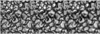 |
Fig. 1 Noiseless quiet-sun region simulated for our numerical experiments. Panel (a) Original (noiseless, diffraction-free, and jitter-free) MHD simulation. (b) Simulated scene after including diffraction effects of the SUNRISE telescope. Panel (c) Degraded scene after including both diffraction effects and jitter with rms amplitudes σx = σy = 0.″1 (∼1.8 px). Ticks are placed every 2.″75. Contrasts are labeled on the upper right corner of each image. Note that both the diffraction effects and jitter significantly decrease the contrast of the simulation. |
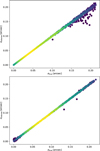 |
Fig. 2 Norm of the inferred jitter amplitude against the simulated (true) one. Top: noiseless case. Bottom: numerical experiment with S/N = 100. There is an almost perfect correlation between the sensed and true jitter amplitudes up to ∼0.″10 when the simulated images are free from noise. The results begin to scatter from there on, with the algorithm tending to underpredict the induced jitter. When noise is included, the algorithm is more stable above 0.″10, but shows more dispersion below∼0.″01. |
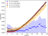 |
Fig. 3 Residual jitter against the time gap between simulated images employed by the algorithm for S/N = 100 and for different levels of induced jitter. The dots represent the mean value of the residual jitter inferred for 100 realizations of the jitter. Errors, estimated as the standard deviation of the results over the 100 realizations, are shown also as a filled area. When jitter is induced in the simulations, the mean values of ∆σ display little sensitivity for time gaps up to ∼10 s, but increase nonlinearly with the time interval above that threshold almost regardless of the jitter amplitude. When the data is free of jitter, the algorithm senses an artificial fluctuating jitter with an amplitude below ∼0.″005 no matter the cadence time employed in the simulation. |
4 Applications to TuMag data
We applied our method to a 35-min time series of images acquired by TuMag that is affected by temporal variations of jitter. This series was recorded on July 14, 2024, from 13:51 to 14:26 UTC while tracking a sunspot. The analyzed images correspond to one modulation state in the continuum of the 525.02 Fe I line, cover an active region of 63″ × 63″ with a 0.″0378 pixel resolution, and have a cadence of ∼30 s. This is the time interval needed to fully complete TuMag’s observation mode #2, which accumulates 16 images per modulation state and wavelength, performs full Stokes vector polarimetry, and samples 8 wavelengths along the spectral line (Del Toro Iniesta et al. 2025). The images were corrected for dark and flat fields and aligned with subpixel accuracy following Guizar-Sicairos et al. (2008).
The selected time series provides a representative test case for the method. It exhibits a wide range of contrast variations, is one of the longest series we have analyzed thus far, and contains diverse solar structures that enable a robust assessment of the reconstruction. These properties make it ideal for demonstrating the expected performance of the algorithm under different observational conditions.
We adopted a sequential approach to sense and correct for time-varying jitter while minimizing the impact of solar evolution. First, we identified the frame of the series with the highest contrast, i, and assumed it to be free of jitter. Next, we used this reference image together with the next frame, i + 1, to minimize Equation (6) and infer the jitter amplitude for the latter. We repeated this process for the previous frame, i − 1. Using these two frames and their inferred OTFs, we determined the jitter affecting the frames i ± 2. This procedure was iterated throughout the series to estimate the jitter amplitude for every frame, ensuring that the time gap between the pairs of images used in the merit function remained ∼30 s.
The assumption that at least one image in the time series is unaffected by jitter is not strictly true, but it represents a reasonable approximation as long as the highest-contrast image is restored well when corrected solely for the WFE sensed through PD. Even if the highest-contrast image were affected by jitter, differential variations could still be estimated and compensated along the series using this method. Indeed, we found that this approach produces a significantly better jitter correction than when sensed jointly for every pair of sequential images along the series, in agreement with the results found for our numerical experiments.
Figure 4 shows the contrast of the images computed over the full FoV and the norm of the sensed jitter, σ, along the series. The contrast fluctuates in the range 14.0%−14.7% with variations from one image to the next that can be as large as ∼0.6 percentage points. Although these fluctuations are not negligible, they are small compared to the contrast variations usually observed in ground instrumentation due to seeing.
The sensed jitter falls in the range 0.″05–0.″15 (∼1–4 px) in most cases and is therefore comparable to the spatial resolution of the instrument (Arroyo Caballero et al. 2025). Based on the results obtained in Section 3, the cadence time of the series, and the amplitude of the inferred jitter, the estimated accuracy of the method is of the order 0.″01, several times better than the observed amplitudes.
Smaller values of contrast are generally related to higher jitter rms values. This is evident in Fig. 5, where the value of the inferred jitter is plotted against the contrast of the original image. The observed anticorrelation suggests that the algorithm tries to compensate the loss of contrast in jittered images by inferring higher values of the rms jitter amplitude, as expected.
We restored the time series from both jitter and the WFE aberrations estimated from a PD calibration recorded very close in time, at 13:07. The inferred WFE rms amplitude amounts to ∼λ/6 including the telescope, the image stabilization, and light distribution system, and the instrument aberrations. We used the modified Wiener filter presented in Martínez Pillet et al. (2011) and tuned the regularization parameter k in its Eq. (15) to 0.05 in order to find a good compromise between noise amplification and contrast of the reconstructed images.
Figure 6 shows the lowest-contrast (LC) and highest-contrast (HC) images of the series before reconstruction (top panels), after correcting for aberrations (middle panels), and after restoring from both wavefront errors and jitter (bottom panels). The temporal evolution of the whole time series before and after WFE and jitter correction is available as an online movie.
The LC and HC images were recorded 5 min 30 s apart (frames 47 and 58 along the series). Although the difference in contrast between them is relatively small before any reconstruction is applied (14% and 14.7%), small-scale features such as filaments or the intergranule network are clearly blurred in the former. When correcting for the inferred WFE, the HC image is much sharper and displays a significantly higher contrast than the LC image (17.9% vs 16%). We ascribe this difference in the restored images to the nonnegligible impact of jitter in the image with lowest contrast, which cannot be corrected just by restoring the wavefront error. After reconstructing both aberrations and the jitter sensed by our method (σx ≃ 0.″09 ≃ 2.4 pixels; σy ≃ 0.″16 ≃ 4.2 pixels), the contrast value for the LC image increases up to 17.5%, very close to the contrast found for the HC image. Filaments and granules also look much sharper. The overall improvement suggests therefore that the inferred OTF is able to correct the effects of jitter in our images, at least to the extent that the contrast of the more strongly jitter-affected images approaches that of the least affected. It is also important to emphasize that this is a worst-case scenario. Most of the images in the time series already exhibit better optical quality and improve significantly when restored solely for static wavefront aberrations.
One limitation of including jitter in the restoration process is that it reduces the amplitude of the modulation transfer function (MTF) – the module of the OTF – at mid- to high-frequencies. In fact, the larger the rms amplitude of the jitter, the narrower the OTF becomes and the lower the effective cut-off frequency of the restored image. Figure 7 shows the azimuthally averaged MTF term of TuMag for different scenarios as a function of the spatial frequency normalized by the critical frequency of the telescope, νc ≡ λD−1, where λ is the operating wavelength of the instrument (525.02 nm) and D is the diameter of the telescope (1 m). We distinguished between the MTF term due to the net effect of the WFE aberrations, as well as the jitter MTF term obtained for the LC image. The “effective” MTF that combines these two effects and an ideal scenario in which no aberrations or jitter are present for a telescope with and without central obscuration of 32.4% is also shown. The combined impact of the central obscuration with the wavefront error and jitter drastically reduces the MTF amplitude of the instrument, especially at mid- to high-frequencies. The MTF for the LC image is virtually zero above ∼0.3νc, thus limiting the reconstruction up to this frequency. Meanwhile, the cut-off for the optimum noise filter for the HC image – unaffected by jitter – is about ∼0.6νc (not shown). Lower cut-off frequencies of the noise filter unavoidably limit the restoration of small-scale details. This is possibly the main reason why the reconstruction of the LC image is still not as good as that of the HC image. However, most of the lost contrast and blurring are compensated for when jitter is taken into account in the restoration.
Figure 8 shows the contrast for the series of restored images over the full FoV. Two cases are shown: (1) where only wavefront aberrations are compensated and (2) where both jitter and the WFE are reconstructed. In the first case, the mean contrast over the full FoV is 17.0%. Its standard deviation along the series is 0.4%. Steep changes in the contrast can be observed from time to time in this case, for example, for frames 25, 32, or 44. Correcting for jitter increases the mean contrast value to 17.7% and decreases the standard deviation to 0.2%.
In other words, the contrast not only improves when correcting for jitter but its fluctuations along the series are damped considerably, even though they are not removed completely. We attribute these residual variations of the contrast primarily to the decrease in the effective cut-off frequency of the power spectrum in restored images as the jitter amplitude increases. Since larger jitter amplitudes limit the amount of detail that can be recovered, contrast in reconstructed images cannot be uniformly restored across the whole series. Indeed, the contrast for the reconstructed data is somehow correlated with that of the original image.
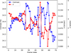 |
Fig. 4 Contrast values of the image (blue dots) and the norm of the inferred jitter (red dots) – both in arcsec and pixel units – along the selected TuMag series. In some cases, fluctuations as large as ∼0.6 percentage points arise from one image to the next. The algorithm systematically compensates for lower contrast values by inferring a larger jitter amplitude. |
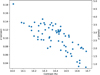 |
Fig. 5 Value of the inferred jitter amplitude in arcsec units (left Y axis) and in pixels units (right Y axis) against the contrast of the original image. The two variables are negatively correlated, as the algorithm tends to assign lower contrasts to data affected by larger jitter. |
5 Summary and conclusions
We present a method that infers the rms amplitude and direction of jitter in solar images whose exposure time is much longer than the typical timescale of the vibrations produced by it. The technique employs only two images of the same scene that are recorded sequentially, under the condition that each of them is affected by a different amount of jitter.
Our method allows for correction of the high-frequency residual jitter left by the telescope image stabilization system. This technique is particularly valuable for time series where the contrast fluctuates between consecutive images due to variations in temporal jitter. The inferred jitter can be employed to correct its impact on the images, thus improving their contrast and reducing the blurring produced by it. The degree of reconstruction is, of course, limited. The higher the sensed jitter amplitude, the lower the effective cut-off frequency of the reconstructed image. This constraint prevents small-scale (high-frequency) details from being recovered in images strongly affected by jitter.
We performed a series of numerical experiments to assess the performance of our method. To this purpose, we employed a dynamical MHD simulation affected by jitter and degraded by the diffraction effects of a critically-sampled 1-m telescope with a central obscuration, similar to SUNRISE III. We also considered two scenarios: that images are free from noise and that they are affected by a noise level of 10−2 with respect to Stokes I at the continuum. Our simulations indicate that the method is extremely robust when neglecting the temporal evolution of the solar scene between the two images, with errors typically below 0.″003 for jitter rms amplitudes as large as 0.″15 in both the X and Y directions and a low signal-to-noise ratio of 100. We also found that the inclusion of random noise in the images helps the algorithm to converge towards the true solution when the induced jitter amplitude along the X and Y directions is above ∼0.″10.
When considering the effect of the temporal evolution of the solar scene, the accuracy of our algorithm is still better than 0.″005 (≲0.1 px) for images recorded less than 10 s apart, rms jitter amplitudes as large as 0.″15 in the X and Y directions, and a worst-case S/N of 100. Even for long time gaps of 30 s between images, the errors found are below 0.″01.
We finally applied our technique to a 35-min time series of modulated images recorded at the continuum of the Fe I 525.02 nm line. The selected images were acquired by the TuMag instrument onboard SUNRISE III and are affected by temporally-changing jitter. The cadence of the chosen datasets is ∼30 s.
We found that the sensed jitter rms amplitudes vary widely within the range 0.″05–0.″15 (∼1–4 px) along the series and are anticorrelated to the contrast of the original (not-corrected) images. Wavefront restoration significantly improves the mean contrast (from 14.3% to 17%) and sharpness of the data. Compensating for the inferred jitter increases the mean contrast in the series of images by an additional 0.7%. In some cases, the contrast improves by as much as 1.5 percentage points – from 16% to 17.5% for the image with the lowest contrast – and its fluctuations are reduced from 0.4% to 0.2% along the time series. These jitter variations represent a worst-case scenario for the TuMag instrument and are much smaller than those usually observed in ground-based solar telescopes.
Although designed for the specific characteristics and constraints of TuMag, the technique may be applied to other imaging spectropolarimeters, provided that their data exhibit measurable contrast variations along a time series. Such fluctuations typically arise when residual high-frequency jitter affects the images differently from one exposure to the next. In instruments where residual jitter is dominated by low-frequency components that vary more slowly than exposure time, our method would offer little or no advantage over standard image alignment techniques. However, for systems in which high-frequency jitter contributes noticeably to contrast degradation, the approach presented here can provide a practical means to estimate and mitigate its impact. Our algorithm is particularly relevant for spaceborne instruments with spatial resolutions below one-tenth of an arcsecond. In these instruments, stability requirements are very demanding and computationally intensive methods, such as MOMFBD, cannot be used to correct jitter-induced wavefront fluctuations in real time.
Under the conditions mentioned above, our algorithm can be applied to any polarimetric modulation state and wavelength along the spectral line of interest. Beyond improving polarization signal amplitude – decreased by the blurring induced by jitter – it can reduce spurious polarimetric signals (“crosstalk”) caused by temporal variations of the jitter. The resulting enhancement in polarimetric sensitivity directly impacts the ability of such instruments to detect small-scale magnetic structures (Bellot Rubio & Orozco Suárez 2019).
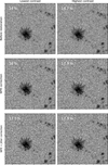 |
Fig. 6 Top: lowest- (LC) and highest-contrast (HC) images along the series before restoration (top left and right panels, respectively). Ticks every 7.″56. Middle: reconstruction after WFE compensation. Bottom: Restoration after WFE and jitter correction. The same color map limits were applied to all images to better compare the enhancement after the different reconstructions. The temporal evolution is available as an online movie. When the effect of jitter is considered, the reconstruction of the LC image improves substantially compared to that obtained with the standard wavefront reconstruction. The contrast is also much closer to that of the nearly jitter-free HC image. |
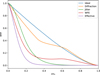 |
Fig. 7 Radial MTF for different scenarios as a function of the frequency (normalized by the critical frequency of the telescope): an ideal 1-m class critically-sampled and aberration-free telescope with no central obscuration (blue), an aberration-free telescope with the 32.4% central obscuration of SUNRISE III (orange), a telescope affected only by the amount of jitter as the one sensed for the lowest-contrast image of Fig. 6 (green), a telescope affected only by the aberrations sensed through PD (red), and a telescope affected both by jitter and aberrations (violet). Compared to an ideal case, the MTF amplitude decreases when introducing wavefront aberrations and/or jitter. The net effect of these two factors effectively reduces the cut-off frequency of the telescope. |
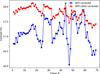 |
Fig. 8 Contrast of the WFE-restored images over the full FoV when jitter correction is applied (red dots) and when not (blue dots). When compensating for jitter, the contrast of the images is increased and its fluctuations are dumped along the series. |
Data availability
Movie associated with Fig. 6 is available at https://www.aanda.org
Acknowledgements
SUNRISE III is supported by funding from the Max Planck Foundation, NASA under Grant #80NSSC18K0934 and #80NSSC24M0024 (“Heliophysics Low Cost Access to Space’ program), and the ISAS/JAXA Small Mission-of-Opportunity program and JSPS KAKENHI JP18H05234/JP23H01220. The Spanish contributions have been funded by the Spanish MCIN/AEI/10.13039/501100011033/ projects RTI2018-096886-B-C5, PID2021-125325OB-C5, CNS2023-144723, and from “Center of Excellence Severo Ochoa” awards to IAA-CSIC (SEV-2017-0709, CEX2021-001131-S), all co-funded by European REDEF funds, “A way of making Europe”. This research has received financial support from the European Union’s Horizon 2020 research and innovation program under grant agreement No. 824135 (SOLARNET) and No. 101097844 (WINSUN)from the European Research Council (ERC). It has also been funded by the Deutsches Zentrum für Luft-und Raumfahrt e.V. (DLR, grant no. 50 OO 1608). The contributions of E. Harnes have been supported by the International Max Planck Research School (IMPRS) for Solar System Science at the University of Göttingen, Germany. J.C. Trelles Arjona and C. Kuckein acknowledge financial support from project PID2024-156066OB-C55. C. Kuckein also acknowledges grant RYC2022-037660-I funded by MCIN/AEI/10.13039/501100011033 and by “ESF Investing in your future”.
References
- Arroyo Caballero, D., Del Toro Iniesta, J. C., Bailén, F. J., et al. 2025, A&A, submitted [Google Scholar]
- Bailén, F. J., Orozco Suárez, D., Blanco Rodríguez, J., et al. 2022a, ApJS, 263, 7 [Google Scholar]
- Bailén, F. J., Orozco Suárez, D., Blanco Rodríguez, J., et al. 2022b, ApJS, 263, 8 [Google Scholar]
- Barthol, P., Gandorfer, A., Solanki, S. K., et al. 2011, Sol. Phys., 268, 1 [Google Scholar]
- Bellot Rubio, L., & Orozco Suárez, D. 2019, Liv. Rev. Sol. Phys., 16, 1 [Google Scholar]
- Berkefeld, T., Bell, A., Volkmer, R. et al. 2025, Sol. Phys., 300 [Google Scholar]
- Bernasconi, P., Carpenter, M., Eaton, H., et al. 2025, Sol. Phys., 300, 112 [Google Scholar]
- Born, M., & Wolf, E. 1999, Principles of Optics, by Max Born and Emil Wolf (Cambridge, UK: Cambridge University Press), 986 [Google Scholar]
- Del Toro Iniesta, J. C., & Martínez Pillet, V. 2012, ApJS, 201, 22 [CrossRef] [Google Scholar]
- Del Toro Iniesta, J. C., Orozco Suárez, D., Álvarez-Herrero, A., et al. 2025, Sol. Phys., 300, 148 [Google Scholar]
- Feller, A., Gandorfer, A., Grauf, B., et al. 2025, Sol. Phys., 300, 65 [Google Scholar]
- Fiete, R. D., & Paul, B. D. 2014, Opt. Eng., 53, 1 [Google Scholar]
- Gonsalves, R. A., & Chidlaw, R. 1979, Proc. SPIE, 207, 32 [NASA ADS] [CrossRef] [Google Scholar]
- Guizar-Sicairos, M., Thurman, S. T., & Fienup, J. R. 2008, Opt. Lett., 33, 156 [NASA ADS] [CrossRef] [Google Scholar]
- Iglesias, F. A., Feller, A., Gandorfer, A., et al. 2025, Sol. Phys., 300, 58 [Google Scholar]
- Johnson, J. F. 1993, Appl. Opt., 32, 6503 [Google Scholar]
- Katsukawa, Y., et al. 2025, Sol. Phys., 300 [Google Scholar]
- Korpi-Lagg, A., Gandorfer, A., Solanki, S. K., et al. 2025, Sol. Phys., 300, 75 [Google Scholar]
- Löfdahl, M. G., & Scharmer, G. B. 1994, A&AS, 107, 243 [NASA ADS] [Google Scholar]
- Martínez Pillet, V., Del Toro Iniesta, J. C., Álvarez-Herrero, A., et al. 2011, Sol. Phys., 268, 57 [Google Scholar]
- Paxman, R. G., Schulz, T. J., & Fienup, J. R. 1992, J. Opt. Soc. Am. A, 9, 1072 [CrossRef] [Google Scholar]
- Pittelkau, M. E., & McKinley, W. G. 2016, Opt. Eng., 55, 063108 [Google Scholar]
- Solanki, S. K., Barthol, P., Danilovic, S., et al. 2010, ApJ, 723, L127 [NASA ADS] [CrossRef] [Google Scholar]
- Solanki, S. K., Riethmüller, T. L., Barthol, P., et al. 2017, ApJS, 229, 2 [NASA ADS] [CrossRef] [Google Scholar]
- van Noort, M., Rouppe van der Voort, L., & Löfdahl, M. G. 2005, Sol. Phys., 228, 191 [Google Scholar]
- Vögler, A., Shelyag, S., Schüssler, M., et al. 2005, A&A, 429, 335 [Google Scholar]
All Figures
|
Fig. 1 Noiseless quiet-sun region simulated for our numerical experiments. Panel (a) Original (noiseless, diffraction-free, and jitter-free) MHD simulation. (b) Simulated scene after including diffraction effects of the SUNRISE telescope. Panel (c) Degraded scene after including both diffraction effects and jitter with rms amplitudes σx = σy = 0.″1 (∼1.8 px). Ticks are placed every 2.″75. Contrasts are labeled on the upper right corner of each image. Note that both the diffraction effects and jitter significantly decrease the contrast of the simulation. |
| In the text | |
|
Fig. 2 Norm of the inferred jitter amplitude against the simulated (true) one. Top: noiseless case. Bottom: numerical experiment with S/N = 100. There is an almost perfect correlation between the sensed and true jitter amplitudes up to ∼0.″10 when the simulated images are free from noise. The results begin to scatter from there on, with the algorithm tending to underpredict the induced jitter. When noise is included, the algorithm is more stable above 0.″10, but shows more dispersion below∼0.″01. |
| In the text | |
|
Fig. 3 Residual jitter against the time gap between simulated images employed by the algorithm for S/N = 100 and for different levels of induced jitter. The dots represent the mean value of the residual jitter inferred for 100 realizations of the jitter. Errors, estimated as the standard deviation of the results over the 100 realizations, are shown also as a filled area. When jitter is induced in the simulations, the mean values of ∆σ display little sensitivity for time gaps up to ∼10 s, but increase nonlinearly with the time interval above that threshold almost regardless of the jitter amplitude. When the data is free of jitter, the algorithm senses an artificial fluctuating jitter with an amplitude below ∼0.″005 no matter the cadence time employed in the simulation. |
| In the text | |
|
Fig. 4 Contrast values of the image (blue dots) and the norm of the inferred jitter (red dots) – both in arcsec and pixel units – along the selected TuMag series. In some cases, fluctuations as large as ∼0.6 percentage points arise from one image to the next. The algorithm systematically compensates for lower contrast values by inferring a larger jitter amplitude. |
| In the text | |
|
Fig. 5 Value of the inferred jitter amplitude in arcsec units (left Y axis) and in pixels units (right Y axis) against the contrast of the original image. The two variables are negatively correlated, as the algorithm tends to assign lower contrasts to data affected by larger jitter. |
| In the text | |
|
Fig. 6 Top: lowest- (LC) and highest-contrast (HC) images along the series before restoration (top left and right panels, respectively). Ticks every 7.″56. Middle: reconstruction after WFE compensation. Bottom: Restoration after WFE and jitter correction. The same color map limits were applied to all images to better compare the enhancement after the different reconstructions. The temporal evolution is available as an online movie. When the effect of jitter is considered, the reconstruction of the LC image improves substantially compared to that obtained with the standard wavefront reconstruction. The contrast is also much closer to that of the nearly jitter-free HC image. |
| In the text | |
|
Fig. 7 Radial MTF for different scenarios as a function of the frequency (normalized by the critical frequency of the telescope): an ideal 1-m class critically-sampled and aberration-free telescope with no central obscuration (blue), an aberration-free telescope with the 32.4% central obscuration of SUNRISE III (orange), a telescope affected only by the amount of jitter as the one sensed for the lowest-contrast image of Fig. 6 (green), a telescope affected only by the aberrations sensed through PD (red), and a telescope affected both by jitter and aberrations (violet). Compared to an ideal case, the MTF amplitude decreases when introducing wavefront aberrations and/or jitter. The net effect of these two factors effectively reduces the cut-off frequency of the telescope. |
| In the text | |
|
Fig. 8 Contrast of the WFE-restored images over the full FoV when jitter correction is applied (red dots) and when not (blue dots). When compensating for jitter, the contrast of the images is increased and its fluctuations are dumped along the series. |
| In the text | |
Current usage metrics show cumulative count of Article Views (full-text article views including HTML views, PDF and ePub downloads, according to the available data) and Abstracts Views on Vision4Press platform.
Data correspond to usage on the plateform after 2015. The current usage metrics is available 48-96 hours after online publication and is updated daily on week days.
Initial download of the metrics may take a while.