| Issue |
A&A
Volume 708, April 2026
|
|
|---|---|---|
| Article Number | A239 | |
| Number of page(s) | 10 | |
| Section | Astronomical instrumentation | |
| DOI | https://doi.org/10.1051/0004-6361/202558510 | |
| Published online | 09 April 2026 | |
The VLT/ERIS grating vector Apodizing Phase Plate coronagraph
Design and on-sky performance
1
Leiden Observatory, Leiden University,
Postbus 9513,
2300 RA
Leiden,
The Netherlands
2
ETH Zurich, Institute for Particle Physics & Astrophysics,
Wolfgang-Pauli-Str. 27,
8093
Zurich,
Switzerland
3
SRON Netherlands Institute for Space Research,
Niels Bohrweg 4,
2333 CA,
Leiden,
The Netherlands
4
Institute for Astronomy, University of Edinburgh, Royal Observatory,
Blackford Hill,
Edinburgh
EH9 3HJ,
UK
5
European Southern Observatory,
Karl-Schwarzschild-Straße 2,
85748
Garching bei München,
Germany
6
Max Planck Institute for Intelligent Systems,
Max-Planck-Ring 4,
72076
Tübingen,
Germany
7
ETH Zurich, Department of Earth and Planetary Sciences,
Sonneggstrasse 5,
8092
Zurich,
Switzerland
8
National Solar Observatory,
3665 Discovery Dr.,
Boulder,
Co
80303,
USA
9
STAR Institute, Université de Liège,
Allée du Six Août 19c,
4000
Liège,
Belgium
10
European Southern Observatory,
Alonso de Córdova 3107, Vitacura, Casilla
19001,
Santiago,
Chile
11
School of Natural Sciences, Center for Astronomy, University of Galway,
Galway
H91 CF50,
Ireland
12
Instituto de Estudios Astrofísicos, Facultad de Ingeniería y Ciencias, Universidad Diego Portales,
Av. Ejército Libertador 441,
Santiago,
Chile
13
Millennium Nucleus on Young Exoplanets and their Moons (YEMS),
Chile
14
Astrophysics, University of Oxford,
Denys Wilkinson Building, Keble Road,
Oxford
OX1 3RH,
UK
15
INAF – Osservatorio Astronomico di Padova,
Vicolo dell’Osservatorio 5,
35122,
Padova,
Italy
16
Physikalisches Institut, Universität zu Köln,
Zülpicher Str. 77,
50937,
Köln,
Germany
17
Max-Planck-Institut für extraterrestrische Physik,
Postfach 1312,
85741,
Garching,
Germany
18
INAF – Osservatorio Astronomico d’Abruzzo,
Via Mentore Maggini,
64100,
Teramo,
Italy
19
INAF – Osservatorio Astrofisico di Arcetri,
largo E. Fermi 5,
50125
Firenze,
Italy
20
STFC UK ATC, Royal Observatory Edinburgh,
Blackford Hill. Edinburgh
EH9 3HJ,
UK
★ Corresponding author: This email address is being protected from spambots. You need JavaScript enabled to view it.
Received:
10
December
2025
Accepted:
6
March
2026
Abstract
Aims. We describe the design, laboratory manufacture, and on-sky testing of the grating vector apodizing phase plate (gvAPP) coronagraph for the Enhanced Resolution Imager and Spectrograph (ERIS) on the Very Large Telescope.
Methods. We used both laboratory measurements and on-sky observations to characterise the gvAPP in several different filters, from the K to the L band.
Results. In testing, the gvAPP reaches its design specification in the transmission of the optic with 90% in the K bands and 60% in the L band. While the gvAPP reaches its designed raw contrast performance of 1 × 10⁻⁵, it does not reach the post-processed contrast of 5 × 10⁻⁵ in on-sky observations. Electronic detector noise, due to the Airy core of the coronagraphic point spread function inducing cross-talk between the readout amplifiers, produces a repeated pattern within the coronagraphic regions of the gvAPP.
Conclusions. Despite these limitations, we recommend the gvAPP as a tool for characterising substellar companions with known separations and position angles, which allow them to be placed in the coronagraphic dark holes for observations. The ERIS gvAPP’s leakage term can also be used as a photometric reference for time series observations; however, we caution that the contrast performance may limit such studies to only the brightest targets. ERIS gvAPP data quality may be improved further with better modelling of detector electronic noise. This work is a pathfinder for Extremely Large Telescope instruments including METIS, which will include gvAPP coronagraphs with improved designs based on these results.
Key words: instrumentation: high angular resolution
F.R.S.-FNRS Research Director.
© The Authors 2026
 Open Access article, published by EDP Sciences, under the terms of the Creative Commons Attribution License (https://creativecommons.org/licenses/by/4.0), which permits unrestricted use, distribution, and reproduction in any medium, provided the original work is properly cited.
This article is published in open access under the Subscribe to Open model. This email address is being protected from spambots. You need JavaScript enabled to view it. to support open access publication.
1 Introduction
The Enhanced Resolution Imager and Spectrograph (ERIS; Davies et al. 2023) is a diffraction-limited imager and spectrograph for the Very Large Telescope (VLT). It is composed of two parts, the integral field spectrograph SPIFFIER (George et al. 2016) and a diffraction-limited 1 to 5 micron high-angular-resolution imager, the Near Infrared Camera System (NIX; Pearson et al. 2016), which has two pixel scales (13 mas covering 26.4″ × 26.4″ and 27 mas covering 55.4″ × 55.4″). The science goals of ERIS include the detection and characterisation of extrasolar planets and circumstellar disks around bright stars (e.g. Maio et al. 2025).
The diffraction halo of the central star overwhelms the signals from objects adjacent to the star, making studies of these sources difficult to impossible. Coronagraphs are angular filters – they suppress the wavefront from point-like sources on the sky whilst simultaneously allowing wavefronts from adjacent astrophysical sources to pass through to the science camera focal plane (see Kenworthy & Haffert 2025 for a review). Focal-plane coronagraphs use a combination of amplitude and phase modifications so that the propagated starlight in the subsequent pupil plane can be blocked by an appropriately matched mask. Pupil-plane coronagraphs achieve this goal by modifying the wavefront in the pupil plane to redistribute the diffraction structure of the point spread function (PSF) in the science camera focal plane. At infrared wavelengths, these coronagraphs have the advantage that the stellar suppression is independent of chopping and telescope pointing. In addition, the flux of the rearranged starlight makes image alignment easier in post-processing. The ERIS NIX instrument is equipped with two coronagraphs, a grating vector-apodized pupil plane coronagraph (Otten et al. 2017) and a vector vortex coronagraph (Orban de Xivry et al. 2024).
The apodizing phase plate (APP; Codona & Angel 2004) adds a specific phase pattern in the telescope pupil without changing the amplitude of the electric field. This phase pattern modifies the PSF of the instrument and suppresses diffraction structures in a 180-degree-wide semi-circular region next to a target star, referred to as a ‘dark hole’ (see Fig. 1). This is demonstrated on-sky in Kenworthy et al. (2007) using the variation in thickness of a ZnSe substrate to induce the designed phase pattern at one central wavelength using an APP coronagraph (Kenworthy et al. 2010) with NAOS/CONICA (Lenzen et al. 2003; Rousset et al. 2003); this resulted in the characterisation of Beta Pictoris b (Quanz et al. 2010) and the discovery of the substellar companion HD 100546b (Quanz et al. 2013). The original implementation of the APP does not work for broader bandwidths due to the chromatic nature of available substrates. An alternative approach provides the ability to make phase-based coronagraphs achromatic over much wider bandwidths: by using the geometric phase (the Pancharatnam-Berry phase; Pancharatnam 1956; Berry 1984), almost any phase pattern can be encoded in the orientation of the fast axis of an optically active polymer.
Unpolarised light can be decomposed into equal amounts of left and right circularly polarised light, and the vast majority of stars and planets emit almost completely unpolarised light. Using the geometric phase, both circular polarisations will have the phase pattern encoded in them, but with opposite signs of the given phase pattern. The 180◦ dark hole phase pattern is anti-symmetric, which means that the dark hole will be symmetrically point-flipped to the opposite side of the star, thereby providing full dark hole azimuthal coverage around the star. A quarter-wave plate and Wollaston prism placed after the optically active polymer then splits the two opposite circularly polarised beams towards different locations in the focal plane (Otten et al. 2014), separating the two coronagraphic PSFs (e.g. Fig. 1, right panel). A single layer of a given polymer is highly chromatic, but combining several carefully specified layers with different chromatic properties, each of which self-align with the layer beneath it, allows achromaticity to be generated over an octave in bandwidth, resulting in a vector apodizing phase plate (vAPP; Snik et al. 2012). The addition of a sinusoidally periodic phase ramp into the phase pattern generates a polarisation diffraction grating in the pupil beam. This diffracts the two circular polarisations into the m = ±1 orders, separating them at the focal plane and removing the need for the Wollaston prism and quarter-wave plate: this is the principle behind the grating vector apodizing phase plate (gvAPP; Otten et al. 2017). There are now gvAPP coronagraphs installed at telescopes worldwide, enabling a range of scientific goals: searches for directly imaged exoplanets (Long et al. 2018, 2023; Barbato et al. 2025; Mesa et al. 2025), the spectroscopic characterisation of known substellar companions, including the HR 8799 exoplanets (Sutlieff et al. 2021; Doelman et al. 2022), imaging of the protoplanetary disk around PDS 201 (Wagner et al. 2020), variability monitoring of the substellar companion HD 1160 B (Sutlieff et al. 2023, 2024), and the development of focal-plane wavefront sensing and spatial linear dark field control (Bos et al. 2019; Miller et al. 2019, 2021). An overview of existing and upcoming gvAPP coronagraphs is found in Doelman et al. (2021).
In this paper, we report on the theoretical, laboratory, and on-sky performance of the gvAPP coronagraph in the ERIS NIX instrument. We discuss the phase pattern design, construction, and cryogenic testing in Sect. 2. We then describe the on-sky measurements, including PSF validation and the attained contrast curves, in Sect. 3, before analysing the performance of the gvAPP and making recommendations for its use in Sect. 4. Finally, we highlight our conclusions in Sect. 5.
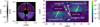 |
Fig. 1 ERIS gvAPP phase pattern design and simulated PSF. Left: phase within the defined gvAPP pupil. Right: resultant three PSFs of the gvAPP. We show the two coronagraphic PSFs and the central leakage term. Three astrometric reference spots can be seen. The scale is logarithmic in normalised intensity. |
2 Design and construction
2.1 Optical design
We used a gvAPP design algorithm that can find dark hole solutions for arbitrarily shaped telescope pupils and dark hole geometries (Doelman et al. 2021). We took the ERIS pupil geometry to be the VLT primary mirror, secondary support structure, and secondary mirror, with a rectangular extension next to the secondary mirror caused by the tertiary mirror raised up into its stow position (see Fig. 1, left panel). A thin metal mask (the ‘amplitude mask’) in the gvAPP both defines the pupil for the coronagraph and acts as a cold stop, preventing thermal emission from the telescope support structures reaching the science camera focal plane.
In order for the gvAPP pupil to be fully illuminated by the telescope pupil within ERIS (which is subject to flexure and alignment tolerances), the gvAPP optic is undersized (d = 11.50 mm) with respect to the nominal diameter of the reimaged ERIS pupil (d = 11.76 mm). The design parameters are listed in Table 1.
In monochromatic light, the gvAPP produces three PSFs. Two of these are coronagraphic PSFs with a dark hole on one side of the PSF Airy core of the target star, matching the PSF of the gvAPP pupil phase pattern (see Fig. 1). These two PSFs are displaced by equal distances on either side of a central leakage term PSF, which corresponds to the PSF of the amplitude mask alone (i.e. an unmodified PSF of the target star at a fraction of its original flux). The majority of the stellar flux is divided equally between the two coronagraphic PSFs, and a small fraction remains in the leakage term PSF. The ERIS gvAPP design has two additional faint PSFs that are added perpendicular to the coronagraphic PSF separation axis – these act as astrometric references to align the images if the cores of the coronagraphic PSFs are over-saturated. A diffraction grating pattern is added to the vAPP phase pattern: this diffraction grating of 25 cycles across the gvAPP pupil means that the separation between the coronagraphic PSFs are separated 25λ/D from the leakage PSF, and a similar effect occurs for the astrometric reference PSFs. Since the location of the coronagraphic PSFs (and any associated faint companion next to the star) scales with wavelength, any faint companions that are in one of the dark holes will have smearing along a line between the companion and leakage PSF. Thus, although the gvAPP can work at all wavelengths accessible to ERIS, to avoid excessive smearing, the gvAPP should only be used with narrow band filters with a maximum fractional bandwidth of 6% (Dubber et al. 2022).
Two gvAPPs have been manufactured by ImagineOptix in 2018, and the best gvAPP chosen based on the transmission in the operating wavelength range. The manufacturing method of the patterned liquid-crystal layers is identical to the MagAO gvAPP (Otten et al. 2017) and is described in detail in Kim et al. (2015). Here, we outline the optical assembly unique to the ERIS gvAPP.
The gvAPP consists of four individual CaF2 substrates glued together. Four substrates are required due to two manufacturing limitations. First, the anti-reflection (AR) coating cannot be applied to the opposite side of the substrate of the amplitude mask, resulting in the need for a separate AR-coated substrate of 1 mm thickness. Second, it is not possible to apply the liquid-crystal film to the wedged substrate because of the wedge angle of 0.44 degrees. The four substrates have a total thickness of 7.55 mm at the thick end of the wedge (7.39 mm at the thin end of the wedge) with an overall measured diameter of 20.95 mm. The substrates are glued together with NOA-61 and aged 10 hrs at 50◦C. The slope of the wedge is perpendicular to the line of the three PSFs and chosen to prevent reflection ghosts from the coronagraphic PSFs appearing in the gvAPP corona-graphic holes. The amplitude mask is made of aluminium with a thickness ∼300 nm. We confirmed that the centre of the clear aperture of the mask is 0.020 mm from the centre of the 21 mm substrates. The AR coatings have <0.5% average reflectance each. ImagineOptix report an alignment error of <1 micron between the centre of the liquid-crystal pattern and the centre of the aluminium mask, although this was not independently verified.
Design parameters for the ERIS gvAPP including the inner working angle (IWA) and outer working angle (OWA).
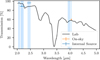 |
Fig. 2 Optical transmission of the gvAPP measured in the laboratory (black curve) and the on-sky background transmission in the Br-α filter (orange point). Additional measurements with the ERIS internal calibration unit are shown by the blue points. The blue regions trace all filters available for observations with the gvAPP in ERIS. Note that for on-sky throughput, this transmission curve should be multiplied by 0.23 to account for the EE and division of the flux between coronagraphic PSFs (see Sect. 3.2). |
2.2 Optical throughput of the gvAPP
The ERIS gvAPP transmission (measured by ImagineOptix) is shown in Fig. 2 and is measured in a clear aperture portion of the gvAPP using a Thorlabs OSA205 Fourier spectrometer. The measurement includes all substrates, glue layers, liquid crystal polymer (LCP) layer, and AR coatings. The overall transmission in is ∼90% in the K band, ∼50% in the L band, and ∼40% in the M band. The transmission curve is comparable to the Large Binocular Telescope (LBT) double-grating vAPP (dgvAPP) transmission curve found in Doelman et al. (2022). Like the LBT dgvAPP, the absorption feature at 3.3 µm goes to 0% transmission, rendering L-short observations ineffective. This absorption feature is caused by absorption in both the glue and liquid-crystal layers due to vibrational modes of chemical bonds with carbon atoms (Otten et al. 2017).
To verify the transmission in the K band, we used the ERIS internal calibration unit to image the PSFs both with and without the gvAPP in Br-γ, K-peak, IB-2.42, and IB-2.48 filters at two different positions on the detector1. We subtracted the background and used aperture photometry on the PSF cores to obtain the fluxes of the PSFs, including both coronagraphic PSFs and the leakage PSF. The encircled energy (EE) of the Airy core of the coronagraphic APP PSFs is reduced due to the nature of the pupil apodisation. The APP design is a trade-off between coronagraphic suppression and EE fraction. This is calculated by simulating the non-coronagraphic PSF in addition to the APP PSF using
HCIPy(Por et al. 2018) and performing aperture photometry enclosing the central Airy core to the first minimum. We calculated the correction for the undersized pupil using archival pupil images and comparing the area of these pupils on the detector. The phase apodisation reduces the EE transmission to 47.6% and the undersizing of the pupil has a relative transmission of 80% compared to no pupil mask. We divided out these factors to calculate the transmission of the APP optic from the fluxes from the aperture photometry, as shown in Fig. 2.
Observing log.
3 On-sky measurements
The on-sky performance of the ERIS gvAPP in the narrow K- and L-band filters was evaluated in 2022 and 2023; see Table 2 for observing details. The Br-γ, Br-α-cont, and Br-α filters were tested as part of the instrument commissioning, whereas K-peak observations were obtained as part of an open time programme with ESO programme 112.25QA.001 (PI: Sutlieff). We report on the high-contrast imaging performance using the metrics suggested in the Optimal Optical Coronagraph Workshop (Ruane et al. 2018), namely the off-axis throughput, the raw contrast, and the post-processed detection limits in the companion-to-star flux ratio.
3.1 Pre-processing
The features of the gvAPP PSF – in particular the lack of rotational symmetry – render the pre-processing challenging. The following describes the data processing pipeline that is used to convert the raw detector integrations to science-ready images. We used the Python package
pynpoint(Amara & Quanz 2012; Stolker et al. 2019) to reduce all datasets except for the K-peak dataset, which is described in Sect. 3.5.
The first part of the reduction is similar to any adaptive optics (AO) observation taken without a coronagraph. To correct the cosmetics of the detector, the science frames are dark and flat corrected, and then bad pixels are identified via sigma-clipping on the dark and flat frames (as well as in the raw science images) and are replaced by the median of the neighbouring pixels. All our observations follow an ‘AB’ nodding sequence with a telescope offset every 3–5 min in order to subtract the near-IR sky and telescope background. We refer to the two positions on the detector as Nod A and Nod B. We subtracted the sky background at a given nodding position by taking the average of the frames at the opposite nodding position before and after the current position. We subtracted the median of every row and column of the image to remove the remaining detector artefacts presenting as stripes in the image. The science frames were then aligned using cross-correlation, centred using a Gaussian fit to the leakage term PSF, and cropped to include the whole gvAPP PSF pattern. For fainter targets, this alignment was done on the coronagraphic PSFs, as their cores are not saturated. Bad frames during which the AO loop was open were identified by computing the mean-square error of the leakage term PSF relative to the mean science image. The second part of the reduction is specific to gvAPP observations and aims at cutting and stitching together the dark holes of the two coronagraphic PSFs. Since the centres of the coronagraphic PSFs are saturated and are therefore challenging to precisely determine, we identified their position relative to the three astrometric PSFs on the simulated PSF (see Fig. 1). We measured the position of the three central astrometric spots in the science frames and inferred the position of the centres of the coronagraphic PSFs. We then cut out a D-shaped dark hole from each coronagraphic PSF and put them into a single frame. The straight edge of the dark hole lies along the transition between the bright and dark part of the PSF and is offset by 0.5 λ/D, and so in the combined frame we are missing a 1 λ/D wide strip, resulting in incomplete coverage around the central star (see Fig. 3). This pre-processing pipeline delivers science frames containing the two dark holes of the coronagraphic PSFs stitched together, with the 1 λ/D strip parallel to the long side of the ‘D’ masked out.
3.2 Throughput
Contrary to focal plane coronagraphs, to first order, the throughput does not depend on the position of the source in the field of view, as the gvAPP only modifies the wavefront in the pupil plane. This means that the off-axis throughput affecting a companion can be approximated by the transmission of the gvAPP element at the respective wavelength. As described in Sect. 2, the transmission of the gvAPP is measured using a fibre-coupled IR light source and Fourier spectrometer (see Fig. 2). While the K-band transmission of the gvAPP can be measured using the internal calibration unit (see Sect. 2.2), its wavelength limitations mean that the L- and M-band transmission can only be measured on-sky. A differential infrared background measurement is especially suitable to derive the transmission. Two consecutive observations are performed with identical detector integration times (DITs) using the Br-α filter, one with the gvAPP mask in the aperture and one with a mask blocking only the outer telescope support structure. After dark-subtracting the data, we measured the total counts in a region on the detector with no sources and only a few bad pixels. Accounting for the different outer aperture sizes of the gvAPP (12 mm) and the LM-pupil mask in ERIS (11.2 mm), the ratio of the total counts yields a transmission of (59.5 ± 2.2)% in the Br-α filter. While this on-sky measurement of the transmission agrees with the laboratory measurements, we note that it is slightly conservative as it does not account for the additional thermal contribution from the unobstructed spiders when observing with the LM-pupil mask.
The point source throughput with the gvAPP is multiplied by a factor of 0.45 to account for the division between the two coronagraphic PSFs and leakage term, and multiplied by an additional factor of 0.51 for the EE of the Airy cores. This results in a total throughput of 13.6% in the Br-α filter and a throughput of 21.8% for the K-peak filter.
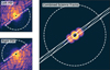 |
Fig. 3 Geometry of combining the two coronagraphic PSFs to form the coverage around the target star. The hatched area is masked out during subsequent image combination and processing. The semi-circular dashed lines are a visual aid only; the area at wider separations beyond these circles is not masked in the combined image. |
3.3 Raw contrast
The raw contrast is evaluated on the HR 8799 dataset in the Br-α-cont filter (see Table 2), which is pre-processed as described in Sect. 3.1. To derive the raw contrast as described in Ruane et al. (2018), this dataset contains the host star as a single bright point source, which produces a high-S/N image of the gvAPP coronagraphic PSF, PSFcoro. This PSF is sampled in apertures AP of diameter λ/D, starting at the coronagraphic PSF core ηs = ∫AP(0) PSFcoro(x) dx and at various places in the dark hole yielding  . The raw contrast is then reported as C(x0) = ηp(x0)/ηs. As the cores of the PSF are saturated in the science images, the raw contrast is calibrated using the unsaturated PSF in the PSF calibration images or can be calibrated using the leakage PSF measurements. To do so, first the raw contrast is calculated in both the science and in a shorter exposure unsaturated coronagraphic PSF image. The science data raw contrast curve is then scaled to match the PSF reference curve in the unsaturated and high-S/N region from 1.5–2 λ/D. As can be seen in Fig. 4, the deepest raw contrast is reached when evaluated perpendicularly to the main axis of the corona-graphic PSF. In this case, the on-sky raw contrast performance in the L band closely follows the laboratory measurement (Boehle et al. 2021) out to about 8 λ/D.
The gvAPP is designed to provide high-contrast in 90% of the region between 2.2 and 15λ/D via its two dark holes. It is therefore instructive to evaluate the raw contrast throughput along the extent of the dark hole. This is done by placing circular apertures of diameter 1 λ/D out to a maximum opening angle of 81◦ perpendicular to the PSF main axis (i.e. the axis perpendicular to the edge of the dark hole, passing through the coronagraphic PSF core). We find that between 4 and 15 λ/D, the raw contrast does not significantly change out to 60◦ away from the perpendicular, allowing for a ∼70% sky access at full raw contrast performance. Beyond 60◦ up to the designed maximum angle of 81◦, the raw contrast starts to be impacted by apertures that partially overlap with the bright side of the coronagraphic PSF. In these regions, full contrast performance is only available from 10 to 15 λ/D.
The median raw contrast performance at ±10◦ to the perpendicular is measured to 1.6 × 10⁻³ at 2.2 λ/D and to an upper limit of 5.3 × 10⁻⁵ at 15 λ/D. Compared to the design parameters in Table 1, this means that the gvAPP underperforms by more than an order of magnitude at the inner working angle (IWA). An analysis by Boehle et al. (2021) shows that polishing errors (with spatial frequencies following a power law) in the reimaging optics can result in a scattered light halo that is consistent with this reduced performance. Microscope measurements show that the manufactured LCP pattern is not the cause of this decrease in raw contrast. At the outer working angle (OWA), the designed contrast performance lies below the sky background limit and cannot be verified on-sky without a longer on-sky integration or a brighter target star.
3.4 Post-processed contrast: Narrow-band filters
To characterise the post-processed detection limits of the ERIS gvAPP in the narrow K and L bands, the stars γ Gru (K = 3.45 mag), HR 8799 (K = 5.24 mag, L = 5.23 mag), and ι Cap (L = 2.18 mag) were observed using the Br-γ, Br-α, and Br-α-continuum filters during commissioning. All three observations follow the same sequence in pupil-tracking mode, to profit from angular differential imaging (ADI) post-processing (Marois et al. 2006). We first recorded a PSF reference using a DIT short enough to avoid any saturation of the gvAPP PSF. For the main observing sequence, the DIT is increased such that the two main gvAPP PSF features are saturated but the central leakage term remains unsaturated. Every 3 min, the star is nodded by 8″ from Nod A to Nod B to estimate and remove the near-IR background. Every DIT is written out in cube mode. The short observation time in Br-α sequence result in a very small field rotation, and the weather conditions were worse than average, resulting in several poor-quality and open AO loop frames within each data cube, which are removed. After pre-processing the data as described in Sect. 3.1, the data are post-processed using principal component analysis (PCA)/ADI (Amara & Quanz 2012). We calculated the detection limits for each filter by performing fake planet injection tests using
applefy(Bonse et al. 2023). The fake planet templates were constructed from the central leakage term of the unsaturated PSF reference and were normalised to match the flux of the coronagraphic PSF using the unsaturated coronagraphic PSF reference image. The contrast curves were then created by selecting the principal component resulting in the deepest contrast at each angular separation (i.e. optimal PCA/ADI; Meshkat et al. 2014) with the bright 1 λ/D strip masked out in subsequent calculations.
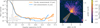 |
Fig. 4 Raw contrast of the gvAPP in the Br-α-continuum filter. Left: raw flux contrast evaluated in λ/D-sized apertures placed in the dark hole over an aperture placed on the PSF centre in the left lobe of a deep integration on HR 8799 at 3.96 µm. The orange line traces the median contrast evaluated in a ±10◦ region perpendicular to the main axis of the gvAPP PSF. The orange markers indicate the IWA and OWA provided in Table 1. The blue curve displays the raw contrast measured on the gvAPP element under laboratory conditions at 2 µm by Boehle et al. (2021) – the values from 10 to 12.5 λ/D are below the sensitivity of the test bench. The rise seen at 13.5 λ/D in the laboratory data is due to limitations from internal reflections in the test bench not present in ERIS. Right: focal plane image of the left lobe of the gvAPP on which the raw contrast was evaluated. The shaded orange wedge is the ±10◦ region in which the orange contrast curve was measured. |
3.5 Post-processed contrast: K-peak filter
The deepest set of observations are 189 min of data taken in the K-peak filter (ESO programme 112.25QA.001, PI: Sutlieff), which has a bandwidth of 0.10 µm. The median airmass, seeing, and coherence time τ for the observations obtained with the K-peak filter (which was designed by Dubber et al. 2022) are given in Table 2. The data were reduced by adapting the method applied by Sutlieff et al. (2021) to MagAO vAPP data. The bad pixel correction was carried out using the ESO’s ERIS-NIX bad pixel map2. An averaged dark frame was created by taking the median of five dark frames, which was then subtracted from every frame in the data. We flat-fielded the data by dividing every frame by a flat frame obtained with the same window size as the data, which we normalised by dividing it by the median value in a region clear of large bad pixel clusters. Background subtraction was carried out using the frames from the opposite nod position. To reduce the computational time, every 360 frames were binned, which resulted in 63 frames per nodding position. We aligned the frames using the
phase_cross_correlationfunction included in the
scikit-image(van der Walt et al. 2014) Python package. We then corrected for row and column systematics by subtracting the median values along each axis, as calculated with the gvAPP PSFs masked. We applied the temporal reference analysis of planets (TRAP; Samland et al. 2021) model to the binned dataset following the optimised method for gvAPP coronagraphic datasets demonstrated in Liu et al. (2023). There are four sub-datasets: each nodding position contains left and right complementary coronagraphic images (e.g. see Fig. 6). We reduced the four sub-datasets independently by taking the stellar PSF in each frame as the PSF model for that frame and selected reference pixels from both the bright and dark sides to build noise models. We derived a contrast map and an unnormalised uncertainty map for each sub-dataset. We combined the contrast maps and uncertainty maps weighted by the uncertainty, firstly for the left and right coronagraphic datasets and secondly for the two nodding positions. The normalisation factor for the final uncertainty was calculated from the combined contrast map divided by the combined uncertainty map. The 5σ contrast curve was built by multiplying five times the combined uncertainty with the normalisation factor.
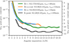 |
Fig. 5 Post-processed contrast of the ERIS gvAPP in the Br-γ, Br-α, Br-α-continuum, and K-peak filters. The contrast curves for the first three filters were calculated after PSF subtraction with optimal PCA/ADI via fake planet injections. The contrast curve for the K-peak filter was calculated with the TRAP algorithm (Samland et al. 2021). The angular separation is shown in units of λ/D in order to compare the results for the different narrow band filters. The central wavelength and effective width of each filter are indicated in the label of each curve. The shaded area represents the uncertainty of the contrast curve. |
3.6 Contrast curves
The resulting contrast curves for each narrow-band filter are shown in Fig. 5. The three Brackett curves approximately match each other up to 6 λ/D, where they reach a contrast of 2.5 × 10⁻⁴ (9 magnitudes). From that point outwards, the two L-band contrast curves flatten due to the increased near-IR background from the atmosphere and warm telescope optics. The Br-γ curve flattens at 10−4 (i.e. 10 mag) around 9–10 λ/D. The K-peak observation reach a contrast deeper by 1.5 mag due to the six times longer integration time. Using the contrast at the largest separation and the corresponding stellar magnitudes in the K and L bands, we computed the sensitivity limits scaled to 1 hour (using the square root of the observing time) in each narrow band. We report the limits for each filter in Table 3.
gvAPP sensitivity limits in narrow-band filters scaled to 1h total on-sky integration time.
Ratio of the coronagraphic PSFs to the leakage term for two nod positions (A and B) on the ERIS detector.
4 Performance analysis
4.1 PSF flux imbalances and sensitivity with the position on the detector
We investigated the relative on-sky throughputs of the central astrometric reference spots in the K-peak data by measuring the ratio of the flux of each spot to the leakage term. To do this, we first extracted the aperture photometry of each spot and the leakage term for each frame in the data. We then divided the photometry of each spot by that of the leakage term, and took the time-averaged mean in each case. These values are shown in Table 4 for two different nod positions, corresponding to opposite sides of the ERIS NIX detector. The ‘left-hand’ and ‘right-hand’ positions of the spots are defined relative to the detector orientation (see the annotations in Fig. 6). The difference between these values is likely due to cross-talk between the readout lines of the sub-arrays in the ERIS detector. The left-hand spot has a brighter background than the leakage term than the right-hand spot at the A nod position, while it is the opposite at the B nod position.
The two coronagraphic PSFs have a brightness asymmetry with one appearing brighter than the other for a given nod position on the ERIS detector. We attribute this difference in flux due to the introduction of circular polarisation within the ERIS optical train, which includes several high incidence reflections that can induce this. In the K-peak data, the brighter coronagraphic PSFs alternated between left-hand and right-hand PSFs, indicating that this effect varies with the position of the star image on the detector (consistent with the explanation above). Average measurements of this asymmetry for the datasets in this paper are given in Table 5. The consequence for observing with the gvAPP in ERIS is that the two nod positions need to be reduced independently with separate flux calibrations for the leakage and coronagraphic PSF.
Flux ratios of the PSFs in the gvAPP.
4.2 Reduced broadband sensitivity
The K-peak observation reaches a sensitivity that is deeper by 2.2 mag compared to the Br-γ curve. If we take the broader filter into account and assume that the sensitivity is proportional to the square root of the transmitted flux through the filters, then the difference in sensitivity is expected to be 0.8 mag between the Br-γ and K-peak filters – assuming that the sky background is the same. Therefore, it seems that the Br-γ observation is not limited by the sky background, but rather by an additional component in the dark hole that could be caused by the brighter star; γ Gru – the star observed for the Br-γ contrast curve – is brighter than HR 8799 by 1.8 mag. The same reasoning can be applied to the Br-α and Br-α-cont observations, for which the broader filter reaches a sensitivity that is deeper by 2.4 mag compared to the narrower filter and where the observed star was fainter by 3 mag.
Detector artefacts can cause this additional noise component in the dark hole and explain the low sensitivity. Figure 6 shows a median-combined frame from the K-peak observation with a colour scale selected to highlight background variations. There is a repeating horizontal pattern on the detector correlated with regions of the PSF with high flux, i.e. the two coronagraphic PSFs and the central leakage term. Both nod positions used to generate Fig. 6 are affected, as there is both a positive and a negative version of this same pattern. The negative pattern originates from the nod position shown in this figure, as this is the one that passes through the centres of the side PSFs and the central leakage term. The positive pattern, which is spatially offset from the negative pattern, aligns with the PSF at the other nod position (not visible in this figure). Both the negative and the positive patterns go through both dark holes, leaving little of the dark hole unaffected. We estimate the effect to be of the order of 10−4 relative to the peak of the APP PSF, with counts of around 4 to 6 compared to 2 × 10⁴ in the core of the APP PSF. These artefacts also appear in our Br-γ observations but not in the Br-α or Br-α-cont observations. We assumed this effect is present in the L band but that the increased thermal background overwhelms this effect. The reason for this pattern is unclear: neither the Br-γ and K-peak observations are saturated and both have detector counts of around 20–30k at the centres of the side PSFs and after background subtraction, which corresponds to approximately 50% of the well depth for the fast readout mode. The periodicity of the pattern suggests electronic cross talk between the readout channels of the ERIS detector caused by the large fluxes of the gvAPP coronagraphic PSFs. For time series observations, this pattern is likely to introduce significant systematics to the obtained photometry. However, it may be possible to largely mitigate these systematics by de-trending using the pixel positions of the star at each nod position as de-correlation parameters, since the pattern is directly correlated with the star’s location on the detector (e.g. Sutlieff et al. 2024, 2025).
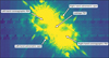 |
Fig. 6 Median combined frame highlighting the impact of the repeating detector noise pattern in the dark holes of the coronagraphic PSFs. The orientation of the image is that of the detector; the left- and right-hand notation is used to describe the positions of the respective PSFs relative to this orientation. |
4.3 Use cases and recommendations
Planetary mass limits have been reached with other gvAPP coronagraphs (e.g. Long et al. 2023) and previous APP coronagraphs of the 180-degree design (e.g. Quanz et al. 2011; Kenworthy et al. 2013; Meshkat et al. 2015a,b). If the orbit of a companion is already well constrained, the user can plan observations to ensure that the companion is positioned centrally in one of the gvAPP dark holes, thereby maximising its signal to noise (e.g. Quanz et al. 2010; Sutlieff et al. 2021). It may therefore be preferable in some cases to use alternative coronagraphs to initially detect a companion before then using the ERIS gvAPP for characterisation.
The ERIS gvAPP design includes features that make it particularly useful for time series studies, such as obtaining measurements of the brightness variability of directly imaged exoplanets and brown dwarf companions. Photometric and spectrophotometric measurements show that many substellar objects exhibit variability as they rotate, thought to originate from inhomogeneous atmospheric features such as patchy clouds, magnetic spots, aurorae, and non-equilibrium chemistry (e.g. Metchev et al. 2015; Vos et al. 2019, 2022; Lew et al. 2020; Biller et al. 2024; Liu et al. 2024; Chen et al. 2025; Tan et al. 2025; Oliveros-Gomez et al. 2026). Measuring the variability of directly imaged companions using ground-based observations is challenging, as a simultaneous photometric reference is required to remove atmospheric and instrumental systematics from the photometry of a companion. Such a photometric reference is unavailable for most coronagraphic observations, but the leakage term or central astrometric spots of gvAPP coronagraphs can be used to correct the photometry of a companion positioned in the dark holes when kept unsaturated. This approach has been previously demonstrated using the central PSF of the LBT dgvAPP and is described in detail in Sutlieff et al. (2023, 2024, 2025).
However, we highlight that while the ERIS gvAPP does provide this built in photometric reference, its throughput and contrast underperformance (5 × 10⁻⁵ on-sky contrast compared to 1 × 10⁻⁵ design contrast) may preclude useful variability studies of known exoplanet companions, as it likely will not be possible to detect them with sufficient signal to noise and cadence (see Table 3). Variability studies with the ERIS gvAPP may therefore only be possible for the brightest companions, such as brown dwarfs, or by compromising on cadence to achieve the necessary signal. Furthermore, we found that there is a slight variance in the brightness of the leakage term relative to the coronagraphic PSFs depending on position on the detector, and the noise patterns shown in Fig. 6 also add position-dependent variance (see Sect. 4.1). Although both of these effects are at a relatively low level and can be mitigated using de-trending techniques (see Sect. 4.2), they will inherently increase the complexity of such observations and may reduce the level of precision that can be achieved.
In order to conduct time series observations with the ERIS gvAPP, it is critical that exposure times are chosen such that the simultaneous astrometric and photometric reference PSFs (i.e. the leakage term) remain unsaturated. We also recommend using the K-peak filter for variability studies using the ERIS gvAPP, as its 6% width is designed to maximise throughput while limiting wavelength smearing to <1λ/D (see Dubber et al. 2022).
For all ERIS gvAPP observations, we strongly recommend using an ABBA nodding pattern to facilitate background subtraction while minimising overheads, with a spacing between the two nod positions such that the gvAPP PSFs do not overlap. The NIX detector has several bad pixel clusters, which dominate large areas of the frame (e.g. see Fig. 2 in Maio et al. 2025), so the two nod positions should therefore be chosen to avoid these regions. This is achieved by setting the alternate nod position to be offset from the default ERIS NIX gvAPP acquisition position by −9.75 arcseconds in the x-direction. It is recommended to use the
window4sub-array, as this frame size remains sufficiently large to fit the gvAPP PSFs at two nod positions while significantly reducing the volume of the data. Further information on the ERIS NIX subarrays and offsetting can be found in the ERIS User Manual3.
The shortest integration time in the smallest available detector window limits the use of normal imaging to stars fainter than mK = 2.6 in the K-peak filter and mL = 0.9 in the Br-α-cont filter. Although brighter stars will saturate, the ERIS gvAPP leakage term can be still be used as a photometric reference of the target if kept unsaturated, and thus it can still be used for photometrically calibrated observations of brighter targets.
5 Conclusions
The gvAPP is built to within the design tolerances specified. The coronagraph throughput, consisting of the (designed) EE throughput, undersizing of the APP telescope pupil, transmission due to the liquid crystal and glue layers, and splitting of target flux between the two coronagraphic PSFs, is consistent with other operating gvAPPs.
The phase pattern successfully pushes the stellar diffraction halo below the wind-driven halo resulting from the partial AO correction of atmospheric turbulence. The on-sky raw contrast is then limited by noise consistent with star light scattered by the optics within the imaging path of ERIS. L-band observations are limited by the large sky background from warm optics in the ERIS optical path and poor transmission due to multiple glue layers in the ERIS gvAPP. In testing, the gvAPP reaches its design specification in transmission with about 90% in the K bands and 60% in the L band. While the gvAPP reaches a considerable raw contrast laboratory performance of 1 × 10⁻⁵, it does not reach the specified 5 × 10⁻⁵: electronic detector pattern noise induced by large amounts of stellar flux causes pixel-scale artefacts within the dark holes of the coronagraphic PSF, limiting the K-band sensitivity.
We recommend the ERIS gvAPP as a tool for studies requiring small IWAs, as gvAPP coronagraphs do not use masks to block target stars. It is particularly suitable for characterising substellar companions with known separations and position angles, which allows them to be positioned in the gvAPP dark holes for observations (e.g. Quanz et al. 2010; Sutlieff et al. 2021; Doelman et al. 2022). Time series observations that use the leakage term as a photometric reference may also be possible for the brightest companions, such as brown dwarfs (e.g. Sutlieff et al. 2024, 2025); however, we note that the contrast performance likely precludes such studies for known high-contrast exoplanets as it will be challenging to achieve the required signal to noise and cadence.
Improvements for ERIS gvAPP data can be made by looking into how to minimise or model the detector electronic noise for removal. Future gvAPP coronagraphs that use the liquid crystal manufacturing technology can increase the throughput if thinner layers of optically active material and optical glues that do not have strong infrared absorption features in them are used. Minimising the number of total glue layers in the final assembled optic of future gvAPP coronagraphs (from ERIS’s four layers down to a minimum of two) will also improve the sensitivity – these lessons have been taken into consideration with the design of the gvAPPs (Absil et al. 2024) for the Extremely Large Telescope (ELT) instruments, including METIS (Brandl et al. 2021). METIS is an ELT instrument with an L- and M-band spectrometer (R∼100 000) that can be used in combination with gvAPPs designed to work with an image slicer and the imaging channels of the instrument. With the ELT’s 39 m diameter, this will allow 2.9–5.3 µm high-resolution spectroscopy and spectral variability measurements to be obtained for directly imaged exoplanets at extremely close separations (e.g. Snellen et al. 2014, 2015; Sutlieff et al. 2023, 2025; Parker et al. 2024; Gandhi et al. 2025).
Data availability
This paper was compiled using the
showyourwork! framework (Luger et al. 2021), which includes all original data files, the computer scripts used to generate the figures, and the associated compilation framework. This is available at https://github.com/mkenworthy/ERIS_gvAPP
Acknowledgements
We thank our referee for a very careful reading of our manuscript and for the improvements this has made. JH acknowledges the financial support from the Swiss National Science Foundation (SNSF) under project grant number 200020_200399. This work has been carried out within the framework of the NCCR PlanetS supported by the Swiss National Science Foundation under grants 51NF40_182901 and 51NF40_205606. BJS and BAB acknowledge funding by the UK Science and Technology Facilities Council (STFC) grant nos. ST/V000594/1 and UKRI1196. JLB acknowledges funding from the European Research Council (ERC) under the European Union’s Horizon 2020 research and innovation program under grant agreement No 805445. AZ acknowledges support from ANID – Millennium Science Initiative Program – centre Code NCN2024_001 and Fondecyt Regular grant number 1250249. This work is based on observations collected at the European Organisation for Astronomical Research in the Southern Hemisphere under ESO programme 112.25QA.001 (PI: Sutlieff). BJS and XC would like to thank Marco Berton, Robert De Rosa, and the support staff at Paranal Observatory for their assistance in obtaining these observations, and Derek McLeod and Britton Smith for their technical advice on cluster computing. This work made use of the University of Edinburgh’s Institute for Astronomy research computing cluster, cuillin, which is partially funded by the UK STFC. We would like to thank Eric Tittley for his work managing and maintaining cuillin. This research has used the SIMBAD database, operated at CDS, Strasbourg, France (Wenger et al. 2000). This work has used data from the European Space Agency (ESA) mission Gaia (https://www.cosmos.esa.int/gaia), processed by the Gaia Data Processing and Analysis Consortium (DPAC, https://www.cosmos.esa.int/web/gaia/dpac/consortium). Funding for the DPAC has been provided by national institutions, in particular the institutions participating in the Gaia Multilateral Agreement. This research has made use of NASA’s Astrophysics Data System. This research made use of SAOImageDS9, a tool for data visualization supported by the Chandra X-ray Science centre (CXC) and the High Energy Astrophysics Science Archive centre (HEASARC) with support from the JWST Mission office at the Space Telescope Science Institute for 3D visualization (Joye & Mandel 2003). To achieve the scientific results presented in this article we made use of the Python programming language4, especially the SciPy (Virtanen et al. 2020), NumPy (Harris et al. 2020), Matplotlib (Hunter 2007), emcee (Foreman-Mackey et al. 2013), astropy (Astropy Collaboration 2013, 2018, 2022), scikit-image (van der Walt et al. 2014), Photutils (Bradley et al. 2022), PynPoint (Amara & Quanz 2012; Stolker et al. 2019), VIP (Gomez Gonzalez et al. 2017; Christiaens et al. 2023), TRAP (Samland et al. 2021), and applefy (Bonse et al. 2023) packages.
References
- Absil, O., Kenworthy, M., Delacroix, C., et al. 2024, SPIE Conf. Ser., 13096, 1309652 [Google Scholar]
- Amara, A., & Quanz, S. P. 2012, MNRAS, 427, 948 [Google Scholar]
- Astropy Collaboration (Robitaille, T. P., et al.) 2013, A&A, 558, A33 [NASA ADS] [CrossRef] [EDP Sciences] [Google Scholar]
- Astropy Collaboration (Price-Whelan, A. M., et al.) 2018, AJ, 156, 123 [Google Scholar]
- Astropy Collaboration (Price-Whelan, A. M., et al.) 2022, ApJ, 935, 167 [NASA ADS] [CrossRef] [Google Scholar]
- Barbato, D., Mesa, D., D’Orazi, V., et al. 2025, A&A, 693, A81 [NASA ADS] [CrossRef] [EDP Sciences] [Google Scholar]
- Berry, M. V. 1984, Proc. Roy. Soc. Lond. A Math. Phys. Eng. Sci., 392, 45 [Google Scholar]
- Biller, B. A., Vos, J. M., Zhou, Y., et al. 2024, MNRAS, 532, 2207 [NASA ADS] [CrossRef] [Google Scholar]
- Boehle, A., Doelman, D., Konrad, B. S., et al. 2021, J. Astron. Telesc. Instrum. Syst., 7, 045001 [NASA ADS] [CrossRef] [Google Scholar]
- Bonse, M. J., Garvin, E. O., Gebhard, T. D., et al. 2023, AJ, 166, 71 [NASA ADS] [CrossRef] [Google Scholar]
- Bos, S. P., Doelman, D. S., Lozi, J., et al. 2019, A&A, 632, A48 [NASA ADS] [CrossRef] [EDP Sciences] [Google Scholar]
- Bradley, L., Sipőcz, B., Robitaille, T., et al. 2022, astropy/photutils: [Google Scholar]
- Brandl, B., Bettonvil, F., van Boekel, R., et al. 2021, The Messenger, 182, 22 [NASA ADS] [Google Scholar]
- Chen, X., Biller, B. A., Tan, X., et al. 2025, MNRAS, 539, 3758 [Google Scholar]
- Christiaens, V., Gonzalez, C., Farkas, R., et al. 2023, J. Open Source Softw., 8, 4774 [NASA ADS] [CrossRef] [Google Scholar]
- Codona, J. L., & Angel, R. 2004, ApJ, 604, L117 [Google Scholar]
- Davies, R., Absil, O., Agapito, G., et al. 2023, A&A, 674, A207 [NASA ADS] [CrossRef] [EDP Sciences] [Google Scholar]
- Doelman, D. S., Snik, F., Por, E. H., et al. 2021, Appl. Opt., 60, D52 [NASA ADS] [CrossRef] [Google Scholar]
- Doelman, D. S., Stone, J. M., Briesemeister, Z. W., et al. 2022, AJ, 163, 217 [NASA ADS] [CrossRef] [Google Scholar]
- Dubber, S., Biller, B., Bonavita, M., et al. 2022, MNRAS, 515, 5629 [Google Scholar]
- Foreman-Mackey, D., Hogg, D. W., Lang, D., & Goodman, J. 2013, PASP, 125, 306 [Google Scholar]
- Gandhi, S., de Regt, S., Snellen, I., et al. 2025, MNRAS, 537, 134 [Google Scholar]
- George, E. M., Gräff, D., Feuchtgruber, H., et al. 2016, Proc. SPIE, 9908, 99080g [Google Scholar]
- Gomez Gonzalez, C. A., Wertz, O., Absil, O., et al. 2017, AJ, 154, 7 [Google Scholar]
- Harris, C. R., Millman, K. J., van der Walt, S. J., et al. 2020, Nature, 585, 357 [NASA ADS] [CrossRef] [Google Scholar]
- Hunter, J. D. 2007, Comput. Sci. Eng., 9, 90 [NASA ADS] [CrossRef] [Google Scholar]
- Joye, W. A., & Mandel, E. 2003, in Astronomical Society of the Pacific Conference Series, 295, Astronomical Data Analysis Software and Systems XII, eds. H. E. Payne, R. I. Jedrzejewski, & R. N. Hook, 489 [NASA ADS] [Google Scholar]
- Kenworthy, M. A., & Haffert, S. Y. 2025, ARA&A, 63, 179 [Google Scholar]
- Kenworthy, M. A., Codona, J. L., Hinz, P. M., et al. 2007, ApJ, 660, 762 [NASA ADS] [CrossRef] [Google Scholar]
- Kenworthy, M., Quanz, S., Meyer, M., et al. 2010, The Messenger, 141, 2 [NASA ADS] [Google Scholar]
- Kenworthy, M. A., Meshkat, T., Quanz, S. P., et al. 2013, ApJ, 764, 7 [Google Scholar]
- Kim, J., Li, Y., Miskiewicz, M. N., et al. 2015, Optica, 2, 958 [Google Scholar]
- Lenzen, R., Hartung, M., Brandner, W., et al. 2003, SPIE Conf. Ser., 4841, 944 [Google Scholar]
- Lew, B. W. P., Apai, D., Zhou, Y., et al. 2020, AJ, 159, 125 [Google Scholar]
- Liu, P., Bohn, A. J., Doelman, D. S., et al. 2023, A&A, 674, A115 [NASA ADS] [CrossRef] [EDP Sciences] [Google Scholar]
- Liu, P., Biller, B. A., Vos, J. M., et al. 2024, MNRAS, 527, 6624 [Google Scholar]
- Long, J. D., Males, J. R., Morzinski, K. M., et al. 2018, SPIE Conf. Ser., 10703, 107032T [NASA ADS] [Google Scholar]
- Long, J. D., Males, J. R., Haffert, S. Y., et al. 2023, AJ, 165, 216 [NASA ADS] [CrossRef] [Google Scholar]
- Luger, R., Bedell, M., Foreman-Mackey, D., et al. 2021, arXiv e-prints [arXiv:2110.06271] [Google Scholar]
- Maio, F., Roccatagliata, V., Fedele, D., et al. 2025, A&A, 698, A52 [NASA ADS] [CrossRef] [EDP Sciences] [Google Scholar]
- Marois, C., Lafrenière, D., Doyon, R., Macintosh, B., & Nadeau, D. 2006, ApJ, 641, 556 [Google Scholar]
- Mesa, D., Gratton, R., D’Orazi, V., et al. 2025, MNRAS, 536, 1455 [Google Scholar]
- Meshkat, T., Kenworthy, M. A., Quanz, S. P., & Amara, A. 2014, ApJ, 780, 17 [Google Scholar]
- Meshkat, T., Bonnefoy, M., Mamajek, E. E., et al. 2015a, MNRAS, 453, 2378 [NASA ADS] [Google Scholar]
- Meshkat, T., Kenworthy, M. A., Reggiani, M., et al. 2015b, MNRAS, 453, 2533 [NASA ADS] [Google Scholar]
- Metchev, S. A., Heinze, A., Apai, D., et al. 2015, ApJ, 799, 154 [NASA ADS] [CrossRef] [Google Scholar]
- Miller, K., Males, J. R., Guyon, O., et al. 2019, J. Astron. Telesc. Instrum. Syst., 5, 049004 [Google Scholar]
- Miller, K. L., Bos, S. P., Lozi, J., et al. 2021, A&A, 646, A145 [NASA ADS] [CrossRef] [EDP Sciences] [Google Scholar]
- Oliveros-Gomez, N., Manjavacas, E., Karalidi, T., et al. 2026, ApJ, 997, 136 [Google Scholar]
- Orban de Xivry, G., Absil, O., De Rosa, R. J., et al. 2024, SPIE Conf. Ser., 13097, 1309715 [Google Scholar]
- Otten, G. P. P. L., Snik, F., Kenworthy, M. A., Miskiewicz, M. N., & Escuti, M. J. 2014, Opt. Express, 22, 30287 [CrossRef] [Google Scholar]
- Otten, G. P., Snik, F., Kenworthy, M. A., et al. 2017, ApJ, 834, 175 [NASA ADS] [CrossRef] [Google Scholar]
- Pancharatnam, S. 1956, Proc. Indian Acad. Sci. A, 44, 247 [Google Scholar]
- Parker, L. T., Birkby, J. L., Landman, R., et al. 2024, MNRAS, 531, 2356 [Google Scholar]
- Pearson, D., Taylor, W., Davies, R., et al. 2016, SPIE Conf. Ser., 9908, 99083F [NASA ADS] [Google Scholar]
- Por, E. H., Haffert, S. Y., Radhakrishnan, V. M., et al. 2018, in Proc. SPIE, 10703, Adaptive Optics Systems VI [Google Scholar]
- Quanz, S. P., Meyer, M. R., Kenworthy, M. A., et al. 2010, ApJ, 722, L49 [Google Scholar]
- Quanz, S. P., Kenworthy, M. A., Meyer, M. R., Girard, J. H. V., & Kasper, M. 2011, ApJ, 736, L32 [Google Scholar]
- Quanz, S. P., Amara, A., Meyer, M. R., et al. 2013, ApJ, 766, L1 [Google Scholar]
- Rousset, G., Lacombe, F., Puget, P., et al. 2003, SPIE Conf. Ser., 4839, 140 [Google Scholar]
- Ruane, G., Riggs, A., Mazoyer, J., et al. 2018, SPIE Conf. Ser., 10698, 106982S [NASA ADS] [Google Scholar]
- Samland, M., Bouwman, J., Hogg, D. W., et al. 2021, A&A, 646, A24 [NASA ADS] [CrossRef] [EDP Sciences] [Google Scholar]
- Snellen, I. A. G., Brandl, B. R., de Kok, R. J., et al. 2014, Nature, 509, 63 [Google Scholar]
- Snellen, I., de Kok, R., Birkby, J. L., et al. 2015, A&A, 576, A59 [NASA ADS] [CrossRef] [EDP Sciences] [Google Scholar]
- Snik, F., Otten, G., Kenworthy, M., et al. 2012, SPIE Conf. Ser., 8450 [Google Scholar]
- Stolker, T., Bonse, M. J., Quanz, S. P., et al. 2019, A&A, 621, A59 [NASA ADS] [CrossRef] [EDP Sciences] [Google Scholar]
- Sutlieff, B. J., Bohn, A. J., Birkby, J. L., et al. 2021, MNRAS, 506, 3224 [NASA ADS] [CrossRef] [Google Scholar]
- Sutlieff, B. J., Birkby, J. L., Stone, J. M., et al. 2023, MNRAS, 520, 4235 [NASA ADS] [CrossRef] [Google Scholar]
- Sutlieff, B. J., Birkby, J. L., Stone, J. M., et al. 2024, MNRAS, 531, 2168 [Google Scholar]
- Sutlieff, B. J., Doelman, D. S., Birkby, J. L., et al. 2025, MNRAS, 544, 3191 [Google Scholar]
- Tan, X., Zhang, X., Marley, M. S., et al. 2025, Sci. Adv., 11, 22.3324 [Google Scholar]
- van der Walt, S., Schönberger, J. L., Nunez-Iglesias, J., et al. 2014, PeerJ, 2, e453 [Google Scholar]
- Virtanen, P., Gommers, R., Oliphant, T. E., et al. 2020, Nat. Methods, 17, 261 [Google Scholar]
- Vos, J. M., Biller, B. A., Bonavita, M., et al. 2019, MNRAS, 483, 480 [NASA ADS] [Google Scholar]
- Vos, J. M., Faherty, J. K., Gagné, J., et al. 2022, ApJ, 924, 68 [NASA ADS] [CrossRef] [Google Scholar]
- Wagner, K., Stone, J., Dong, R., et al. 2020, AJ, 159, 252 [NASA ADS] [CrossRef] [Google Scholar]
- Wenger, M., Ochsenbein, F., Egret, D., et al. 2000, A&AS, 143, 9 [NASA ADS] [Google Scholar]
See the ERIS instrument description for filter definitions: https://www.eso.org/sci/facilities/paranal/instruments/eris/inst.html
ERIS User Manual: https://www.eso.org/sci/facilities/paranal/instruments/eris/doc.html.
All Tables
Design parameters for the ERIS gvAPP including the inner working angle (IWA) and outer working angle (OWA).
gvAPP sensitivity limits in narrow-band filters scaled to 1h total on-sky integration time.
Ratio of the coronagraphic PSFs to the leakage term for two nod positions (A and B) on the ERIS detector.
All Figures
|
Fig. 1 ERIS gvAPP phase pattern design and simulated PSF. Left: phase within the defined gvAPP pupil. Right: resultant three PSFs of the gvAPP. We show the two coronagraphic PSFs and the central leakage term. Three astrometric reference spots can be seen. The scale is logarithmic in normalised intensity. |
| In the text | |
|
Fig. 2 Optical transmission of the gvAPP measured in the laboratory (black curve) and the on-sky background transmission in the Br-α filter (orange point). Additional measurements with the ERIS internal calibration unit are shown by the blue points. The blue regions trace all filters available for observations with the gvAPP in ERIS. Note that for on-sky throughput, this transmission curve should be multiplied by 0.23 to account for the EE and division of the flux between coronagraphic PSFs (see Sect. 3.2). |
| In the text | |
|
Fig. 3 Geometry of combining the two coronagraphic PSFs to form the coverage around the target star. The hatched area is masked out during subsequent image combination and processing. The semi-circular dashed lines are a visual aid only; the area at wider separations beyond these circles is not masked in the combined image. |
| In the text | |
|
Fig. 4 Raw contrast of the gvAPP in the Br-α-continuum filter. Left: raw flux contrast evaluated in λ/D-sized apertures placed in the dark hole over an aperture placed on the PSF centre in the left lobe of a deep integration on HR 8799 at 3.96 µm. The orange line traces the median contrast evaluated in a ±10◦ region perpendicular to the main axis of the gvAPP PSF. The orange markers indicate the IWA and OWA provided in Table 1. The blue curve displays the raw contrast measured on the gvAPP element under laboratory conditions at 2 µm by Boehle et al. (2021) – the values from 10 to 12.5 λ/D are below the sensitivity of the test bench. The rise seen at 13.5 λ/D in the laboratory data is due to limitations from internal reflections in the test bench not present in ERIS. Right: focal plane image of the left lobe of the gvAPP on which the raw contrast was evaluated. The shaded orange wedge is the ±10◦ region in which the orange contrast curve was measured. |
| In the text | |
|
Fig. 5 Post-processed contrast of the ERIS gvAPP in the Br-γ, Br-α, Br-α-continuum, and K-peak filters. The contrast curves for the first three filters were calculated after PSF subtraction with optimal PCA/ADI via fake planet injections. The contrast curve for the K-peak filter was calculated with the TRAP algorithm (Samland et al. 2021). The angular separation is shown in units of λ/D in order to compare the results for the different narrow band filters. The central wavelength and effective width of each filter are indicated in the label of each curve. The shaded area represents the uncertainty of the contrast curve. |
| In the text | |
|
Fig. 6 Median combined frame highlighting the impact of the repeating detector noise pattern in the dark holes of the coronagraphic PSFs. The orientation of the image is that of the detector; the left- and right-hand notation is used to describe the positions of the respective PSFs relative to this orientation. |
| In the text | |
Current usage metrics show cumulative count of Article Views (full-text article views including HTML views, PDF and ePub downloads, according to the available data) and Abstracts Views on Vision4Press platform.
Data correspond to usage on the plateform after 2015. The current usage metrics is available 48-96 hours after online publication and is updated daily on week days.
Initial download of the metrics may take a while.