| Issue |
A&A
Volume 708, April 2026
|
|
|---|---|---|
| Article Number | A158 | |
| Number of page(s) | 10 | |
| Section | Astrophysical processes | |
| DOI | https://doi.org/10.1051/0004-6361/202558541 | |
| Published online | 03 April 2026 | |
PSR J0024–7204ai: A massive eccentric binary system in the globular cluster 47 Tucanae
1
Max-Planck-Institut für Radioastronomie, Auf dem Hügel 69, D-53121 Bonn, Germany
2
Rheinische Friedrich-Wilhelms-Universität Bonn, Regina-Pacis-Weg 3, D-53113 Bonn, Germany
3
Fakultät für Physik, Universität Bielefeld, D-33615 Bielefeld, Germany
4
Dipartimento di Fisica e Astronomia, Università degli Studi di Bologna, Via Gobetti 93/2, I-40129 Bologna, Italy
5
INAF, Osservatorio di Astrofisica e Scienza dello Spazio di Bologna, Via Gobetti 93/3, I-40129 Bologna, Italy
6
INAF – Osservatorio Astronomico di Cagliari, Via della Scienza 5, I-09047 Selargius (CA), Italy
7
South African Radio Astronomy Observatory, 2 Fir Street, Black River Park, Observatory 7925, South Africa
8
Max Planck Institute for Gravitational Physics (Albert Einstein Institute), D-30167 Hannover, Germany
9
Leibniz Universität Hannover, D-30167 Hannover, Germany
10
National Astronomical Observatories, Chinese Academy of Sciences, A20 Datun Road, Chaoyang District, Beijing 100101, PR China
11
Centre for Astrophysics and Supercomputing, Swinburne University of Technology, P.O. Box 218 Hawthorn, VIC 3122, Australia
★ Corresponding authors: This email address is being protected from spambots. You need JavaScript enabled to view it.
, This email address is being protected from spambots. You need JavaScript enabled to view it.
Received:
12
December
2025
Accepted:
13
February
2026
Abstract
In this paper we present PSR J0024−7204ai, a 13.026-ms binary pulsar recently discovered in the globular cluster 47 Tucanae by the MeerKAT radio telescope. This is the slowest-spinning pulsar known in this globular cluster. It has a ∼1.67-day orbit with an eccentricity of e ≈ 0.18. Although it is not yet possible to derive an unambiguous phase-connected timing solution, by combining detections obtained from MeerKAT and archival Parkes data, we were able to measure the rate of advance of periastron to a high significance: ω˙ = 0.1601 ± 0.0046 deg yr−1. This value implies a total system mass of 2.41 ± 0.11 M⊙ (68.3% C.L.), which, when combined with the binary mass function, gives a maximum pulsar mass of ∼1.7 M⊙ and a minimum companion mass of ∼0.7 M⊙. Apart from being the slowest pulsar in 47 Tucanae, its orbit is by far the most eccentric, and its companion is the most massive among all known binary pulsars in this globular cluster. It is possible that the system is an old millisecond pulsar–carbon-oxygen white dwarf binary whose orbit was perturbed by stellar dynamical interactions in the cluster core. Further follow-up observations of this system will be essential to obtaining a more detailed characterisation of this system and its evolution.
Key words: binaries: general / stars: neutron / pulsars: individual: 47 Tucanae
© The Authors 2026
 Open Access article, published by EDP Sciences, under the terms of the Creative Commons Attribution License (https://creativecommons.org/licenses/by/4.0), which permits unrestricted use, distribution, and reproduction in any medium, provided the original work is properly cited.
This article is published in open access under the Subscribe to Open model.
Open access funding provided by Max Planck Society.
1. Introduction
Globular clusters (GCs) are gravitationally self-bound Galactic sub-systems consisting of 104 to 106 stars. They are also among the oldest stellar systems in the Galaxy, with their ages ranging from 10 to 13 billion years–comparable to the age of the Universe. In their cores, the stellar density can be as high as 105 to 106 M⊙ pc−3 (Baumgardt & Hilker 2018), which are a few orders of magnitude higher than what is typically seen in the Galactic field. These extremely dense environments enhance two- or three-body stellar dynamical interactions and the formation of the binary stellar systems (Hills 1975; Verbunt & Hut 1987; Sigurdsson & Phinney 1995).
In such exchange encounters, old and ‘dead’ neutron stars (NSs; i.e. NSs that have crossed the death line and whose emission is no longer detectable) can become members of binary systems with low-mass main sequence stellar companions. As the companion star evolves according to the standard theory of stellar evolution and fills its Roche lobe, the mass and angular momentum is transferred to the NS. This accretion of matter onto the NS surface makes the pair visible in X-ray wavelengths as a low-mass X-ray binary (LMXB). The LMXBs per unit of stellar mass are orders of magnitude more numerous in GCs than in the Galactic disc (Clark 1975).
Due to the relatively slower evolution of the low-mass companion, the LMXB phase is long-lived and can spin up the NS to rotation periods of just a few milliseconds, giving birth to a radio millisecond pulsar (MSP). This process is known as ‘pulsar recycling’ (Radhakrishnan & Srinivasan 1982; Alpar et al. 1982; Bhattacharya & van den Heuvel 1991; Papitto et al. 2013, for a review see Tauris & van den Heuvel 2023). The large rate of formation of LMXBs in GCs is the reason why a wealth of MSPs (P < 10 ms) are seen in these environments1. Such MSPs are formed with very low, near-zero eccentric orbits due to the tidal circularisation.
If the companion is a main-sequence star significantly more massive than 1 M⊙, the systems become intermediate-mass and high-mass X-ray binaries, respectively. These have relatively short-lived mass transfer phases since the companion evolves faster. The pulsar is spun-up to spin periods between 10 to 200 ms, resulting in a mild recycling (Tauris & van den Heuvel 2006). The companion stars in these systems are relatively massive CO white dwarfs (WDs) or ONeMg WDs, in which case the orbits have very low eccentricities, e ≲ 10−3 (Tauris et al. 2000, 2011, 2012), or in some cases they are NSs (Tauris et al. 2017) with e ∼ 0.1 or larger. However, it is important to point out that such massive main-sequence companions were only available in the earlier stages of the evolution of the GCs.
The binary MSPs in GCs are particularly interesting because of stellar perturbations, which can make them acquire significant eccentricities even if they are born circular. In some cases, these stellar encounters lead to exchange interactions, where a low-mass companion to an already recycled pulsar is exchanged by a more massive star, like M15C (Prince et al. 1991), NGC 1851A, D and E (Freire et al. 2004; Ridolfi et al. 2022; Barr et al. 2024), NGC 6624G (Ridolfi et al. 2021), M30B (Balakrishnan et al. 2023), and NGC 6544B (Lynch et al. 2012). These systems are therefore ‘secondary exchange encounters’. Their large eccentricities and companion masses imply that with several years of timing data, relativistic post-Keplerian (PK) parameters such as the rate of advance of periastron ( ), the Einstein delay (γE), or the two parameters characterising the Shapiro delay (Shapiro 1964) become measurable, thus allowing a determination of the masses (Lynch et al. 2012; Dutta et al. 2025) and in some cases (e.g. that of PSR B2127+11C) tests of general relativity (Jacoby et al. 2006). However, this type of binaries are only found in GCs where the rate of stellar interactions per binary (γ) is large (Verbunt & Freire 2014).
The GC NGC 104, or alternatively 47 Tucanae (47 Tuc here on), is located in the southern hemisphere at equatorial sky coordinates α = 00h 24m 05.67s, δ = −72° 04′ 52.6″, or Galactic coordinates l = 305.89°, b = −44.89°, at a distance of 4.69 kpc from the Sun (Woodley et al. 2012). Its age estimates vary from 10.4 to 13.4 Gyr (Gratton et al. 2003; Brogaard et al. 2017; Thompson et al. 2020). Several past discoveries and timing studies of the pulsars in 47 Tuc (Manchester et al. 1990, 1991; Robinson et al. 1995; Camilo et al. 2000; Ridolfi et al. 2016; Freire et al. 2017) enabled studies of cluster dynamics, mass segregation, and gravitational potential as well as the detection of ionised gas in the cluster (Freire et al. 2001a; Abbate et al. 2018, 2023). The precise positions allowed X-ray detections of all pulsars with known timing solutions (Grindlay et al. 2002; Bogdanov et al. 2005, 2006; Bhattacharya et al. 2017; Hebbar et al. 2021). Of the 13 binaries with precise positions, five white dwarf companions (Edmonds et al. 2001; Rivera-Sandoval et al. 2015; Cadelano et al. 2015) and one redback (Edmonds et al. 2002) companion were detected and characterised in archival Hubble Space Telescope images.
This scientific payoff motivated MeerKAT observations of 47 Tuc, which began under the TRAPUM2 project (Stappers & Kramer 2016) in May 2020. The main aim has been to discover new pulsars, but the observations are also used to measure the masses of some of the previously known pulsars. At the time of writing, the project has discovered 17 pulsars in the cluster (Ridolfi et al. 2021; Chen et al., in prep.). Of these new discoveries, at least 14 are binary pulsars, and the total percentage of binaries is now 69% (i.e. 29/42).
Unlike the binary systems in some other GCs (e.g. Terzan 5; Padmanabh et al. 2024), all the binaries in 47 Tuc have low (< 0.1) orbital eccentricities and companion masses. This is expected for GCs like 47 Tuc that has a relatively low value of γ; i.e. once a LMXB forms, it evolves into a circular MSP–low-mass companion system without much risk of being perturbed, at least for the systems with smaller orbital periods, where the cross section for interactions is smaller.
One of the newly discovered pulsars, PSR J0024−7204ai (henceforth referred to as 47 Tuc ai) is the exception among the binaries in 47 Tuc, and it is the topic of this work. As described below, its spin period of 13.026 ms makes it the first mildly recycled pulsar in 47 Tuc. Its eccentric binary orbit (e ≃ 0.18) and large companion mass also make it stand out from the remaining pulsar population. The structure of the paper is as follows: In Sect. 2, we give an overview of the dataset used for this work. Sect. 3 focuses on the determination of the orbit, localisation, and basic emission characteristics and an early timing analysis. In Sect. 4 we discuss the nature and origin of this binary system. In Sect. 5, we summarise our results and discuss some near-future prospects.
2. Observations
2.1. MeerKAT observations
Between 2019 March and 2024 January, 47 Tuc was observed with the South African MeerKAT radio telescope array on 41 occasions. The observations were made as part of the TRAPUM and MeerTime3 (Bailes et al. 2020) large survey projects and had a number of different scientific aims. Therefore the set-ups and observing parameters of the whole dataset are highly heterogeneous. The observations carried out under MeerTime, which had pulsar timing as the main scientific driver, made use of the Pulsar Timing User Supplied Equipment (PTUSE) as the primary backend. PTUSE is capable of recording up to four tied-array beams on the sky, and it records the data as coherently de-dispersed search-mode PSRFITS files with full-Stokes information. Given the small number of beams that could be synthesised, the PTUSE beams were produced correlating only the central 44 1-km-core antennas of the MeerKAT array to have a larger field of view at the cost of a roughly 30% reduction in raw sensitivity. Observations carried out under TRAPUM, whose main goal was the discovery of several new pulsars, made use of the Filterbanking Beamformer User Supplied Equipment (FBFUSE) and the Accelerated Pulsar Search User Supplied Equipment (APSUSE) as the primary backend. These enabled the synthesis of up to 288 tied-array beams on the sky, which in turn allowed for coverage of a much larger sky area around the cluster centre compared to PTUSE, even correlating the raw signals coming from all the available (up to 64) MeerKAT antennas, hence retaining maximum sensitivity. In this case, each beam could be recorded as a search-mode total-intensity ‘filterbank’ file without coherent de-dispersion. However, since the DM of 47 Tuc is well known, the TRAPUM beams were typically recorded with 4096 frequency channels and later incoherently de-dispersed at a DM of 24.4 pc cm−3 and summed in groups of 16 to reduce the number of channels to 256. In the vast majority of the observations, both PTUSE and FBFUSE+APSUSE were used in parallel. All the observations were made with either the UHF band (544−1088 MHz) or the L band (856−1712 MHz) receivers. The details of all the observations used in this work are reported in Table A.1.
2.2. Parkes archival data
Given the highly negative −72 deg declination of the GC 47 Tuc, it could only be observed by the radio telescopes in the southern hemisphere. Before the MeerKAT radio telescope became operational, it was possible to observe this GC only with the Parkes radio telescope in Australia. With the latter, observations of 47 Tuc were regularly carried out from 1997 to 2013 with the Multibeam receiver (Staveley-Smith et al. 1996) for a total of approximately 1770 observing hours, split across 414 observation epochs (i.e. days) and 519 total pointings4. For a detailed description of the dataset and its previous uses, refer to Ridolfi et al. (2016).
From the year 2019 onwards, the Parkes radio telescope was equipped with the Ultra-Wide bandwidth Low receiver (UWL) (Hobbs et al. 2020), capable of observing in the frequency range 704−4032 MHz. A few observations of 47 Tuc were made with this receiver in the context of different projects (see Table A.2) and are available on the CSIRO Data Access Portal. These observations were also processed in the context of this work.
3. Preliminary characterisation
3.1. Discovery and orbital parameters
Pulsar 47 Tuc ai was first detected in the MeerKAT observation ‘11L’ as a 13.026-ms candidate with a barycentric line of sight acceleration of 4.02 m s−2 and a DM = 24.47 pc cm−3 (we refer to Chen et al., in prep. for more details about the search). The large acceleration clearly pointed towards its binary nature. The candidate was soon confirmed to be a real pulsar based upon its detections in neighbouring beams of the 11L observation and by a few additional detections in other observations. In the first TRAPUM observing campaign on 47 Tuc, the pulsar was blindly detected in seven observations, two of which were made in the L band and five others in the UHF band. Plotting the measured spin periods versus the line-of-sight accelerations (Fig. 1) in a period-acceleration diagram (Freire et al. 2001b, corrected as per the erratum Freire et al. 2009) revealed a mild orbital eccentricity and allowed for a first estimate of the orbital parameters: The pulsar is in an orbit with an orbital period of Pb ≃ 1.65 days and a projected semi-major axis of xp ≃ 5.35 s, an eccentricity of e ≃ 0.18, and a periastron longitude of ω ≃ 227°.
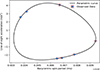 |
Fig. 1. Period-acceleration diagram for 47 Tuc ai. The data points are the barycentric spin periods and line-of-sight accelerations as measured on seven different epochs where the pulsar was blindly detected. The best-fit parametric curve (solid black line), from Eqs. (3) and (4) from Freire et al. (2001c), largely deviates from a simple ellipse, implying a mild orbital eccentricity (e ≈ 0.18). |
After building a basic ephemeris with these parameters, we used the spider_twister5 software to find the precise times of passage at periastron (T0) closest to each detection epoch. These were used to apply the periodogram method (see e.g. Ridolfi et al. 2016), which allows for a refinement of Pb by finding a value of Pb that fits an integer number of times between any two T0 values. Finally, we used the fitorb.py code from the PRESTO6 pulsar searching software (Ransom 2001) to directly fit the observed spin period of the pulsar as a function of time, which significantly improved the precision of the orbital parameters. The refined parameters were used to update the pulsar ephemeris, which was in turn used to re-fold the whole Parkes and MeerKAT datasets. In doing so, we allowed for a full-orbit search in the value of T0 with spider_twister to account for a possible wrong orbital phase prediction due to a possibly still inaccurate Pb. This led to the detection of 47 Tuc ai in a few additional MeerKAT observations, where the pulsar was not detected blindly, as well as in three different Parkes observations dating back to the year 2000. These are listed in Table 1. The three Parkes detections turned out to be very important for the precise measurement of the periastron advance (see Sect. 3.4).
Observations of 47 Tuc made by the Parkes radio telescope with the Multibeam receiver in which pulsar 47 Tuc ai was detected.
3.2. SEEKAT localisation
The MeerKAT observations performed under the TRAPUM project recorded up to 288 synthesised coherent beams in a dense tiling spanning a few arcminutes around the centre of 47 Tuc. This unique capability of the TRAPUM recording system enables determination of the sky position of newly discovered pulsars to arcsecond precision using just a single observation. The individual coherent beams have an average full-width at half maximum (FWHM) of ≈16 arcsec on the sky for the UHF band (central frequency of 816 MHz). The detection of any pulsar in a given beam indicates that the true position of the pulsar is within the beam FWHM or quite close to the beam bore-sight. Given that a pulsar has detections in multiple surrounding beams, this information can be exploited to find the true position with higher accuracy. We used the SEEKAT software (Bezuidenhout et al. 2023), which takes the positions and point spread function of multiple coherent beams and the detection S/N values in those beams to run a maximum likelihood analysis of the position of the pulsar. The SEEKAT maximum likelihood position for 47 Tuc ai was found to be at right ascension  and declination
  , where the uncertainties are at a 1σ confidence level. Fig. 2 shows the localised position of the pulsar with respect to the cluster centre.
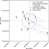 |
Fig. 2. SEEKAT localisation of 47 Tuc ai, with the 1σ uncertainty on the localised position shown as a magenta coloured ellipse. The grey ellipses are beams from the observation 26U1 in which the pulsar was detected at the highest S/N, and they were used for localising the pulsar as discussed in Sect. 3.2. The centre of the GC 47 Tuc (central cross), the core radius (blue circle), and the positions of some of the known pulsars in 47 Tuc are shown for reference. The image covers an area of 1 arcmin × 1 arcmin around the centre of the GC 00h 24m 05.67s, −72° 04′ 52.6″ (Woodley et al. 2012). |
3.3. Pulse profile evolution with frequency
A strong variation of the integrated pulse profile with observing frequency is observed for 47 Tuc ai. This phenomenon is documented in Figs. 3 and 4, where we show the brightest detection of the pulsar as seen in different sub-bands of the MeerKAT L, MeerKAT UHF, and Parkes 1300-MHz bands. In Fig. 3, it can be clearly seen that the relative height between the two components changes as a function of frequency, with the second component becoming brighter with increasing frequency.
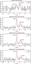 |
Fig. 3. Evolution of pulse profile of PSR 47 Tuc ai with observing frequency. The profile components are marked with Comp1 and Comp2. Each sub-plot shows the pulse profile at different observing frequencies in black and 2-component Gaussian fits to the profile in dotted red lines. The profiles have been normalised in the amplitude. The results obtained from fit – relative amplitudes, widths and separation between the components are reported in Table 2. |
We quantified this effect by fitting each of the two components with a Gaussian and by measuring their amplitudes, widths, and relative separation in each sub-band. The results of the fitting are summarised in Table 2 and shown graphically in Fig. 4. We do not discuss the implications of this effect, as the topic is beyond the scope of this paper.
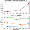 |
Fig. 4. Variation of relative amplitudes, widths and separation between two components of the pulse profile with respect to observing frequency. The fitted profiles at different frequency are shown in Fig. 3 and fitting statistics are listed in Table 2. It can be seen from the upper sub-plot that the relative amplitude of first component increases as a function of observing frequency. |
Profile evolution of pulsar 47 Tuc ai.
3.4. Timing
After the determination and refinement of the orbital parameters, we proceeded with the timing analysis for 47 Tuc ai, attempting to derive the phase-connected timing solution (i.e. an ephemeris that can unambiguously count every rotation of the pulsar over the time span of the data). We used the software dspsr7 (van Straten & Bailes 2011) to fold the search-mode data of all the observations in which the pulsar was detected. We did this using an ephemeris containing the rotational and orbital parameters, obtained as described in the previous section.
The folded archive files were then cleaned from radio frequency interference by using the pazi routine of the PSRCHIVE8 software (Hotan et al. 2004), which was re-called from alex_clean_archives9, a Python-based wrapper of the program that helps automate the cleaning of large datasets. We then created a standard profile using the detection of 47 Tuc ai of the MeerKAT UHF observation 26U1, as the pulsar was detected in it with the highest signal-to-noise ratio. The integrated pulse profile of that detection was fitted with von Mises functions using paas from PSRCHIVE to obtain a noise-free template.
The topocentric pulse times of arrival (ToAs) were then extracted by cross-correlating the template against an appropriate set of sub-integrations and possible sub-bands from each folded archive. This was done using alex_toasel10, another Python-based wrapper that calls the PSRCHIVE’s pat routine.
The ToAs were fitted for the timing model parameters using the TEMPO11 pulsar timing software (Nice et al. 2015). Initially, we kept ‘JUMP’ statements between consecutive groups of locally phase-connected ToAs from the individual observations. These JUMPs allow TEMPO to fit for arbitrary time offsets between the groups of ToAs. MeerKAT observations 25U to 28U (see Table A.1) were part of a second observing campaign made over three days. These had frequent bright detections of 47 Tuc ai, which were easily manually phase connected. This means that we could start determining the number of rotations between the observations without any ambiguities. We attempted to do so with DRACULA12, a software developed by Freire & Ridolfi (2018) that automatically determines the rotation counts of pulsars starting from the given input ephemeris. Since there were only 59 ToAs spanning the timing baseline of nearly 25 years, the dataset was sparse and contained irregular detections and large gaps of tens of years with no ToAs. Due to this limitation of the dataset, we could not find an unambiguous phase-connected timing solution. The results presented here have ToAs from observations 25U to 28U manually connected, and the rest are jumped. The resulting parameters are presented in Table 3, and the post-fit timing residuals are plotted in Fig. 5.
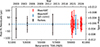 |
Fig. 5. Post-fit timing residuals of 47 Tuc ai as per the timing solution in Table 3. The groups of ToAs are marked in different colours as follows: red – MeerKAT (jumped); blue – MeerKAT phase-connected; black – Parkes Multibeam. |
Parameters of 47 Tuc ai from the partially connected timing solution.
Any MeerKAT data taken with the APSUSE system in the UHF band before 21 January 2022 and in the APSUSE L band taken before 28 January 2021 may occasionally suffer positive time offsets due to heap losses in the data recoding. These time offsets cannot be trivially determined. Hence, the ToAs generated from the data in observations 10L, 11L, 12U, 15L, 17L, 18U, 20U, and 21U could not be confidently included when attempting the phase connection, and they were necessarily jumped. In the future, while attempting the phase connection, it will be important to compensate for this issue.
3.5. Measurement of the mass function and 
Once the Keplerian parameters are known, the binary mass function can be calculated as follows:
 (1)
(1)
where T⊙ = 𝒢ℳ⊙N/c3 = 4.925490947… μs is an exact quantity, the solar mass parameter (Prša et al. 2016) in time units, and Mp, Mc are the masses of pulsar and the companion, respectively. In any equation with T⊙, the masses are dimensionless. We added the unit M⊙ to make it clear that the masses are in multiples of the solar mass parameter.
Despite the lack of a phase-connected timing solution, the combination of the large eccentricity and large semi-major axis of the system allowed for a highly significant estimate of the rate of advance of the periastron,  deg yr−1. This precise measurement greatly benefited from the addition of Parkes ToAs from the year 2000, 2004, and 2013, making a total 25-year timing baseline.
Assuming  is fully relativistic effect, then in general relativity it is given by (Robertson 1938; Taylor & Weisberg 1982)
 (2)
(2)
where Mtot is the total mass of the system (pulsar plus companion). The measured value of  implies Mtot = 2.41 ± 0.11 M⊙. In combination with the mass function, this results in constraints on the pulsar and companion masses (Fig. 6): The maximum pulsar mass (Mp, max) is 1.7 M⊙, and the minimum companion mass (Mc, min) is 0.7 M⊙. For Mp = 0, the minimum sin i is 0.284, which implies i ≥ 16.5°.
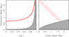 |
Fig. 6. Mass-mass diagram of 47 Tuc ai. The plot on the left shows Mc as a function of cos i, while i is the inclination of the system. The plot on the right shows Mc as a function of Mp. The grey region in the left plot is excluded, as it implies negative Mp. For the plot on the right, the grey region is excluded by the mass function and the constraint that sin i ≤ 1. The red lines in both the plots show nominal values and the total mass derived from |

4. Nature and origin of the system
The previously known pulsar population in 47 Tuc closely resembles the population of fast-spinning MSPs in the Galactic disc (Ridolfi et al. 2016; Freire et al. 2017). All of the pulsars have a low-mass companion with an orbit that is circular or with a low eccentricity. However, in the case of 47 Tuc H, and to a lesser extent 47 Tuc E, the eccentricity is significantly raised by interactions with other stars.
The pulsar 47 Tuc ai qualifies simultaneously for three records within the pulsar population currently known in 47 Tuc: (i) it is the slowest spinning and only one mildly recycled pulsar; (ii) its orbital eccentricity is highest among all the binary pulsars; (iii) its companion is most massive among all the binary pulsar companions. It is clearly different from other MSP–Helium WD systems in the cluster since for this orbital period, the mass of a He-WD companion should be about 0.2 M⊙ (Tauris & Savonije 1999).
The large system mass (Mtot = 2.41 ± 0.11 M⊙), companion mass (Mc > 0.7 M⊙), and the orbital eccentricity are close to what one finds among double NS (DNS; for a review see Tauris et al. 2017) systems, as can be seen in Fig. 7, where 47 Tuc ai appears with a magenta colour near a horizontal clump where the Galactic DNSs are located. Recently, one such system was found in a GC, M71D (Lian et al. 2025), which is thought to have formed from the original population of massive stars in that GC. Despite the fact that the total mass is still consistent (within 1σ) with the lightest DNSs in the Galaxy (Martinez et al. 2017; Meng et al. 2025), the nominal value indicates a lower total mass. Furthermore, the spin period is shorter than the 17 ms observed for PSR J1946+2052, the fastest-spinning pulsar in a DNS known (Stovall et al. 2018; Meng et al. 2025).
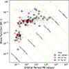 |
Fig. 7. Mass function plotted against the orbital period for all the binary pulsars from the ATNF pulsar catalogue (https://www.atnf.csiro.au/research/pulsar/psrcat/) (Manchester et al. 2005). The binary pulsars in the Galactic field are shown with filled grey dots, while the pulsars in GC are circles. Pulsars in GC 47 Tuc are in red, and those in other GCs are shown with black circles. The inclined dotted yellow lines represent the constant projected semi-major axis of the binary orbit, which is smallest at the lower-left side: x = 1 lt-millisecond. From the bottom left to the top right, the successive dotted yellow lines are an order of magnitude greater than the previous one. The magenta coloured star symbol represents the 47 Tuc ai system. |
Another possibility is that the system is an exchange encounter. Several exchange encounters have been found in GCs that superficially resemble DNSs, including PSR B2127+11C in the GC M15 (P = 30.5 ms, Pb = 8 h, e = 0.68). When the characteristic age of this pulsar was measured, Prince et al. (1991) suggested that the system likely had a low-mass companion at an early stage, which partially recycled it, and that at a later stage the pulsar acquired its current more massive companion in an exchange interaction. This massive degenerate companion can therefore either be a massive WD or a NS. Thus, dynamically, PSR B2127+11C is a secondary exchange encounter. However, this origin for 47 Tuc ai is also unlikely because systems going through an exchange encounter typically retain higher eccentricities (for systems where it is clearer that this is the origin, 0.38 < e < 0.90); the orbital eccentricity of PSR B2127+11C is typical of such systems. Furthermore, secondary exchange encounters are most likely to form in GCs with a high γ, for 47 Tuc this number is much lower than those of M15, NGC 6544 or NGC 1851, where undoubted secondary exchange products have been found.
Therefore, the most likely possibility is that 47 Tuc ai is a mildly recycled pulsar with a massive WD companion. The progenitors of massive companions such as CO or ONeMg WDs have shorter evolutionary phases, which result in spin periods similar to those observed in 47 Tuc ai. The orbits in this case are circularised with eccentricities of the order of 10−2 to 10−5, which is much lower than the observed eccentricity. However, this is not a problem, as stellar encounters in the cluster core are very frequent. The gravitational perturbations by multiple close stellar dynamical encounters can induce the observed orbital eccentricity in a binary system. Assuming that the birth eccentricity was zero, an estimate of the time required for the cluster to produce a system this eccentric can be made from equation given by Rasio & Heggie (1995):
![Mathematical equation: $$ \begin{aligned} t_{>e} \simeq &2 \times 10^{11}\,\mathrm{yr} \left(\frac{n}{10^4\,\mathrm{pc}^{-3}}\right)^{-1} \left(\frac{v_0}{10\,\mathrm{km\,s^{-1}}}\right)\nonumber \\&\times \left(\frac{P_{\rm b}}{\mathrm{days} }\right)^{-2/3} \left[-\ln \,(e/4)\right]^{-2/3}, \end{aligned} $$](/articles/aa/full_html/2026/04/aa58541-25/aa58541-25-eq15.gif) (3)
(3)
where the equation is valid for e ≥ 0.01. In this equation, n is number density, and v0 is one-dimensional velocity dispersion. To estimate n, we used the stellar number density profile of 47 Tuc given by Miocchi et al. (2013). The stellar number density per arcsecond at ≈17″ (the angular offset of pulsar from the cluster centre) at the distance of 4.69 kpc distance, translates to n = 4.0 × 10⁵ pc−3. We adopted v0 = 11.0 km s−1 from the catalogue of Harris (1996) (version 2010, Harris 2010). This yielded t> e ≈ 1.85 Gyr, which is well within the range of characteristic ages estimated for other pulsars in this GC (Freire et al. 2017) and clearly shows that this system could have acquired is orbital eccentricity via this mechanism well within the age of the GC.
As noted in the introduction, the massive progenitors of these massive WDs left the main sequence in the initial few Gigayears of the age of the GC. This means it is likely that the system is very old, with a characteristic age similar to or greater than the age of the GC.
5. Conclusion and prospects
In this paper, we have presented the timing analysis of 47 Tuc ai, a binary pulsar system recently discovered by the MeerKAT radio telescope. This system stands out from the rest of the pulsar population in 47 Tuc, including the recent MeerKAT discoveries, by being the first and only known mildly recycled pulsar (P ≈ 13.026 ms) in the cluster. The orbital eccentricity of this system (e ≈ 0.18) is the highest among the 47 Tuc binary pulsars. Due to a strong time and frequency dependent scintillation in the direction of the cluster, the evolution of folded profile of the pulsar with respect to the observing frequency was uncovered and quantified using the brightest detections in MeerKAT L and UHF and Parkes archival observations.
For the pulsar timing analysis, we also included archival data from the Parkes radio telescope, giving us the oldest detection of this pulsar in the year 2000. Although the data spans nearly 25 years, the time- and frequency-dependent scintillation in the direction of 47 Tuc made it challenging to have high S/N ratio detections of the pulsar, yielding 59 total ToAs only. The timing solution is partially connected.
One of the orbital parameters is the rate of advance of periastron,  deg yr−1. The total system mass, assuming the effect is entirely due to general relativity, is 2.41 ± 0.11 M⊙. Combined with the pulsar mass function, this implies Mp ≲ 1.7 M⊙ and Mc ≳ 0.7 M⊙.
Continued timing will almost certainly result in the determination of a phase-connected timing solution. This will allow further characterisation of the system. The precise localisation might allow the detection of the massive companion, and precise estimates of the spin frequency derivative and orbital period derivative will allow for a precise estimate of the intrinsic spin-down of the pulsar (and thus magnetic field and characteristic age), which will be important for testing the nature of the system. In particular, the main hypothesis we made above on the nature of the system predicts that the characteristic age should not be less than the eccentricity timescale, t> e. Otherwise, the eccentricity of the system has not originated from close encounters with other stars in the cluster. The characteristic age will eventually be measurable when the variation of the orbital period is measured with sufficient precision, as for many of the binaries in 47 Tuc (Freire et al. 2017).
No additional relativistic effects are currently measurable. However, there are good prospects for the detection of the Einstein delay and the determination of the individual masses in the future, which will also be important for an improved characterisation of this system.
Acknowledgments
The MeerKAT telescope is operated by the South African Radio Astronomy Observatory, which is a facility of the National Research Foundation, an agency of the Department of Science and Innovation. SARAO acknowledges the ongoing advice and calibration of GPS systems by the National Metrology Institute of South Africa (NMISA) and the time space reference systems department of the Paris Observatory. The TRAPUM observations used the FBFUSE and APSUSE computing clusters for data acquisition, storage and analysis. These clusters were funded and installed by the Max-Planck-Institut für Radioastronomie and the Max-Planck-Gesellschaft. MeerTime data is housed on the OzSTAR supercomputer at Swinburne University of Technology. PTUSE was developed with support from the Australian SKA Office and Swinburne University of Technology. This work has made use of CSIRO Data Access Portal (https://data.csiro.au/domain/atnf) and authors acknowledge CSIRO and ATNF for keeping up this facility. DR, AR, PCCF, WC, PVP acknowledge continuing valuable support from the Max-Planck Society. DR and PCCF also acknowledge INAF Cagliari and the organising committee of ‘Pulsar 2025 – A conference in memory of Nichi D’Amico’, that encouraged discussions improving the quality of this work. FA acknowledges that part of the research activities described in this paper were carried out with the contribution of the NextGenerationEU funds within the National Recovery and Resilience Plan (PNRR), Mission 4 – Education and Research, Component 2 – From Research to Business (M4C2), Investment Line 3.1 – Strengthening and creation of Research Infrastructures, Project IR0000034 – ‘STILES-Strengthening the Italian Leadership in ELT and SKA’. Part of this work has been funded using resources from the INAF Large Grant 2022 “GCjewels” (P.I. Andrea Possenti) approved with the Presidential Decree 30/2022. AP contribution was also supported by the “Italian Ministry of Foreign Affairs and International Cooperation”, grant number ZA23GR03, under the project “RADIOMAP-Science and technology pathways to MeerKAT+: the Italian and South African synergy”.
References
- Abbate, F., Possenti, A., Ridolfi, A., et al. 2018, MNRAS, 481, 627 [NASA ADS] [CrossRef] [Google Scholar]
- Abbate, F., Possenti, A., Ridolfi, A., et al. 2023, MNRAS, 518, 1642 [Google Scholar]
- Alpar, M. A., Cheng, A. F., Ruderman, M. A., & Shaham, J. 1982, Nature, 300, 728 [NASA ADS] [CrossRef] [Google Scholar]
- Bailes, M., Jameson, A., Abbate, F., et al. 2020, PASA, 37, e028 [NASA ADS] [CrossRef] [Google Scholar]
- Balakrishnan, V., Freire, P. C. C., Ransom, S. M., et al. 2023, ApJ, 942, L35 [CrossRef] [Google Scholar]
- Barr, E. D., Dutta, A., Freire, P. C. C., et al. 2024, Science, 383, 275 [Google Scholar]
- Baumgardt, H., & Hilker, M. 2018, MNRAS, 478, 1520 [Google Scholar]
- Bezuidenhout, M. C., Clark, C. J., Breton, R. P., et al. 2023, RAS Tech. Instrum., 2, 114 [NASA ADS] [CrossRef] [Google Scholar]
- Bhattacharya, D., & van den Heuvel, E. P. J. 1991, Phys. Rep., 203, 1 [Google Scholar]
- Bhattacharya, S., Heinke, C. O., Chugunov, A. I., et al. 2017, MNRAS, 472, 3706 [NASA ADS] [CrossRef] [Google Scholar]
- Bogdanov, S., Grindlay, J. E., & van den Berg, M. 2005, ApJ, 630, 1029 [Google Scholar]
- Bogdanov, S., Grindlay, J. E., Heinke, C. O., et al. 2006, ApJ, 646, 1104 [NASA ADS] [CrossRef] [Google Scholar]
- Brogaard, K., VandenBerg, D. A., Bedin, L. R., et al. 2017, MNRAS, 468, 645 [Google Scholar]
- Cadelano, M., Pallanca, C., Ferraro, F. R., et al. 2015, ApJ, 812, 63 [NASA ADS] [CrossRef] [Google Scholar]
- Camilo, F., Lorimer, D. R., Freire, P., Lyne, A. G., & Manchester, R. N. 2000, ApJ, 535, 975 [Google Scholar]
- Clark, G. W. 1975, ApJ, 199, L143 [NASA ADS] [CrossRef] [Google Scholar]
- Dutta, A., Freire, P. C. C., Gautam, T., et al. 2025, A&A, 697, A166 [NASA ADS] [CrossRef] [EDP Sciences] [Google Scholar]
- Edmonds, P. D., Gilliland, R. L., Heinke, C. O., Grindlay, J. E., & Camilo, F. 2001, ApJ, 557, L57 [Google Scholar]
- Edmonds, P. D., Gilliland, R. L., Camilo, F., Heinke, C. O., & Grindlay, J. E. 2002, ApJ, 579, 741 [NASA ADS] [CrossRef] [Google Scholar]
- Freire, P. C. C., & Ridolfi, A. 2018, MNRAS, 476, 4794 [CrossRef] [Google Scholar]
- Freire, P. C., Kramer, M., Lyne, A. G., et al. 2001a, ApJ, 557, L105 [NASA ADS] [CrossRef] [Google Scholar]
- Freire, P. C., Kramer, M., & Lyne, A. G. 2001b, MNRAS, 322, 885 [NASA ADS] [CrossRef] [Google Scholar]
- Freire, P. C., Camilo, F., Lorimer, D. R., et al. 2001c, MNRAS, 326, 901 [Google Scholar]
- Freire, P. C., Gupta, Y., Ransom, S. M., & Ishwara-Chandra, C. H. 2004, ApJ, 606, L53 [NASA ADS] [CrossRef] [Google Scholar]
- Freire, P. C., Kramer, M., & Lyne, A. G. 2009, MNRAS, 395, 1775 [Google Scholar]
- Freire, P. C. C., Ridolfi, A., Kramer, M., et al. 2017, MNRAS, 471, 857 [Google Scholar]
- Gratton, R. G., Bragaglia, A., Carretta, E., et al. 2003, A&A, 408, 529 [NASA ADS] [CrossRef] [EDP Sciences] [Google Scholar]
- Grindlay, J. E., Camilo, F., Heinke, C. O., et al. 2002, ApJ, 581, 470 [NASA ADS] [CrossRef] [Google Scholar]
- Harris, W. E. 1996, AJ, 112, 1487 [Google Scholar]
- Harris, W. E. 2010, ArXiv e-prints [arXiv:1012.3224] [Google Scholar]
- Hebbar, P. R., Heinke, C. O., Kandel, D., Romani, R. W., & Freire, P. C. C. 2021, MNRAS, 500, 1139 [Google Scholar]
- Hills, J. G. 1975, AJ, 80, 809 [NASA ADS] [CrossRef] [Google Scholar]
- Hobbs, G., Manchester, R. N., Dunning, A., et al. 2020, PASA, 37, e012 [NASA ADS] [CrossRef] [Google Scholar]
- Hotan, A. W., van Straten, W., & Manchester, R. N. 2004, PASA, 21, 302 [Google Scholar]
- Jacoby, B. A., Cameron, P. B., Jenet, F. A., et al. 2006, ApJ, 644, L113 [NASA ADS] [CrossRef] [Google Scholar]
- Lian, Y., Pan, Z., Zhang, H., et al. 2025, ApJS, 279, 51 [Google Scholar]
- Lynch, R. S., Freire, P. C. C., Ransom, S. M., & Jacoby, B. A. 2012, ApJ, 745, 109 [NASA ADS] [CrossRef] [Google Scholar]
- Manchester, R. N., Lyne, A. G., D’Amico, N., et al. 1990, Nature, 345, 598 [Google Scholar]
- Manchester, R. N., Lyne, A. G., Robinson, C., et al. 1991, Nature, 352, 219 [Google Scholar]
- Manchester, R. N., Hobbs, G. B., Teoh, A., & Hobbs, M. 2005, AJ, 129, 1993 [Google Scholar]
- Martinez, J. G., Stovall, K., Freire, P. C. C., et al. 2017, ApJ, 851, L29 [NASA ADS] [CrossRef] [Google Scholar]
- Meng, L., Freire, P. C. C., Stovall, K., et al. 2025, A&A, 704, A153 [NASA ADS] [CrossRef] [EDP Sciences] [Google Scholar]
- Miocchi, P., Lanzoni, B., Ferraro, F. R., et al. 2013, ApJ, 774, 151 [Google Scholar]
- Nice, D., Demorest, P., Stairs, I., et al. 2015, Astrophysics Source Code Library [record ascl:1509.002] [Google Scholar]
- Padmanabh, P. V., Ransom, S. M., Freire, P. C. C., et al. 2024, A&A, 686, A166 [NASA ADS] [CrossRef] [EDP Sciences] [Google Scholar]
- Papitto, A., Ferrigno, C., Bozzo, E., et al. 2013, Nature, 501, 517 [NASA ADS] [CrossRef] [Google Scholar]
- Prince, T. A., Anderson, S. B., Kulkarni, S. R., & Wolszczan, A. 1991, ApJ, 374, L41 [NASA ADS] [CrossRef] [Google Scholar]
- Prša, A., Harmanec, P., Torres, G., et al. 2016, AJ, 152, 41 [Google Scholar]
- Radhakrishnan, V., & Srinivasan, G. 1982, Curr. Sci., 51, 1096 [NASA ADS] [Google Scholar]
- Ransom, S. M. 2001, Ph.D. Thesis, Harvard University [Google Scholar]
- Rasio, F. A., & Heggie, D. C. 1995, ApJ, 445, L133 [NASA ADS] [CrossRef] [Google Scholar]
- Ridolfi, A., Freire, P. C. C., Torne, P., et al. 2016, MNRAS, 462, 2918 [Google Scholar]
- Ridolfi, A., Gautam, T., Freire, P. C. C., et al. 2021, MNRAS, 504, 1407 [NASA ADS] [CrossRef] [Google Scholar]
- Ridolfi, A., Freire, P. C. C., Gautam, T., et al. 2022, A&A, 664, A27 [NASA ADS] [CrossRef] [EDP Sciences] [Google Scholar]
- Rivera-Sandoval, L. E., van den Berg, M., Heinke, C. O., et al. 2015, MNRAS, 453, 2707 [Google Scholar]
- Robertson, H. P. 1938, Ann. Math., 39, 101 [Google Scholar]
- Robinson, C., Lyne, A. G., Manchester, R. N., et al. 1995, MNRAS, 274, 547 [Google Scholar]
- Shapiro, I. I. 1964, Phys. Rev. Lett., 13, 789 [Google Scholar]
- Sigurdsson, S., & Phinney, E. S. 1995, ApJS, 99, 609 [NASA ADS] [CrossRef] [Google Scholar]
- Stappers, B., & Kramer, M. 2016, MeerKAT Science: On the Pathway to the SKA, 9 [Google Scholar]
- Staveley-Smith, L., Wilson, W. E., Bird, T. S., et al. 1996, PASA, 13, 243 [NASA ADS] [CrossRef] [Google Scholar]
- Stovall, K., Freire, P. C. C., Chatterjee, S., et al. 2018, ApJ, 854, L22 [NASA ADS] [CrossRef] [Google Scholar]
- Tauris, T. M., & Savonije, G. J. 1999, A&A, 350, 928 [NASA ADS] [Google Scholar]
- Tauris, T. M., & van den Heuvel, E. P. J. 2006, in Compact Stellar X-ray Sources, eds. W. H. G. Lewin, & M. van der Klis, 39, 623 [NASA ADS] [CrossRef] [Google Scholar]
- Tauris, T. M., & van den Heuvel, E. P. J. 2023, Physics of Binary Star Evolution. From Stars to X-ray Binaries and Gravitational Wave Sources (Princeton: Princeton University Press) [Google Scholar]
- Tauris, T. M., van den Heuvel, E. P. J., & Savonije, G. J. 2000, ApJ, 530, L93 [NASA ADS] [CrossRef] [Google Scholar]
- Tauris, T. M., Langer, N., & Kramer, M. 2011, MNRAS, 416, 2130 [NASA ADS] [CrossRef] [Google Scholar]
- Tauris, T. M., Langer, N., & Kramer, M. 2012, MNRAS, 425, 1601 [NASA ADS] [CrossRef] [Google Scholar]
- Tauris, T. M., Kramer, M., Freire, P. C. C., et al. 2017, ApJ, 846, 170 [Google Scholar]
- Taylor, J. H., & Weisberg, J. M. 1982, ApJ, 253, 908 [NASA ADS] [CrossRef] [Google Scholar]
- Thompson, I. B., Udalski, A., Dotter, A., et al. 2020, MNRAS, 492, 4254 [Google Scholar]
- van Straten, W., & Bailes, M. 2011, PASA, 28, 1 [Google Scholar]
- Verbunt, F., & Freire, P. C. C. 2014, A&A, 561, A11 [NASA ADS] [CrossRef] [EDP Sciences] [Google Scholar]
- Verbunt, F., & Hut, P. 1987, IAU Symp., 125, 187 [NASA ADS] [Google Scholar]
- Woodley, K. A., Goldsbury, R., Kalirai, J. S., et al. 2012, AJ, 143, 50 [Google Scholar]
For an updated list, see https://www3.mpifr-bonn.mpg.de/staff/pfreire/GCpsr.html
The logs of all 519 pointings can be found at https://www3.mpifr-bonn.mpg.de/staff/pfreire/47Tuc/Observations_Table.html
Appendix A: Logs of MeerKAT and Parkes UWL observations used in this work
Observations of 47 Tuc made by MeerKAT under MeerTime and TRAPUM projects.
Observations of 47 Tuc made by the Parkes radio telescope with UWL frontend.
All Tables
Observations of 47 Tuc made by the Parkes radio telescope with the Multibeam receiver in which pulsar 47 Tuc ai was detected.
All Figures
|
Fig. 1. Period-acceleration diagram for 47 Tuc ai. The data points are the barycentric spin periods and line-of-sight accelerations as measured on seven different epochs where the pulsar was blindly detected. The best-fit parametric curve (solid black line), from Eqs. (3) and (4) from Freire et al. (2001c), largely deviates from a simple ellipse, implying a mild orbital eccentricity (e ≈ 0.18). |
| In the text | |
|
Fig. 2. SEEKAT localisation of 47 Tuc ai, with the 1σ uncertainty on the localised position shown as a magenta coloured ellipse. The grey ellipses are beams from the observation 26U1 in which the pulsar was detected at the highest S/N, and they were used for localising the pulsar as discussed in Sect. 3.2. The centre of the GC 47 Tuc (central cross), the core radius (blue circle), and the positions of some of the known pulsars in 47 Tuc are shown for reference. The image covers an area of 1 arcmin × 1 arcmin around the centre of the GC 00h 24m 05.67s, −72° 04′ 52.6″ (Woodley et al. 2012). |
| In the text | |
|
Fig. 3. Evolution of pulse profile of PSR 47 Tuc ai with observing frequency. The profile components are marked with Comp1 and Comp2. Each sub-plot shows the pulse profile at different observing frequencies in black and 2-component Gaussian fits to the profile in dotted red lines. The profiles have been normalised in the amplitude. The results obtained from fit – relative amplitudes, widths and separation between the components are reported in Table 2. |
| In the text | |
|
Fig. 4. Variation of relative amplitudes, widths and separation between two components of the pulse profile with respect to observing frequency. The fitted profiles at different frequency are shown in Fig. 3 and fitting statistics are listed in Table 2. It can be seen from the upper sub-plot that the relative amplitude of first component increases as a function of observing frequency. |
| In the text | |
|
Fig. 5. Post-fit timing residuals of 47 Tuc ai as per the timing solution in Table 3. The groups of ToAs are marked in different colours as follows: red – MeerKAT (jumped); blue – MeerKAT phase-connected; black – Parkes Multibeam. |
| In the text | |
|
Fig. 6. Mass-mass diagram of 47 Tuc ai. The plot on the left shows Mc as a function of cos i, while i is the inclination of the system. The plot on the right shows Mc as a function of Mp. The grey region in the left plot is excluded, as it implies negative Mp. For the plot on the right, the grey region is excluded by the mass function and the constraint that sin i ≤ 1. The red lines in both the plots show nominal values and the total mass derived from |
| In the text | |
|
Fig. 7. Mass function plotted against the orbital period for all the binary pulsars from the ATNF pulsar catalogue (https://www.atnf.csiro.au/research/pulsar/psrcat/) (Manchester et al. 2005). The binary pulsars in the Galactic field are shown with filled grey dots, while the pulsars in GC are circles. Pulsars in GC 47 Tuc are in red, and those in other GCs are shown with black circles. The inclined dotted yellow lines represent the constant projected semi-major axis of the binary orbit, which is smallest at the lower-left side: x = 1 lt-millisecond. From the bottom left to the top right, the successive dotted yellow lines are an order of magnitude greater than the previous one. The magenta coloured star symbol represents the 47 Tuc ai system. |
| In the text | |
Current usage metrics show cumulative count of Article Views (full-text article views including HTML views, PDF and ePub downloads, according to the available data) and Abstracts Views on Vision4Press platform.
Data correspond to usage on the plateform after 2015. The current usage metrics is available 48-96 hours after online publication and is updated daily on week days.
Initial download of the metrics may take a while.