| Issue |
A&A
Volume 708, April 2026
|
|
|---|---|---|
| Article Number | A236 | |
| Number of page(s) | 13 | |
| Section | Extragalactic astronomy | |
| DOI | https://doi.org/10.1051/0004-6361/202558580 | |
| Published online | 09 April 2026 | |
Resolving dust and Lyman α emission in a lensed galaxy at the epoch of reionization with JWST/CANUCS
1
Faculty of Mathematics and Physics, University of Ljubljana, Jadranska ulica 19, SI-1000 Ljubljana, Slovenia
2
Department of Physics and Astronomy, University of California Davis, 1 Shields Avenue, Davis, CA 95616, USA
3
School of Earth and Space Exploration, Arizona State University, Tempe, AZ 85287, USA
4
Beus Center for Cosmic Foundations, Arizona State University, Tempe, AZ 85287, USA
5
Kapteyn Astronomical Institute, University of Groningen, P.O. Box 800, 9700 AV, Groningen, The Netherlands
6
INAF – Osservatorio Astronomico di Roma, Via Frascati 33. Monte Porzio Catone, 00078, Italy
7
Department of Astronomy and Physics and Institute for Computational Astrophysics, Saint Mary’s University, 923 Robie Street, Halifax, Nova Scotia, B3H 3C3, Canada
8
Space Telescope Science Institute, 3700 San Martin Drive, Baltimore, Maryland 21218, USA
9
National Research Council of Canada, Herzberg Astronomy & Astrophysics Research Centre, 5071 West Saanich Road, Victoria, BC V9E 2E7, Canada
10
Dunlap Institute for Astronomy and Astrophysics, 50 St. George Street, Toronto, Ontario M5S 3H4, Canada
11
David A. Dunlap Department of Astronomy and Astrophysics, University of Toronto, 50 St. George Street, Toronto, Ontario M5S 3H4, Canada
12
Cosmic Dawn Center (DAWN), Denmark
13
Niels Bohr Institute, University of Copenhagen, Jagtvej 128, DK-2200 Copenhagen N, Denmark
14
Max-Planck-Institut für Astronomie, Königstuhl 17, D-69117 Heidelberg, Germany
15
Department of Physics and Astronomy, York University, 4700 Keele St. Toronto, Ontario M3J 1P3, Canada
16
Scuola Normale Superiore, Piazza dei Cavalieri 7, 56126 Pisa, Italy
17
Kavli Institute for Cosmology, University of Cambridge, Madingley Road, Cambridge CB3 0HA, UK
18
Cavendish Laboratory – Astrophysics Group, University of Cambridge, 19 JJ Thomson Avenue, Cambridge CB3 0HE, UK
★ Corresponding author: This email address is being protected from spambots. You need JavaScript enabled to view it.
Received:
15
December
2025
Accepted:
25
February
2026
Abstract
Context. Lyman α (Lyα) emission is highly sensitive to dust and neutral hydrogen and is believed to be suppressed in dusty or hydrogen-rich galaxies – especially during the epoch of reionization (EoR). Yet, moderately dusty Lyα emitters (LAEs) are observed at this epoch, suggesting that complex interstellar medium (ISM) geometries and feedback-driven outflows facilitate Lyα escape.
Aims. We investigated the dust, gas, and stellar properties of the gravitationally lensed LAE HCM 6A at z = 6.5676 to characterize its multiphase ISM structure and the physical conditions that regulate Lyα escape.
Methods. We combined JWST/NIRISS slitless spectroscopy, HST+JWST/NIRCam imaging, and JWST/NIRSpec slit spectra from the CANUCS program. Using a customized BAGPIPES spectral-energy-distribution-fitting framework with a flexible attenuation law, we derived spatially resolved stellar, nebular, and dust properties on integrated (≈1 kpc), slit-level (≈0.1 kpc), and pixel-level (≈25 pc) measurements, thanks to strong lensing with a magnification of μ ≈ 8.3 − 9.1. A high-quality Lyα map from SLEUTH, a tool for extracting spatially resolved emission-line maps from slitless spectroscopy, traces the spatial distribution of Lyα emission.
Results. We measure an unlensed stellar mass of log M* = 8.3 − 8.4 and an intrinsic UV magnitude of MUV = −19.8 ± 0.1. Slit-level measurements show that the oldest, most massive region (S1) is moderately dusty with consistent stellar (AV, β) and nebular (AVB, line-emission) indicators, implying a uniform ISM geometry, while the dust tracers of the youngest region (S3) are highly mismatched, revealing a complex, feedback-shaped multiphase ISM. Lyα emission arises primarily from S3. Pixel-level maps reveal a dust-cleared central clump (C3) where Lyα emerges, encircled by dustier outskirts, consistent with a very recent (≲10 Myr) starburst that created Lyα escape channels. Next, slit-level maps show Calzetti-like attenuation curves with a UV bump that increases with stellar age and decreases with V-band attenuation (AV), with a tentative detection of a UV bump in S1 at ∼25% of the Milky Way amplitude. Pixel-level maps reveal that both the curve slope (S) and the UV bump (B) peak in the region between two clumps (C1 and C2), indicating dust-grain processing in a merger-driven starburst.
Conclusions. Our observations provide a uniquely detailed, spatially resolved view of a moderately dusty LAE at the EoR, demonstrating how the interplay between multiphase ISM geometry and feedback governs Lyα escape. Constraining some key quantities requires fully resolved spectroscopy, which future JWST/NIRSpec integral field unit observations will provide.
Key words: dust / extinction / HII regions / ISM: lines and bands / galaxies: evolution / galaxies: high-redshift / galaxies: ISM
© The Authors 2026
 Open Access article, published by EDP Sciences, under the terms of the Creative Commons Attribution License (https://creativecommons.org/licenses/by/4.0), which permits unrestricted use, distribution, and reproduction in any medium, provided the original work is properly cited.
This article is published in open access under the Subscribe to Open model. This email address is being protected from spambots. You need JavaScript enabled to view it. to support open access publication.
1. Introduction
The Lyman α (Lyα) line at 1216 Å is the strongest ultraviolet (UV) emission line in the spectra of star-forming galaxies. It arises from radiative transitions in hydrogen atoms, following either recombination or collisional excitation within H II regions ionized by massive, young (≲10 Myr) O- and B-type stars (e.g., Partridge & Peebles 1967; Schaerer 2003). Because Lyα photons undergo resonant scattering with neutral hydrogen, the line profile and strength can depend on the presence, distribution, and kinematics of neutral hydrogen in both the interstellar medium (ISM) and the intergalactic medium (IGM; e.g., Gunn & Peterson 1965). In particular, absorption by neutral hydrogen in the partially neutral IGM gives rise to broad damping-wing absorption features that can suppress or asymmetrically distort the Lyα line profile, providing a key diagnostic of the IGM ionization state (e.g., Mason et al. 2018; Keating et al. 2024a,b). Consequently, the number of Lyα-emitting galaxies declines toward the epoch of reionization (EoR), making them powerful probes of the ionization state of the IGM and the progress of cosmic reionization in the early Universe (Santos 2004; Robertson et al. 2010; Treu et al. 2013; Tilvi et al. 2014; Mason et al. 2018; Whitler et al. 2020; Goovaerts et al. 2023; Keating et al. 2024a; Bolan et al. 2024; Napolitano et al. 2024; Prieto-Lyon et al. 2025; see Dijkstra 2014; Ouchi et al. 2020 for reviews). However, during the EoR, Lyα emitters (LAEs), often found in overdense regions, are believed to have ionized their surroundings, forming the first ionized bubbles that, once sufficiently expanded, allowed Lyα photons to redshift out of the line resonance and escape (Mason et al. 2018; Leonova et al. 2022; Witstok et al. 2024; Willott et al. 2025; Neyer et al. 2025).
In addition, Lyα photons are subject to absorption and scattering by interstellar dust (e.g., Haiman & Spaans 1999). While resonant scattering by neutral hydrogen primarily redistributes photons in wavelength and direction around Lyα, dust absorption reduces the total photon number, thereby lowering both the Lyα escape fraction ( ) and the equivalent width (EW) of the line (Verhamme et al. 2008; Atek et al. 2009; Kornei et al. 2010; Hayes et al. 2011; Yang et al. 2017; Behrens et al. 2019). Consequently, high-redshift LAEs (z ≳ 4) are generally characterized by low V-band dust attenuation (AV ≲ 0.5), steep UV slopes (β ≲ −2), young stellar ages (≲ 5 Myr), and low metallicities (Z ≲ 0.05 Z⊙; Ono et al. 2010; Maseda et al. 2020; Torralba et al. 2024; Willott et al. 2025).
However, both empirical studies and radiative transfer models demonstrate that even in moderately dusty systems (AV ≲ 0.5 − 1), Lyα photons can escape efficiently through low-opacity sight lines within complex, multiphase ISM structures. In such configurations, Lyα photons scatter off the surfaces of clumps of neutral hydrogen gas and dust, and eventually escape through the ionized medium (Neufeld 1991; Hansen & Oh 2006; Finkelstein et al. 2008, 2009; Scarlata et al. 2009). Additionally, stellar feedback and large-scale outflows play a dual role in facilitating Lyα escape: (1) they displace dust and neutral gas from the central regions, thereby reducing the optical depth, and (2) by accelerating neutral medium in an expanding shell, so that Lyα photons scattered off this outflowing gas emerge redshifted, reducing their subsequent resonant scattering and enabling escape (Shapley et al. 2003; Atek et al. 2008). Therefore, the interplay between ISM geometry and outflow-driven clearing facilitates Lyα escape despite the presence of dust (Gronke & Dijkstra 2016; Matthee et al. 2021; see Dijkstra 2014 for a review).
Lyman α emitters affected by non-negligible dust attenuation during the EoR provide unique laboratories for exploring the interplay between Lyα emission and dust attenuation. Spatially resolved observations of such systems enable the study of local variations in the ISM on sub-galactic scales – including its multiphase structure, geometry, and feedback-driven outflows.
Building a comprehensive picture of this interplay and the physical processes governing it requires accurate constraints on the fundamental physical properties of LAEs, including the shape of the dust attenuation curve. Constraining the shape of the dust attenuation curve is essential both for gaining insight into the dust grain properties, content, and geometry and for deriving reliable galaxy physical properties, for example the stellar mass, star formation rate (SFR), and stellar age, from spectral energy distribution (SED) fitting, which depends strongly on the assumed curve (e.g., Kriek & Conroy 2013; Reddy et al. 2015; Salim et al. 2016; Markov et al. 2023).
Spatially resolved studies of stellar, nebular, and dust properties uncover local physical conditions and processes within a galaxy that are otherwise washed out in integrated measurements. They reveal variations in the dust and gas content, ionization state, stellar populations, star-forming clumps, feedback signatures, and merging subcomponents, which is particularly important for interpreting formation and evolution. Recent observational JWST studies (e.g., Estrada-Carpenter et al. 2024, 2025; Ormerod et al. 2025) alongside cosmological simulations combined with dust radiative transfer (Nakazato et al. 2026) have demonstrated the power of such resolved mapping at the EoR.
In this paper we present a case study of HCM 6A, a well-known lensed, clumpy, luminous LAE at z = 6.5676 (Hu et al. 2002; Chary et al. 2005; Boone et al. 2007; Kanekar et al. 2013; Fuller et al. 2020) that benefits from 19 photometric Hubble Space Telescope (HST) and JWST Near Infrared Camera (NIRCam) bands, three JWST Near Infrared Spectrograph (NIRSpec) slits, and Near Infrared Imager and Slitless Spectrograph (NIRISS) imaging and spectroscopy from the Canadian NIRISS Unbiased Cluster Survey (CANUCS; Willott et al. 2022; Sarrouh et al. 2026). We exploited spatially resolved maps of various dust diagnostics, attenuation curve properties, Lyα emission, and fundamental galaxy properties – the stellar mass (M*), SFR (averaged over 10 Myr), mass-weighted stellar age ( ), ionization parameter (log U), metallicity (Z), and V-band attenuation (AV) – comparing them with global trends and probing local variations in the environment (e.g., dust and gas content, stellar populations, and burstiness).
This paper is organized as follows. In Sect. 2 we describe the JWST/CANUCS observations and present our target galaxy. Section 3 details the SED-fitting procedure and the construction of Lyα emission maps from the NIRISS slitless spectroscopy. Our main results are presented and discussed in Sect. 4. Finally, Sect. 5 provides a summary and conclusions. Throughout the paper, we assume a Λ cold dark matter cosmology with Ωm = 0.3 and Hubble constant H0 = 70 km s−1 Mpc−1.
2. Data
To constrain the Lyα emission, dust attenuation curve, and fundamental galaxy properties of our source, we made use of the JWST NIRISS slitless spectroscopy, NIRSpec PRISM spectroscopy, and NIRCam imaging from CANUCS (Willott et al. 2022; Sarrouh et al. 2026). The survey targets five massive lensing clusters, including Abell 370, to exploit gravitational lensing to probe faint, high-redshift galaxies. The survey combines coordinated JWST observations with NIRCam and NIRISS, and with a NIRSpec follow-up, in both cluster (CLU) fields and one flanking non-cluster field (NCF). The survey design and strategy are described in more detail in Willott et al. (2022) and Sarrouh et al. (2026). HCM 6A lies in the Abell 370 field at RA = 39.9780111°, Dec = −1.558961°, in the outer region of the CANUCS/NIRCam pointing, in a region of significant gravitational lensing with a magnification factor of μ ≃ 8.3 − 9.1.
2.1. NIRISS slitless spectroscopy
The CANUCS observations (Program ID 1208, PI C. Willott) include NIRISS imaging and slitless spectroscopy of Abell 370. NIRISS imaging provides continuous coverage from ∼1 − 2 μm with 3.41 ks and 2.28 ks exposures in F115WN, F150WN, and F200WN, respectively (an “N” is appended to each NIRISS filter to distinguish it from NIRCam filters), supplemented by deeper 3.86 ks F090WN imaging in three fields, including Abell 370, observed with the JWST in Technicolor program (ID 3362, PI A. Muzzin). The data processing procedure is fully described in Sarrouh et al. (2026).
We used NIRISS Wide Field Slitless Spectroscopy (WFSS) observations obtained with the low-resolution (R ∼ 150) GR150C and GR150R grisms crossed with all wide-band filters, including F090WN from Technicolor. The F090WN extends the wavelength coverage down to ∼0.8 μm, where Lyα falls at the redshift of our target galaxy (z ≈ 6.6; Hu et al. 2002).
The reduction of the NIRISS WFSS data largely followed the methodology described in Noirot et al. (2023), with the main difference that we used the CANUCS photometric catalog as input to grizli (Brammer 2023a) to define source positions and segmentation maps, and to derive the spectral trace locations. Basic detector-level processing follows the same approach adopted for the NIRCam imaging. All subsequent steps – including astrometric alignment, background subtraction, flat-fielding, contamination modeling, and spectral extraction – are performed using grizli with the ‘221512.CONF’ NIRISS configuration files (Matharu & Brammer 2022). For the WFSS background subtraction, we adopted the commissioning background models; updated background templates that correct residual artifacts at the few-percent level (Noirot et al. 2025) will be explored in future work. A full description of the NIRISS imaging and WFSS observations, together with the complete data reduction procedure, will be presented in Noirot et al. (in prep.).
2.2. NIRCam photometry
Abell 370 NIRCam CLU field imaging spans 8 filters: F090W, F115W, F150W, F200W, F277W, F356W, F410M, and F444W, covering (0.9 − 4.4 μm) with 6.4 ks exposures, using a 6-point dither pattern to fill detector gaps. The Abell 370 cluster was also observed with four additional NIRCam medium-band filters: F360M, F430M, F460M, and F480M from the JWST Ultimate Medium-band Photometric Survey (JUMPS) program (ID: 5890; PI: Withers, Muzzin). The resulting dataset provides deep, multiband coverage with well-characterized filter depths, enabling high-quality color imaging of the cluster field. JWST data were supplemented with existing HST Advanced Camera for Surveys (ACS) and the Wide Field Camera 3 (WFC3) bands in the CLU field (Lotz et al. 2017; Postman et al. 2012; Steinhardt et al. 2020, ID: 11507, PI: K. Noll). The full list of available filters in CLU and NCF fields of Abell 370 is provided in Table 2 of Sarrouh et al. (2026). A total of 19 photometric bands was used in our analysis, excluding the NIRISS filters since they probe similar wavelength ranges as the NIRCam bands.
Data reduction was performed using the CANUCS photometric pipeline, as described in detail by Sarrouh et al. (2026). This pipeline includes custom corrections for noise, persistence, cosmic rays, and artifacts. Images are astrometrically aligned to Gaia Data Release 3, mosaicked with grizli (Brammer 2023a), and calibrated to a flux scale of 1 nJy. Bright cluster galaxies and intracluster light are modeled and subtracted following Shipley et al. (2018) and Martis et al. (2024). The end products are clean mosaics optimized for faint background galaxies in strongly lensed cluster fields.
2.3. NIRSpec spectroscopy
Follow-up spectroscopy was conducted with NIRSpec using the Micro-Shutter Assembly (MSA), as part of the CANUCS program (ID: 1208). Target selection was based on NIRCam and NIRISS imaging. To account for quadrant gaps, Abell 370 was observed with three MSA configurations in the CLU field, with each configuration observed for 2.9 ks using nodded 3-shutter slitlets.
NIRSpec data processing follows the procedures described in Desprez et al. (2024), Heintz et al. (2025), and Sarrouh et al. (2026). Stage 1 of the Space Telescope Science Institute (STScI) JWST pipeline is applied, incorporating custom corrections for snowballs and 1/f noise, followed by Stage 2, which includes photometric calibration. Further reduction included grizli (Brammer 2023a) and msaexp (Brammer 2023b) packages, with wavelength calibration corrected for intra-shutter offsets, standard nodded background subtraction, and optimal 1D extraction accounting for point spread function (PSF) variation with wavelength. Owing to its bright Lyα emission and multicomponent morphology, HCM 6A was selected as a high-priority target for NIRSpec follow-up, with three adjacent slits (NIRSpec IDs: 2101494, 2190001, and 2190002; S1, S2, and S3, hereafter) approximately centered on its three main clumps (C1, C2, and C3, hereafter; see Fig. 1).
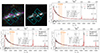 |
Fig. 1. NIRCam imaging, NIRSpec/PRISM spectroscopy, and the spectro-photometric fit for the bright LAE HCM 6A at z = 6.5676. Top left: Red-green-blue (RGB) composite image of the system constructed from JWST/NIRCam 20 mas imaging by assigning F200W to the red channel, F150W to the green channel, and F115W to the blue channel. Middle left: NIRCam F115W image of the system. The three adjacent NIRSpec slits (S1, S2, and S3) are overlaid on the RGB and F115W images targeting the three main clumps, C1–C3. Clumps C1 and C3 exhibit internal substructure and are composed of mini-clumps (C1a–C1b and C3a–C3e), ordered from brightest to faintest in the RGB image. Top-right and bottom panels: Slit-level photometry (teal circles), photometry-rescaled NIRSpec PRISM slit spectroscopy (black line), and the slit-level spectro-photometric fit using customized BAGPIPES (red line). Solid and dashed vertical lines indicate detected and undetected UV–optical emission lines, respectively. The vertical orange strip indicates the wavelength range of the UV bump absorption feature. The reduced chi-square, χν2, for each fit is shown in the top right. Insets: Basic galaxy properties derived from the SED fitting. |
2.4. Previous multiwavelength observations of HCM 6A
HCM 6A is a well-known, clumpy, and luminous LAE at z = 6.5676 behind the lensing cluster Abell 370 (Hu et al. 2002; Chary et al. 2005; Boone et al. 2007; Kanekar et al. 2013; Fuller et al. 2020). This lensed source (with lensing magnification μ ≈ 8.3 − 9.1) was first identified as an LAE candidate using Keck Low Resolution Imaging Spectrometer (LRIS) imaging and subsequently spectroscopically confirmed with LRIS (Hu et al. 2002). Its bright Lyα emission shows a strongly asymmetric profile with a steep blue cutoff, consistent with scattering in a neutral medium. Star formation rate estimates span ∼2 − 40 M⊙ yr−1, depending on whether they are derived from Lyα or UV continuum luminosity (LUV = 2 × 1029 erg s−1 Hz−1). Next, HCM 6A has also been spectroscopically confirmed with Keck Deep Imaging Multi-Object Spectrograph (DEIMOS; Fuller et al. 2020). Parameters derived from the Lyα emission line measurements from Hu et al. (2002) and Fuller et al. (2020) are reported in Table 1.
Parameters derived from the Lyα emission line measurements from the literature.
HCM 6A has also been detected with Spitzer Infrared Array Camera (IRAC) at 3.6 and 4.5 μm tracing rest-frame optical emission (Chary et al. 2005). From the Hα flux, an SFR estimate of > 140 M⊙ yr−1 is inferred – higher than estimates based on Lyα and UV, consistent with the dust extinction of AV ∼ 1. They estimated a stellar mass of M* = 8.4 × 10⁸ M⊙.
Millimeter observations of HCM 6A with the Institut de Radioastronomie Millimétrique (IRAM) 30M and NOrthern Extended Millimeter Array (NOEMA) resulted in a non-detection of the C II 158 μm and the continuum emission (Boone et al. 2007; Kanekar et al. 2013). The estimated upper limit on the dust mass is Mdust < 5.3 × 10⁷ M⊙ (Boone et al. 2007). HCM 6A has also been observed with Atacama Large Millimeter/submillimeter Array (ALMA) Band 6 (2018.1.00035.L; PI Kotaro Kohno; Fujimoto et al. 2024), at the edge of the map where the sensitivity is relatively low, resulting in a non-detection, with a 3σ upper limit of ∼0.3 mJy, corresponding to a de-lensed dust mass upper limit of Mdust ≲ 5 × 10⁶ M⊙ (following the methodology of Dunne et al. 2000; Casey 2012; Casey et al. 2014). Finally, Chandra did not detect an X-ray counterpart to HCM 6A (Bautz et al. 2000), suggesting the absence of a strong active galactic nucleus.
3. Methodology
3.1. Lyα mapping
We applied SLEUTH (Estrada-Carpenter et al. 2024, 2025) to the NIRISS WFSS spectrum with the F090WN filter (Sect. 2.1) to derive a high-quality Lyα emission line map of the LAE. SLEUTH is a spatially resolved grism-modeling pipeline that produces clean emission-line maps, accounting for spatially varying stellar populations. SLEUTH segments each galaxy into small regions – grown from the brightest pixel through nearest-neighbor expansion, until a target S/N of 20 is achieved, yielding roughly 30 regions across the source. For each region, SLEUTH forward-models spectral templates, including emission lines, and fits them to the observed grism spectra. The method explicitly captures spatial variations in stellar populations and line strengths while minimizing continuum leakage.
The extracted Lyα emission map was PSF-matched to the NIRCam/F115W resolution and resampled to a pixel scale of 0.04″. At the source’s redshift, this corresponds to ≈75 pc per pixel for an isotropic magnification of ∼8.3 − 9.1. However, the true source-plane resolution is anisotropic: ≈25 pc in the tangentially magnified direction (with μtan ≈ 7.6 − 8.4) and ≈180 pc in the radial direction (μrad ≈ 1.1). To complement the Lyα map, we extracted a 1D NIRISS spectrum from the GR150C and GR150R grisms, crossed with the four wide-band filters (F090WN–F200WN). The Lyα emission line is clearly visible at λobs ≈ 9200 Å, fully consistent with a redshift of z ≈ 6.6 (Fig. 2).
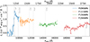 |
Fig. 2. NIRISS 1D slitless spectrum of HCM 6A. The spectrum combines extractions from the NIRISS GR150C and GR150R grisms crossed with the F090WN, F115WN, F150WN, and F200WN filters. The spectrum shows a clear detection of the Lyα emission line at λobs ≈ 9200 Å, consistent with z ≈ 6.6 (solid vertical line). Dashed vertical lines indicate the expected positions of selected undetected emission lines. |
3.2. Gravitational lens modeling and size measurements
The lens model was constrained using the parametric lens modeling code Lenstool (Kneib et al. 1996; Jullo et al. 2007). We adopted the lens model parameterization described in Gledhill et al. (2024). We further improved the model by incorporating a newly identified and confirmed multiple-image system at z = 5.97, thereby constraining the model using a catalog of 119 multiple images. The updated lens model will be available on MAST1. The magnification of the LAE, derived from the Bayesian samples of this model, lies in the range μ ≈ 8.3 − 9.1 across the source (i.e., NIRSpec slits). Most of this magnification arises from tangential stretching along the east–west direction, with a tangential component of μtan ≈ 7.6 − 8.4.
We measured the source and individual clump sizes directly in the source plane by forward-modeling the observed photometry with Lenstruction (Yang et al. 2020). The galaxy is modeled with a multicomponent profile comprising a Sérsic function for the underlying stellar component and the largest clump, and Gaussian profiles for the remaining individual clumps. The intrinsic source model is then iteratively mapped to the image plane using the gravitational-lensing maps and convolved with the empirical PSF. For the entire source, we obtain a source-plane half-light radius of 66.0 ± 0.3 milliarcseconds (mas), corresponding to ≈360 pc at z = 6.5676. The largest clump (C1a) has a best-fit size of 6.39 ± 0.2 mas (≈35 pc). However, the quoted uncertainties are likely underestimated; the true statistical uncertainties are expected to be at the ≈10 − 20% level, depending on the adopted model. All the remaining clumps are unresolved, with 2σ upper limits of < 2.8 mas (< 15 pc) on their intrinsic sizes.
3.3. SED fitting with customized BAGPIPES
Building on previous works (Markov et al. 2023, 2025a,b), we have established a robust SED fitting framework capable of simultaneously constraining galaxy physical properties and the shape of the dust attenuation curve. We applied our customized BAGPIPES SED-fitting pipeline (Markov et al. 2023) to perform joint spectro-photometric fits and infer the global (∼1 kpc), slit-level (∼0.1 kpc), and pixel-level (≈25 pc) properties of our LAE source at z = 6.5676, including stellar mass (M*), SFR (both corrected for the local lensing magnification μ), mass-weighted stellar age ( ), ionization parameter (log U), metallicity (Z), and the V-band attenuation (AV), along with the parameters (c1 − c4) of the dust attenuation model (Li et al. 2008).
We modeled galaxy spectra using a customized version of the BAGPIPES SED fitting code (Carnall et al. 2018), which employs a Bayesian framework with the MultiNest sampler (Feroz et al. 2019). Stellar emission was generated with the Stellar Population Synthesis (SPS) models of Chevallard & Charlot (2016), while nebular continuum and line emission were taken from precomputed CLOUDY grids (Ferland et al. 2017), with varying stellar age, metallicity, and ionization parameter. Our fiducial star formation history (SFH) adopts a nonparametric continuity prior (Leja et al. 2019), which provides greater flexibility and minimizes biases compared to simple parametric forms. Our customized BAGPIPES (Markov et al. 2023) includes a flexible dust attenuation law (Li et al. 2008), which captures the expected diversity of attenuation curves at high redshift (e.g., Markov et al. 2025a,b). This formalism allows both the slope and the UV bump strength to vary, enabling us to explore departures from fixed empirical dust laws. The priors and their limits for each parameter of the SED fitting model are given in Table 2.
SED fitting parameters and their priors.
We note that, although the spectroscopic redshift is securely determined from multiple emission lines, we allowed the redshift parameter in BAGPIPES to vary within a narrow prior of zspec ± 0.01. This was not intended to redetermine the redshift, but to allow limited flexibility to account for small mismatches between the low-resolution PRISM spectra and the model wavelength sampling. Fixing the redshift to zspec yields physical parameters fully consistent within the quoted uncertainties.
The analytical form of the dust attenuation model is given by
![Mathematical equation: $$ \begin{aligned} A_{\lambda }/A_V =&\frac{c_1}{(\lambda /0.08)^{c_2} +(0.08/\lambda )^{c_2} +c_3}\nonumber \\&+ \frac{233[1-c1/(6.88^{c_2}+0.145^{c_2}+c_3) -c_4/4.60]}{(\lambda /0.046)^2+(0.046/\lambda )^2+90}\nonumber \\&+ \frac{c_4}{(\lambda /0.2175)^2+(0.2175/\lambda )^2-1.95}, \end{aligned} $$](/articles/aa/full_html/2026/04/aa58580-25/aa58580-25-eq6.gif) (1)
(1)
where c1 − c4 are dimensionless parameters and λ is the wavelength in μm. The three Drude-like components on the right-hand side of Eq. (1) model, respectively, the far-UV rise, the optical–near-IR attenuation, and the ∼2175 Å bump.
For consistency with previous works (Markov et al. 2025a,b) and to facilitate comparison with literature results, we adopted the attenuation curve parameterization of Salim & Narayanan (2020), which describes each curve in terms of two key quantities: the UV–optical slope (S) and the UV bump strength (B) at ∼2175 Å. The slope, S, is defined as S = A1500/AV, where A1500 and AV are attenuation at λ = 1500 Å and in the V band, respectively. The UV bump strength, B is defined as B = Abump/A2175, where Abump denotes the excess attenuation above the baseline attenuation (i.e., the attenuation in the absence of the bump at λ = 2175 Å, and A2175 is the total attenuation at λ = 2175 Å.
To derive the global physical properties of the galaxy on kiloparsec scales, we performed SED fitting using the total HST+NIRCam photometry of the entire system. We used the catalog COLOR03 aperture fluxes and scaled them to approximate total fluxes using the KRON/COLOR03 flux ratio measured in the F277W band. This scaling ensures consistent total-flux normalization across all bands, while preserving the high-S/N colors required for reliable global SED constraints.
Next, to derive spatially resolved constraints on key physical properties, we carried out spectro-photometric SED fitting by combining the NIRSpec/PRISM spectra (reduced with msaexp v4; Brammer 2023b) with matching HST + NIRCam photometry extracted over the same aperture. NIRSpec slit has a width of 0.2″, corresponding to ∼0.37 kpc in the source plane, or ∼0.13 kpc along the tangential direction (given a magnification μ ≈ 8.3 − 9.1). Each spectrum was rescaled with corresponding photometry to correct for slit losses and ensure consistent flux calibration. In this procedure, the photometric bands with S/N < 2 and rest-frame wavelengths λrest ≲ 1300 Å were excluded to avoid contamination from Lyα emission and the damping wing region. Synthetic photometry was generated by convolving the spectra with the filter transmission curves using Dense Basis (Iyer et al. 2019). The ratio of observed to synthetic photometry was fit with a first-degree Chebyshev polynomial to derive a linear spectral correction, preventing the artificial introduction of a UV bump around λ ∼ 2175 Å.
The rescaled spectra were then masked in regions of negative flux and blueward of Lyα to remove noisy slit-edge data and possible IGM absorption. The resulting photometry, spectroscopy, and best-fit SED models for the three slits are shown in Fig. 1 (top-right and bottom panels).
Finally, we performed pixel-level SED fitting using 19-band HST + NIRCam imaging to derive spatially resolved properties on a pixel scale of 0.04″, corresponding to ≈25 pc in the source plane, owing to lensing. We restricted the analysis to pixels with S/N > 10 in the χmean detection image, which combines multiple bands weighted by their depth to optimize source detection across the field (see Sarrouh et al. 2026 for details). In addition, for this part of the analysis, we adopted a physically motivated logarithmic metallicity prior of Z/Z⊙ ∈ [0.001, 1], given the limited sensitivity of low-S/N, broadband photometry to infer Z, ensuring physically plausible solutions. Together, these complementary analyses provide a robust cross-validation of the LAE’s physical properties inferred from SED fitting across multiple spatial scales – global (∼1 kpc), slit-level (∼0.13 kpc), and pixel-level (∼25 pc).
3.4. AV from Balmer decrement and UV slope (β)
We derived the UV slope (β) values using the msaexp package (Brammer 2022, 2023b; Heintz et al. 2024; de Graaff et al. 2025) by fitting a power law to the photometry corrected NIRSpec/PRISM spectra in the rest-frame UV, specifically within the two wavelength windows: 1400 − 1860 Å and 1955 − 2580 Å, selected to avoid contamination from the C III] emission line. We also estimated the dust attenuation AVB from the Balmer decrement, defined as the ratio of the observed to intrinsic Hα/Hβ line fluxes. The observed Hα/Hβ ratios: Hα/Hβobs = 2.9 ± 0.6 for S1, Hα/Hβobs = 2.3 ± 0.4 for S2, and Hα/Hβobs = 2.3 ± 0.2 for S3; were measured from our emission line fits following the methodology of Tripodi et al. (2025). The intrinsic ratio (Hα/Hβint ≃ 2.78) was derived using the PyNeb software package (Luridiana et al. 2015), assuming an electron temperature of Te− ≃ 15 000 K and an electron density of ne− = 1000 cm−3 (Strom et al. 2017; Sanders et al. 2024).
4. Results and discussion
4.1. Global properties
We derived the global physical properties of the galaxy by fitting the total combined HST+NIRCam photometry, obtaining SFR and M* (μ-corrected), specific SFR (sSFR),  , log U, Z, AV, along with attenuation curve parameters S and B (following the parametrization of Salim & Narayanan 2020). Additionally, we estimated the intrinsic UV luminosity of the system, using the total flux in the F115W band, which closely probes the rest-frame ∼1500 Å continuum at z = 6.5676. The measured flux of fν = 0.446 ± 0.019 μJy corresponds to an observed absolute magnitude of
  . After correcting for the lensing magnification (μ = 8.3 − 91, the intrinsic UV luminosity of the galaxy is MUV = −19.8 ± 0.1, consistent with the estimate reported by Fuller et al. (2020). The intrinsic UV magnitude corresponds to a monochromatic luminosity of Lν = 3.6 ± 0.2 × 1028 erg s−1 Hz−1, a factor of ∼5 lower than the estimate by Hu et al. (2002). This luminosity is typical of moderately luminous galaxies at the EoR (e.g., Ono et al. 2010; Witstok et al. 2024, 2025; Willott et al. 2025). Global physical properties of HCM 6A are reported in Table 3.
Constrained global properties of HCM 6A.
4.2. Slit-level properties
We performed joint spectro-photometric fitting, combining HST and NIRCam slit-level (∼0.37 kpc in the source plane, or ∼0.13 kpc tangentially) photometry with photometry-rescaled NIRSpec PRISM spectra obtained in three adjacent slits (S1–S3) roughly centered on the three main clumps (C1–C3; Fig. 1). This mini-integral field unit (IFU) configuration provides slit-level, spatially resolved key physical properties from the SED fits: SFR and M* (μ-corrected),  , log U, Z, AV, along with attenuation curve parameters.
The de-lensed stellar masses are log M* = 8.04 ± 0.10 for S1, log M* = 7.75 ± 0.03 for S2, and log M* = 7.51 ± 0.02 for S3. The combined intrinsic stellar mass of the three slit regions, log M* = 8.30 ± 0.06, is in excellent agreement with the total unlensed stellar mass inferred from the integrated HST+NIRCam photometry (log M* ≃ 8.3 − 8.4; Table 3).
In addition, we independently estimated the slit-level dust attenuation from the Balmer decrement (AVB) derived from the Hα/Hβ ratio. We measured the UV continuum slope β directly from the photometry-rescaled NIRSpec spectra. These complementary estimates allowed us to cross-check and compare the attenuation inferred from the SED fitting (AV) with those derived from nebular emission lines (AVB) and from the stellar continuum (β). Figure 3 depicts slit-level, spatially resolved stellar, nebular, and dust properties across our target galaxy. The metallicity map is omitted, as SED fitting may not provide reliable constraints. However, the fitted values span Z ∼ 0.2 − 0.7 Z⊙ from the young, low-mass region (S3) to the more evolved one (S1).
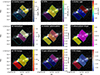 |
Fig. 3. Slit-level, spatially resolved physical properties of the target system: stellar mass (log M*; panel a), SFR (panel b), mass-weighted stellar age ( |

The AV estimates from SED fitting indicate that all three slit regions are moderately dusty (AV ∼ 0.2 − 0.4), with S3 being the most attenuated (AV ∼ 0.39 ± 0.05; Fig. 3e). In contrast, attenuation derived from the Balmer decrement (AVB) suggests a possible mild attenuation in S1 (AVB = 0.15 ± 0.70) and negligible attenuation in the remaining two regions (AVB ∼ 0; Fig. 3h), although the associated uncertainties are large. Indeed, the attenuation derived from Balmer line ratios in S2 and S3 is slightly negative (AVB ≲ 0), which is unphysical. Such results are occasionally observed, particularly in low-mass, high-redshift galaxies (e.g., Matharu et al. 2023; Shapley et al. 2023). They are likely due to measurement uncertainties or deviations in gas temperature and density from the standard Case B recombination assumptions (Osterbrock & Ferland 2006).
While S1 appears moderately dusty across all attenuation indicators, the remaining two regions show a clear tension between the stellar and nebular dust probes. The discrepancy between the V-band attenuation derived from the SED modeling (AV) and that inferred from Balmer line ratios (AVB) – most notably in S3 – may point to a complex geometry between stars, gas, and dust, where the stellar and nebular components are subject to different levels of dust obscuration (e.g., Finkelstein et al. 2008). Since AV primarily traces attenuation of the UV–optical continuum, it is intrinsically more sensitive to stellar than to nebular line emission. This interpretation is also supported by the UV continuum slope, β, which also traces dust attenuation of the stellar populations. S3 exhibits the reddest UV slope (β = −2.1 ± 0.1), corresponding to moderate stellar obscuration (AV ≳ 0.15; assuming the Meurer et al. 1999 relation), while S1 and S2 show bluer slopes (β ∼ −2.3; Figs. 3i and A.1), consistent with negligible stellar attenuation (AV ≳ 0.0). These results reinforce the interpretation that S3 experiences the highest stellar attenuation among the three regions.
In contrast, the Balmer-derived attenuation, AVB – which primarily traces dust affecting nebular emission lines – indicates a weak attenuation in S1, with AVB ∼ 0.15 (although with large uncertainty) and no significant attenuation of the ionized gas in S2 and S3, with AVB ∼ 0. This interpretation is further supported by the strength of the UV and optical emission lines in the NIRSpec PRISM spectra across the three clumps (Figs. 1 and A.1). Notably, S3 exhibits the brightest nebular emission lines (Fig. 1; bottom-right panel, Fig. A.1, insets). The potential presence of Lyα, which is particularly sensitive to resonant scattering and dust absorption (e.g., Dijkstra 2014), reinforces the conclusion that the nebular regions in S3 experience little to no dust attenuation.
We note that a tentative detection (S/N of ∼4) of the Lyα emission line is seen in the v3 NIRSpec reduction of the S3 region, whereas it is not significantly detected in v4. These two reductions correspond to independent background subtraction strategies, and the difference between the resulting v3 and v4 spectra likely reflects reduction-dependent background treatment (see Appendix B). Repeating the full analysis with the v3 spectra yields results consistent within 1−2σ, including the AVB values inferred from the Balmer decrement.
This is consistent with a very young stellar population ( Myr; Fig. 3c) and high sSFR in S3 (sSFR ≃ 55 Gyr−1) suggesting that radiation-driven outflows from a recent starburst may have cleared out much of the dust from the ionized regions (e.g., Tsuna et al. 2023; Ferrara et al. 2023; Ferrara 2024; Nakazato & Ferrara 2025). The extreme inferred sSFR in S3 places this region in a regime consistent with a super-Eddington starburst, in which feedback is expected to be dominated by radiation pressure. In this scenario, efficient dust clearing by the outflow is naturally expected, a condition also indirectly required by the detection of Lyα emission (Ferrara 2024; Nakazato & Ferrara 2025). The properties of S3 therefore closely resemble those predicted by attenuation-free models for compact, rapidly growing systems, making it a compelling analog of the “super-early” blue star-forming galaxies inferred at z ≳ 10 (Ferrara 2024; Ferrara et al. 2025; Nakazato & Ferrara 2025).
The Lyα-emitting clump (2σ contours in Fig. 4) has an observed size of 0.08″ × 0.10″, which, after correcting for lensing, corresponds to an effective source-plane radius of Reff ∼ 80 pc – combined with the young stellar age ( Myr), this yields a minimal characteristic clearing velocity of
  km s−1. This quantity represents the minimum expansion rate required to remove or dilute dust and neutral gas over the extent of the Lyα cavity. This is consistent with modest (a few tens of km s−1) local radiation- and stellar-feedback models, which predict low-velocity expansion of ionized cavities capable of opening the low-opacity channels necessary for Lyα escape (e.g., Dijkstra & Loeb 2008; Kimm et al. 2018).
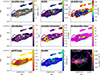 |
Fig. 4. Pixel-level, spatially resolved physical properties of the target system: stellar mass (log M*; panel a), SFR (panel b), mass-weighted stellar age ( |

In summary, the more massive, star-forming and the oldest (Figs. 3a–3c) region S1 appears moderately dusty across all attenuation indicators – suggesting a relatively uniform and more settled ISM geometry, expected for an evolved (∼240 Myr) region. In contrast, the youngest region S3 shows clear tensions between the different attenuation diagnostics, while S2 represents an intermediate case. These tensions likely reflect the various physical components probed by each diagnostic – with AV and β tracing stellar continuum attenuation, and AVB and emission line brightness tracing the nebular component – suggesting a complex dust geometry and more turbulent ISM in S3. However, the limited spatial resolution of the slit-level spectro-photometric data (∼0.1 kpc) restricts our ability to resolve the small-scale structures and disentangle these components.
4.3. Pixel-level properties
To test the geometry-driven explanation for the observed dust attenuation discrepancies, we investigated the spatially resolved properties on a pixel scale by performing SED fitting of the 19-band photometry from HST and JWST. The strong lensing magnification (μ ≈ 8.3 − 9.1) allowed us to probe extremely fine spatial scales, with the drizzled NIRCam pixel size of 0.04″ corresponding to an average of ≈25 pc in the source plane. This resolution approaches the scale of individual giant H II regions and massive star-forming clumps (e.g., Hunt & Hirashita 2009), enabling a detailed view of the galaxy’s internal structure and the interplay between dust, stars, and feedback.
On identical physical scales, we also leveraged NIRISS WFSS observations to generate a spatially resolved Lyα emission map (Fig. 4i), providing additional insight into the spatial distribution of ionized gas and its relationship with dust attenuation on ≈25 pc scale. We measure a total integrated Lyα flux of FLyα = (7.0 ± 0.3)×10−17 erg s−1 cm−2 across the entire galaxy (see Appendix B). After correcting for lensing magnification (μ ≈ 8.3 − 9.1), this corresponds to an intrinsic flux in the range of FLyα = 8.2 − 9.0 × 10⁻¹⁸ erg s−1 cm−2, depending on the magnification (μ ≈ 8.3 − 9.1), consistent with previous measurements in the literature (Hu et al. 2002; Fuller et al. 2020; see Table 1).
The spatially resolved pixel-level stellar, nebular, dust, and Lyα maps of our LAE are shown in Fig. 4. The properties log M*, SFR, and fLyα are corrected for lensing magnification based on the (World Coordinate System (WCS)-matched) magnification map, derived from the best-fit lens model, covering the region around the target galaxy. The sum of the intrinsic stellar masses over all SED-fitted pixels within the source yields log M* ≃ 9.1, a factor of ∼5 − 6 higher than the total stellar mass inferred from the integrated photometry (log M* = 8.3 − 8.4) or from the sum of the three NIRSpec slit regions (log M* ≃ 8.3). Restricting the sum to only the pixels within the three slits reduces the discrepancy, but still produces log M* ≃ 8.8, i.e., a factor of ∼3 higher than the integrated and slit-based stellar mass estimates. This discrepancy is consistent with the well-known tendency of unresolved SED-based estimates to yield systematically lower stellar masses than resolved, pixel-by-pixel SED fitting, possibly due to the outshining effect (Sorba & Sawicki 2015, 2018; Giménez-Arteaga et al. 2023; Harvey et al. 2025).
Most of the pixel-level quantities show good overall agreement with the slit-level results (Fig. 3), although the higher resolution of the pixel-based analysis reveals finer spatial variations. The main exception is the mass-weighted stellar age, which does not show consistent trends between the two approaches (Figs. 3c and 4c) – likely due to the limited ability of photometry-only SED fitting to constrain stellar ages (Chaves-Montero & Hearin 2020; Nersesian et al. 2024, 2025), given the age–dust–metallicity degeneracies (see, e.g., Walcher et al. 2011 for a review). Overall, while pixel-level SED fitting enhances spatial resolution, the accuracy of parameters, such as stellar age, metallicity, dust attenuation, and UV slope (β), remains limited by the low-S/N photometry and lack of spectroscopic coverage in individual pixels (Saxena et al. 2024; Nersesian et al. 2025). In particular, Balmer-line attenuation (AVB) requires robust spectroscopic detections of the Hα and Hβ lines.
NIRISS Lyα emission line map shows that the Lyα emission is concentrated in clump C3, with its peak located around and slightly north of the C3b mini-clump (Fig. 4i). The V-band attenuation (AV) also peaks around C3, consistent with the slit-level results (Figs. 3e and 4e), seemingly at odds with expectations given the strong sensitivity of Lyα to scattering and absorption by dust (e.g., Haiman & Spaans 1999). However, the pixel-level maps provide a more detailed view of the spatial distribution: the Lyα emission is concentrated in the central region of C3, whereas the AV peaks in the regions surrounding the Lyα peak, toward the C3 outskirts (AV ∼ 0.3 − 0.5). This spatial configuration suggests a complex ISM geometry in which the central region of C3 is largely ionized and relatively dust-free (AV ∼ 0.1 − 0.3), allowing Lyα photons to escape through cleared channels (e.g., Atek et al. 2008) even through the partially neutral IGM (e.g., Ferrara 2024). The inferred young age of this region ( Myr in S3; Fig. 3c) indicates a recent star-formation episode that has likely expelled and/or destroyed much of the dust in the core through radiation-driven outflows, displacing it toward the periphery of the clump, possibly via radiation-driven outflows (e.g., Ferrara 2024; Nakazato & Ferrara 2025). We note, however, that we are probably observing a relatively dust-cleared sightline toward the C3 core; from other orientations, dust in the outskirts could obscure the central emission and suppress the observed Lyα escape. Finally, these results also show that the presence of dust does not necessarily inhibit Lyα escape: instead, the detailed geometry of dust and stars-likely sculpted by stellar feedback-plays a determining role in regulating Lyα transmission.
4.4. Attenuation curve properties
In Fig. 5 we show the attenuation curves reconstructed from the flexible dust model parameters (c1 − c4; Li et al. 2008) implemented in our customized BAGPIPES framework (Markov et al. 2023). From the global SED fit (Table 3) to the combined photometry and rescaled NIRSpec spectra of the three slit regions (Fig. 5), the inferred attenuation curves are predominantly flat and largely featureless – i.e., “Calzetti-like” (Calzetti et al. 2000) – consistent with recent high-z observations (z ∼ 6.3 − 11.5; Markov et al. 2025a) and predictions (z ∼ 6; Narayanan et al. 2018) indicating dust dominated by large, supernova-produced grains with limited ISM reprocessing (e.g., Markov et al. 2025a; McKinney et al. 2025). Nevertheless, a measurable variation in slope and UV-bump strength can be observed across the clumps.
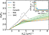 |
Fig. 5. Dust attenuation curves of the three slit regions (S1–S3) at z = 6.5676 derived from the slit-level spectro-photometric fits. S1, S2, and S3 are shown as solid blue, dashed orange, and solid green lines, respectively. Standard Milky Way (MW), Calzetti, and Small Magellanic Cloud (SMC) attenuation curves are overplotted for comparison (dashed, dotted, and solid gray lines, respectively). Inset: Corresponding SFHs of the three slit regions. |
At the slit level, the attenuation curve slope (S) remains relatively constant (S ∼ 2.3 − 2.6; Fig. 3f) across the three clumps, varying by ∼10%. Given this limited variation, we refrained from over-interpreting potential trends involving S. In contrast, the UV bump strength (B) varies more (Fig. 3g), ranging from being negligible in S3 to being more prominent in S1 and S2. Notably, B increases with decreasing AV (Fig. 3e) and increasing age (Fig. 3c), consistent with the global trends observed in, for example, Battisti et al. (2020) and Markov et al. (2025b).
We report a tentative (∼2.6σ) detection of a weak UV bump in the slit region S1 of the LAE, with the UV bump parameter c4 = 0.012 ± 0.005 (B = 0.10 ± 0.05), corresponding to ∼23% (∼28%) of the Milky Way bump. To confirm the presence of the 2175 Å UV bump in this source, we used χ2 statistics (e.g., Lucy 2016) to perform a nested model comparison between (i) the fiducial SED model (with a free UV bump amplitude c4) and (ii) the same model without a bump (with c4 = 0). The comparison yields only weak evidence for the presence of the feature in the spectral region around the bump (p ≃ 0.25), whereas the full-spectrum fit shows a significant improvement when including the bump component (p < 0.05).
At the pixel level, both the dust attenuation curve slope (S) and UV bump amplitude (B) exhibit a broader range of variation compared to the slit-level results (panels f and g of Figs. 3 and 4). In addition, both S and B peak around the position of clump C1 (C1a), extending slightly toward C2, with a smaller peak around the C3e mini-clump (Figs. 3f and 3g). The SFR (averaged over 10 Myr), sSFR, and ionization parameter (log U; Figs. 3b, 3i, and 3d, respectively) also peak between and northward of C1 and C2, with smaller peaks around C3d-e, potentially tracing merger-induced recent star formation. The resulting strong radiation fields in these regions may drive the reprocessing of dust grains and the production of smaller grains (including carbonaceous grains or polycyclic aromatic hydrocarbons), leading to steeper slopes and stronger UV bumps (Narayanan et al. 2023; Ormerod et al. 2025).
This behavior contrasts with trends typically observed on global galaxy scales, where steeper slopes and stronger bumps are typically associated with lower sSFRs and older stellar populations (e.g., Kriek & Conroy 2013; Battisti et al. 2020; Markov et al. 2025b). This discrepancy likely reflects the different drivers of the sSFR on local versus global scales: globally, the sSFR is driven mainly by the inverse of stellar age (e.g., Langeroodi et al. 2024) or stellar mass (by definition); locally, sSFR variations arise mostly from local variations in SFR at nearly fixed stellar mass within a single clump (Fig. 4). As a result, the pixel-level correlation between S, B, and SFR (sSFR) probably traces spatially localized star formation and feedback, whereas the global anticorrelation with sSFR reflects longer-term evolutionary trends.
5. Summary and conclusions
We have presented a detailed case study of the well-known, strongly lensed Lyα-emitting galaxy HCM 6A at z = 6.5676, located behind Abell 370 and observed as part of JWST/CANUCS. Combining 19-band HST+NIRCam photometry, three JWST/NIRSpec slits, and NIRISS imaging and slitless spectroscopy, we constrained the galaxy’s Lyα emission, spatially resolved physical properties, and dust attenuation curve. A high-quality Lyα map from SLEUTH further revealed the spatial distribution of Lyα emission. Using a customized BAGPIPES SED-fitting framework with a flexible dust law, we derived stellar, nebular, and dust properties across multiple spatial scales – from integrated (≈1 kpc) to slit (≈0.1 kpc) and pixel levels (down to ≈25 pc tangentially) – enabled by strong lensing magnification (μ ≈ 8.3 − 9.1).
Together, these multiwavelength, spatially resolved observations provide an unprecedented view of the interplay between dust, Lyα escape, and feedback in a clumpy galaxy near the end of reionization. Our main results are:
-
From integrated HST+NIRCam photometry, we infer an unlensed stellar mass of log M* = 8.3 − 8.4, consistent with the sum of the de-lensed masses of the three NIRSpec slit regions. Using the F115W continuum, which traces the rest-frame UV at 1500 Å, we measure an intrinsic UV magnitude of MUV = −19.8 ± 0.1, corresponding to a luminosity of Lν = 3.6 × 1028 erg s−1 Hz−1.
-
Slit-level (≈0.1 kpc) maps show that the most massive, oldest region, S1, is moderately dusty and consistent across all attenuation indicators, suggesting a uniform ISM geometry. In contrast, the youngest region, S3, shows strong discrepancies between stellar (AV, β) and nebular (AVB, line emission) tracers, indicating a complex, multiphase dust geometry, possibly shaped by recent feedback.
-
The pixel-level, NIRISS Lyα emission line map shows that Lyα emission arises mainly from clump C3, where AV is also high on average. Pixel-level maps reveal that Lyα emerges from the dust-cleared core, while AV peaks in the clump outskirts. This is consistent with a possible recent starburst (
 Myr) that ionized the core and expelled dust via radiation-driven outflows, enabling Lyα escape through low-opacity channels.
 -
We constructed one of the first spatially resolved attenuation curve maps at z > 6. Slit-level measurements yield a broadly Calzetti-like slope (S ≈ 2.3 − 2.6) and a UV bump strength (B) that increases with stellar age and lower AV. Pixel-level maps show that both S and B rise in the more evolved region between clumps C1 and C2, consistent with dust-grain processing and the formation of small (carbon-rich) grains in a star-forming region.
-
We find weak evidence (∼2.6σ) for a UV bump in S1 (∼25% of the Milky Way bump).
These findings provide the spatially resolved view of HCM 6A down to ≈25 pc, revealing how dust, gas, and stars interacted within a moderately dusty LAE at the EoR. Our combination of slit-level photometry and spectroscopy, together with pixel-level photometry and Lyα mapping, reveals a complex, multiphase ISM shaped by recent star formation and feedback, and demonstrates that low-opacity channels enable Lyα escape. Importantly, these results show that dust does not necessarily suppress Lyα escape; instead, the small-scale geometry of dust and stars – likely reshaped by recent feedback – plays a central role in regulating Lyα transmission.
However, our knowledge of some key physical quantities – such as AVB, gas-phase metallicity, and ionization state – remains limited by the lack of fully resolved spectroscopy, while parameters like stellar age, attenuation, and β remain uncertain due to the low S/N at the pixel level. Future deep JWST/NIRSpec IFU observations can overcome these limitations by providing spatially resolved spectroscopy, which enables robust measurements of the dust, gas, and ionization structure, and allows for a definitive test of the mechanisms regulating Lyα escape.
Acknowledgments
We thank the anonymous referee for their valuable comments and suggestions, which helped improve the clarity and quality of this work. We thank Johannes Zabl for detailed comments and helpful suggestions during the preparation of this manuscript. VM, MB, GR, JJ, and NM acknowledge support from the ERC Grant FIRSTLIGHT and the Slovenian National Research Agency ARRS through grants N1-0238, P1-0188. GR and MB acknowledge support from the European Space Agency through Prodex Experiment Arrangement No. 4000146646. This research was enabled by grants 18JWST-GTO1 and 23JWGO2B04 from the Canadian Space Agency. MS, VEC, GD, and GN acknowledge support from the Natural Sciences and Engineering Research Council (NSERC) of Canada through grants RGPIN-2020-06023, RGPAS-2020-00065. GN acknowledges support by the Canadian Space Agency under a contract with NRC Herzberg Astronomy and Astrophysics. AH acknowledges support by the Science and Technology Facilities Council (STFC), by the ERC through Advanced Grant 695671 “QUENCH”, and by the UKRI Frontier Research grant RISEandFALL. The authors acknowledge the use of the Canadian Advanced Network for Astronomy Research (CANFAR) Science Platform operated by the Canadian Astronomy Data Centre (CADC) and the Digital Research Alliance of Canada (DRAC), with support from the National Research Council of Canada (NRC), the Canadian Space Agency (CSA), CANARIE, and the Canadian Foundation for Innovation (CFI). This work made use of Astropy (http://www.astropy.org), a community-developed core Python package and an ecosystem of tools and resources for astronomy (Astropy Collaboration 2022).
References
- Astropy Collaboration (Price-Whelan, A. M., et al.) 2022, ApJ, 935, 167 [NASA ADS] [CrossRef] [Google Scholar]
- Atek, H., Kunth, D., Hayes, M., Östlin, G., & Mas-Hesse, J. M. 2008, A&A, 488, 491 [NASA ADS] [CrossRef] [EDP Sciences] [Google Scholar]
- Atek, H., Kunth, D., Schaerer, D., et al. 2009, A&A, 506, L1 [NASA ADS] [CrossRef] [EDP Sciences] [Google Scholar]
- Battisti, A. J., Cunha, E. D., Shivaei, I., & Calzetti, D. 2020, ApJ, 888, 108 [NASA ADS] [CrossRef] [Google Scholar]
- Bautz, M. W., Malm, M. R., Baganoff, F. K., et al. 2000, ApJ, 543, L119 [Google Scholar]
- Behrens, C., Pallottini, A., Ferrara, A., Gallerani, S., & Vallini, L. 2019, MNRAS, 486, 2197 [NASA ADS] [CrossRef] [Google Scholar]
- Bolan, P., Bradăc, M., Lemaux, B. C., et al. 2024, MNRAS, 531, 2998 [Google Scholar]
- Boone, F., Schaerer, D., Pelló, R., Combes, F., & Egami, E. 2007, A&A, 475, 513 [NASA ADS] [CrossRef] [EDP Sciences] [Google Scholar]
- Brammer, G. 2022, https://doi.org/10.5281/zenodo.7299500 [Google Scholar]
- Brammer, G. 2023a, https://doi.org/10.5281/zenodo.1146904 [Google Scholar]
- Brammer, G. 2023b, https://doi.org/10.5281/zenodo.7299500 [Google Scholar]
- Calzetti, D., Armus, L., Bohlin, R. C., et al. 2000, ApJ, 533, 682 [NASA ADS] [CrossRef] [Google Scholar]
- Carnall, A. C., McLure, R. J., Dunlop, J. S., & Davé, R. 2018, MNRAS, 480, 4379 [Google Scholar]
- Casey, C. M. 2012, MNRAS, 425, 3094 [Google Scholar]
- Casey, C. M., Narayanan, D., & Cooray, A. 2014, Phys. Rep., 541, 45 [Google Scholar]
- Chary, R.-R., Stern, D., & Eisenhardt, P. 2005, ApJ, 635, L5 [CrossRef] [Google Scholar]
- Chaves-Montero, J., & Hearin, A. 2020, MNRAS, 495, 2088 [NASA ADS] [CrossRef] [Google Scholar]
- Chevallard, J., & Charlot, S. 2016, MNRAS, 462, 1415 [NASA ADS] [CrossRef] [Google Scholar]
- Comrie, A., Wang, K. S., Hsu, S. C., et al. 2021, https://doi.org/10.5281/zenodo.3377984 [Google Scholar]
- de Graaff, A., Brammer, G., Weibel, A., et al. 2025, A&A, 697, A189 [NASA ADS] [CrossRef] [EDP Sciences] [Google Scholar]
- Desprez, G., Martis, N. S., Asada, Y., et al. 2024, MNRAS, 530, 2935 [Google Scholar]
- Dijkstra, M. 2014, PASA, 31, e040 [Google Scholar]
- Dijkstra, M., & Loeb, A. 2008, MNRAS, 391, 457 [NASA ADS] [CrossRef] [Google Scholar]
- Dunne, L., Eales, S., Edmunds, M., et al. 2000, MNRAS, 315, 115 [Google Scholar]
- Estrada-Carpenter, V., Sawicki, M., Brammer, G., et al. 2024, MNRAS, 532, 577 [NASA ADS] [CrossRef] [Google Scholar]
- Estrada-Carpenter, V., Sawicki, M., Abraham, R., et al. 2025, ApJ, 991, 188 [Google Scholar]
- Ferland, G. J., Chatzikos, M., Guzmán, F., et al. 2017, Rev. Mexicana Astron. Astrofis., 53, 385 [Google Scholar]
- Feroz, F., Hobson, M. P., Cameron, E., & Pettitt, A. N. 2019, Open J. Astrophys., 2, 10 [Google Scholar]
- Ferrara, A. 2024, A&A, 684, A207 [NASA ADS] [CrossRef] [EDP Sciences] [Google Scholar]
- Ferrara, A., Pallottini, A., & Dayal, P. 2023, MNRAS, 522, 3986 [NASA ADS] [CrossRef] [Google Scholar]
- Ferrara, A., Pallottini, A., & Sommovigo, L. 2025, A&A, 694, A286 [NASA ADS] [CrossRef] [EDP Sciences] [Google Scholar]
- Finkelstein, S. L., Rhoads, J. E., Malhotra, S., Grogin, N., & Wang, J. 2008, ApJ, 678, 655 [Google Scholar]
- Finkelstein, S. L., Rhoads, J. E., Malhotra, S., & Grogin, N. 2009, ApJ, 691, 465 [NASA ADS] [CrossRef] [Google Scholar]
- Fujimoto, S., Kohno, K., Ouchi, M., et al. 2024, ApJS, 275, 36 [NASA ADS] [Google Scholar]
- Fuller, S., Lemaux, B. C., Bradač, M., et al. 2020, ApJ, 896, 156 [NASA ADS] [CrossRef] [Google Scholar]
- Giménez-Arteaga, C., Oesch, P. A., Brammer, G. B., et al. 2023, ApJ, 948, 126 [CrossRef] [Google Scholar]
- Gledhill, R., Strait, V., Desprez, G., et al. 2024, ApJ, 973, 77 [CrossRef] [Google Scholar]
- Goovaerts, I., Pello, R., Thai, T. T., et al. 2023, A&A, 678, A174 [NASA ADS] [CrossRef] [EDP Sciences] [Google Scholar]
- Gronke, M., & Dijkstra, M. 2016, ApJ, 826, 14 [NASA ADS] [CrossRef] [Google Scholar]
- Gunn, J. E., & Peterson, B. A. 1965, ApJ, 142, 1633 [Google Scholar]
- Haiman, Z., & Spaans, M. 1999, ApJ, 518, 138 [NASA ADS] [CrossRef] [Google Scholar]
- Hansen, M., & Oh, S. P. 2006, MNRAS, 367, 979 [NASA ADS] [CrossRef] [Google Scholar]
- Harvey, T., Conselice, C. J., Adams, N. J., et al. 2025, MNRAS, 542, 2998 [Google Scholar]
- Hayes, M., Schaerer, D., Östlin, G., et al. 2011, ApJ, 730, 8 [NASA ADS] [CrossRef] [Google Scholar]
- Heintz, K. E., Watson, D., Brammer, G., et al. 2024, Science, 384, 890 [NASA ADS] [CrossRef] [Google Scholar]
- Heintz, K. E., Brammer, G. B., Watson, D., et al. 2025, A&A, 693, A60 [Google Scholar]
- Hu, E. M., Cowie, L. L., McMahon, R. G., et al. 2002, ApJ, 568, L75 [Google Scholar]
- Hunt, L. K., & Hirashita, H. 2009, A&A, 507, 1327 [NASA ADS] [CrossRef] [EDP Sciences] [Google Scholar]
- Iyer, K. G., Gawiser, E., Faber, S. M., et al. 2019, ApJ, 879, 116 [NASA ADS] [CrossRef] [Google Scholar]
- Jullo, E., Kneib, J.-P., Limousin, M., et al. 2007, New J. Phys., 9, 447 [Google Scholar]
- Kanekar, N., Wagg, J., Chary, R. R., & Carilli, C. L. 2013, ApJ, 771, L20 [NASA ADS] [CrossRef] [Google Scholar]
- Keating, L. C., Puchwein, E., Bolton, J. S., Haehnelt, M. G., & Kulkarni, G. 2024a, MNRAS, 531, L34 [Google Scholar]
- Keating, L. C., Bolton, J. S., Cullen, F., et al. 2024b, MNRAS, 532, 1646 [Google Scholar]
- Kimm, T., Haehnelt, M., Blaizot, J., et al. 2018, MNRAS, 475, 4617 [CrossRef] [Google Scholar]
- Kneib, J. P., Ellis, R. S., Smail, I., Couch, W. J., & Sharples, R. M. 1996, ApJ, 471, 643 [Google Scholar]
- Kornei, K. A., Shapley, A. E., Erb, D. K., et al. 2010, ApJ, 711, 693 [NASA ADS] [CrossRef] [Google Scholar]
- Kriek, M., & Conroy, C. 2013, ApJ, 775, L16 [NASA ADS] [CrossRef] [Google Scholar]
- Langeroodi, D., Hjorth, J., Ferrara, A., & Gall, C. 2024, Nature, submitted [arXiv:2410.14671] [Google Scholar]
- Leja, J., Carnall, A. C., Johnson, B. D., Conroy, C., & Speagle, J. S. 2019, ApJ, 876, 3 [Google Scholar]
- Leonova, E., Oesch, P. A., Qin, Y., et al. 2022, MNRAS, 515, 5790 [NASA ADS] [CrossRef] [Google Scholar]
- Li, A., Liang, S. L., Kann, D. A., et al. 2008, ApJ, 685, 1046 [NASA ADS] [CrossRef] [Google Scholar]
- Lotz, J. M., Koekemoer, A., Coe, D., et al. 2017, ApJ, 837, 97 [Google Scholar]
- Lucy, L. B. 2016, A&A, 588, A19 [NASA ADS] [CrossRef] [EDP Sciences] [Google Scholar]
- Luridiana, V., Morisset, C., & Shaw, R. A. 2015, A&A, 573, A42 [NASA ADS] [CrossRef] [EDP Sciences] [Google Scholar]
- Markov, V., Gallerani, S., Pallottini, A., et al. 2023, A&A, 679, A12 [NASA ADS] [CrossRef] [EDP Sciences] [Google Scholar]
- Markov, V., Gallerani, S., Ferrara, A., et al. 2025a, Nat. Astron., 9, 458 [Google Scholar]
- Markov, V., Gallerani, S., Pallottini, A., et al. 2025b, A&A, 702, A33 [NASA ADS] [CrossRef] [EDP Sciences] [Google Scholar]
- Martis, N. S., Sarrouh, G. T. E., Willott, C. J., et al. 2024, ApJ, 975, 76 [NASA ADS] [CrossRef] [Google Scholar]
- Maseda, M. V., Bacon, R., Lam, D., et al. 2020, MNRAS, 493, 5120 [Google Scholar]
- Mason, C. A., Treu, T., Dijkstra, M., et al. 2018, ApJ, 856, 2 [Google Scholar]
- Matharu, J., & Brammer, G. 2022, https://doi.org/10.5281/zenodo.7628094 [Google Scholar]
- Matharu, J., Muzzin, A., Sarrouh, G. T. E., et al. 2023, ApJ, 949, L11 [NASA ADS] [CrossRef] [Google Scholar]
- Matthee, J., Sobral, D., Hayes, M., et al. 2021, MNRAS, 505, 1382 [NASA ADS] [CrossRef] [Google Scholar]
- McKinney, J., Cooper, O. R., Casey, C. M., et al. 2025, ApJ, 985, L21 [Google Scholar]
- Meurer, G. R., Heckman, T. M., & Calzetti, D. 1999, ApJ, 521, 64 [Google Scholar]
- Nakazato, Y., & Ferrara, A. 2025, MNRAS, 544, 4390 [Google Scholar]
- Nakazato, Y., Matsumoto, K., Inoue, A. K., et al. 2026, ApJ, submitted [arXiv:2602.07347] [Google Scholar]
- Napolitano, L., Pentericci, L., Santini, P., et al. 2024, A&A, 688, A106 [NASA ADS] [CrossRef] [EDP Sciences] [Google Scholar]
- Narayanan, D., Conroy, C., Davé, R., Johnson, B. D., & Popping, G. 2018, ApJ, 869, 70 [Google Scholar]
- Narayanan, D., Smith, J. D. T., Hensley, B. S., et al. 2023, ApJ, 951, 100 [NASA ADS] [CrossRef] [Google Scholar]
- Nersesian, A., van der Wel, A., Gallazzi, A., et al. 2024, A&A, 681, A94 [NASA ADS] [CrossRef] [EDP Sciences] [Google Scholar]
- Nersesian, A., van der Wel, A., Gallazzi, A. R., et al. 2025, A&A, 695, A86 [NASA ADS] [CrossRef] [EDP Sciences] [Google Scholar]
- Neufeld, D. A. 1991, ApJ, 370, L85 [Google Scholar]
- Neyer, M., Smith, A., Vogelsberger, M., et al. 2025, ArXiv e-prints [arXiv:2510.18946] [Google Scholar]
- Noirot, G., Desprez, G., Asada, Y., et al. 2023, MNRAS, 525, 1867 [NASA ADS] [CrossRef] [Google Scholar]
- Noirot, G., NIRISS WFSS Team, Goudfrooij, P., et al. 2025, Global Sky Background Images for JWST/NIRISS Wide-Field Slitless Spectroscopy, Tech. Rep. Technical Report JWST-STScI-009057, STScI [Google Scholar]
- Ono, Y., Ouchi, M., Shimasaku, K., et al. 2010, ApJ, 724, 1524 [NASA ADS] [CrossRef] [Google Scholar]
- Ormerod, K., Witstok, J., Smit, R., et al. 2025, MNRAS, 542, 1136 [Google Scholar]
- Osterbrock, D. E., & Ferland, G. J. 2006, Astrophysics of Gaseous Nebulae and Active Galactic Nuclei (Sausalito: University Science Books) [Google Scholar]
- Ouchi, M., Ono, Y., & Shibuya, T. 2020, ARA&A, 58, 617 [Google Scholar]
- Partridge, R. B., & Peebles, P. J. E. 1967, ApJ, 147, 868 [Google Scholar]
- Postman, M., Coe, D., Benítez, N., et al. 2012, ApJS, 199, 25 [Google Scholar]
- Prieto-Lyon, G., Mason, C. A., Strait, V., et al. 2025, A&A, submitted [arXiv:2509.18302] [Google Scholar]
- Reddy, N. A., Kriek, M., Shapley, A. E., et al. 2015, ApJ, 806, 259 [NASA ADS] [CrossRef] [Google Scholar]
- Robertson, B. E., Ellis, R. S., Dunlop, J. S., McLure, R. J., & Stark, D. P. 2010, Nature, 468, 49 [Google Scholar]
- Salim, S., & Narayanan, D. 2020, ARA&A, 58, 529 [NASA ADS] [CrossRef] [Google Scholar]
- Salim, S., Lee, J. C., Janowiecki, S., et al. 2016, ApJS, 227, 2 [NASA ADS] [CrossRef] [Google Scholar]
- Sanders, R. L., Shapley, A. E., Topping, M. W., Reddy, N. A., & Brammer, G. B. 2024, ApJ, 962, 24 [NASA ADS] [CrossRef] [Google Scholar]
- Santos, M. R. 2004, MNRAS, 349, 1137 [NASA ADS] [CrossRef] [Google Scholar]
- Sarrouh, G. T. E., Asada, Y., Martis, N. S., et al. 2026, ApJS, 282, 3 [Google Scholar]
- Saxena, A., Cameron, A. J., Katz, H., et al. 2024, MNRAS, submitted [arXiv:2411.14532] [Google Scholar]
- Scarlata, C., Colbert, J., Teplitz, H. I., et al. 2009, ApJ, 704, L98 [NASA ADS] [CrossRef] [Google Scholar]
- Schaerer, D. 2003, A&A, 397, 527 [NASA ADS] [CrossRef] [EDP Sciences] [Google Scholar]
- Shapley, A. E., Steidel, C. C., Pettini, M., & Adelberger, K. L. 2003, ApJ, 588, 65 [Google Scholar]
- Shapley, A. E., Sanders, R. L., Reddy, N. A., Topping, M. W., & Brammer, G. B. 2023, ApJ, 954, 157 [NASA ADS] [CrossRef] [Google Scholar]
- Shipley, H. V., Lange-Vagle, D., Marchesini, D., et al. 2018, ApJS, 235, 14 [Google Scholar]
- Sorba, R., & Sawicki, M. 2015, MNRAS, 452, 235 [NASA ADS] [CrossRef] [Google Scholar]
- Sorba, R., & Sawicki, M. 2018, MNRAS, 476, 1532 [NASA ADS] [CrossRef] [Google Scholar]
- Steinhardt, C. L., Jauzac, M., Acebron, A., et al. 2020, ApJS, 247, 64 [Google Scholar]
- Strom, A. L., Steidel, C. C., Rudie, G. C., et al. 2017, ApJ, 836, 164 [NASA ADS] [CrossRef] [Google Scholar]
- Tilvi, V., Papovich, C., Finkelstein, S. L., et al. 2014, ApJ, 794, 5 [Google Scholar]
- Torralba, A., Matthee, J., Naidu, R. P., et al. 2024, A&A, 689, A44 [NASA ADS] [CrossRef] [EDP Sciences] [Google Scholar]
- Treu, T., Schmidt, K. B., Trenti, M., Bradley, L. D., & Stiavelli, M. 2013, ApJ, 775, L29 [NASA ADS] [CrossRef] [Google Scholar]
- Tripodi, R., Martis, N., Markov, V., et al. 2025, Nat. Commun., 16, 9830 [Google Scholar]
- Tsuna, D., Nakazato, Y., & Hartwig, T. 2023, MNRAS, 526, 4801 [NASA ADS] [CrossRef] [Google Scholar]
- Verhamme, A., Schaerer, D., Atek, H., & Tapken, C. 2008, A&A, 491, 89 [NASA ADS] [CrossRef] [EDP Sciences] [Google Scholar]
- Walcher, J., Groves, B., Budavári, T., & Dale, D. 2011, Ap&SS, 331, 1 [NASA ADS] [CrossRef] [Google Scholar]
- Whitler, L. R., Mason, C. A., Ren, K., et al. 2020, MNRAS, 495, 3602 [Google Scholar]
- Willott, C. J., Doyon, R., Albert, L., et al. 2022, PASP, 134, 025002 [CrossRef] [Google Scholar]
- Willott, C. J., Asada, Y., Iyer, K. G., et al. 2025, ApJ, 988, 26 [Google Scholar]
- Witstok, J., Smit, R., Saxena, A., et al. 2024, A&A, 682, A40 [NASA ADS] [CrossRef] [EDP Sciences] [Google Scholar]
- Witstok, J., Maiolino, R., Smit, R., et al. 2025, MNRAS, 536, 27 [Google Scholar]
- Yang, H., Malhotra, S., Gronke, M., et al. 2017, ApJ, 844, 171 [NASA ADS] [CrossRef] [Google Scholar]
- Yang, L., Birrer, S., & Treu, T. 2020, MNRAS, 496, 2648 [NASA ADS] [CrossRef] [Google Scholar]
Appendix A: Overplotted spectra of individual slit regions (S1–S3)
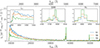 |
Fig. A.1. Photometry-rescaled NIRSpec PRISM slit spectra extracted from three adjacent slit regions (S1, S2, and S3; shown in blue, orange, and green, respectively). Main panel: Spectra as a function of observed wavelength, with the corresponding rest-frame wavelength shown on the upper axis. Insets: Zoomed-in views around the Lyα, [O III] doublet, and Hα emission-line regions (left, center, and right, respectively). Dashed vertical lines mark the expected wavelengths of the emission lines. Insets have the same spectral flux density (fλ) and observed wavelength (λobs) units as the main panel. |
Appendix B: Integrated and slit-resolved Lyα fluxes
In Table B.1 we report observed Lyα fluxes not corrected for gravitational lensing magnification, measured for the integrated system and within the three NIRSpec slit regions (S1–S3), using different methods. Column (b) lists fluxes from the NIRISS Lyα map integrated within the adopted aperture encompassing the entire source (total) and the three slits (S1-S3), using CARTA (Cube Analysis and Rendering Tool for Astronomy; Comrie et al. 2021). The sum of the map-based fluxes within S1–S3 corresponds to ≈55% of the total flux of the system, indicating that nearly half of the Lyα emission lies outside the NIRSpec apertures. This highlights that, for spatially extended Lyα emission, NIRSpec slit observations can recover only a fraction of the total flux, an effect that should be considered in large survey studies of LAEs. Column (c) reports the integrated Lyα flux derived from a direct forward-model fit to the 2D NIRISS slitless spectrum using a template-based approach with grizli, where the flux corresponds to the best-fit scaling of the Lyα template.
Lyα fluxes FLyα [×10−17 erg cm−2 s−1] or their 3σ upper limits.
Columns (d) and (e) list Lyα fluxes from fits to the photometry-rescaled 1D NIRSpec spectra (v4 and v3) using the Dawn JWST Archive (DJA) NIRSpec data products code (Heintz et al. 2024; de Graaff et al. 2025). A marginal Lyα detection (S/N ≈ 4) is present in the v3 NIRSpec spectrum of S3, while no significant line is recovered in the corresponding v4 extraction. This discrepancy originates from the reduction-dependent background treatment, potentially including self-subtraction effects in v4.
All Tables
All Figures
|
Fig. 1. NIRCam imaging, NIRSpec/PRISM spectroscopy, and the spectro-photometric fit for the bright LAE HCM 6A at z = 6.5676. Top left: Red-green-blue (RGB) composite image of the system constructed from JWST/NIRCam 20 mas imaging by assigning F200W to the red channel, F150W to the green channel, and F115W to the blue channel. Middle left: NIRCam F115W image of the system. The three adjacent NIRSpec slits (S1, S2, and S3) are overlaid on the RGB and F115W images targeting the three main clumps, C1–C3. Clumps C1 and C3 exhibit internal substructure and are composed of mini-clumps (C1a–C1b and C3a–C3e), ordered from brightest to faintest in the RGB image. Top-right and bottom panels: Slit-level photometry (teal circles), photometry-rescaled NIRSpec PRISM slit spectroscopy (black line), and the slit-level spectro-photometric fit using customized BAGPIPES (red line). Solid and dashed vertical lines indicate detected and undetected UV–optical emission lines, respectively. The vertical orange strip indicates the wavelength range of the UV bump absorption feature. The reduced chi-square, χν2, for each fit is shown in the top right. Insets: Basic galaxy properties derived from the SED fitting. |
| In the text | |
|
Fig. 2. NIRISS 1D slitless spectrum of HCM 6A. The spectrum combines extractions from the NIRISS GR150C and GR150R grisms crossed with the F090WN, F115WN, F150WN, and F200WN filters. The spectrum shows a clear detection of the Lyα emission line at λobs ≈ 9200 Å, consistent with z ≈ 6.6 (solid vertical line). Dashed vertical lines indicate the expected positions of selected undetected emission lines. |
| In the text | |
|
Fig. 3. Slit-level, spatially resolved physical properties of the target system: stellar mass (log M*; panel a), SFR (panel b), mass-weighted stellar age ( |
| In the text | |
|
Fig. 4. Pixel-level, spatially resolved physical properties of the target system: stellar mass (log M*; panel a), SFR (panel b), mass-weighted stellar age ( |
| In the text | |
|
Fig. 5. Dust attenuation curves of the three slit regions (S1–S3) at z = 6.5676 derived from the slit-level spectro-photometric fits. S1, S2, and S3 are shown as solid blue, dashed orange, and solid green lines, respectively. Standard Milky Way (MW), Calzetti, and Small Magellanic Cloud (SMC) attenuation curves are overplotted for comparison (dashed, dotted, and solid gray lines, respectively). Inset: Corresponding SFHs of the three slit regions. |
| In the text | |
|
Fig. A.1. Photometry-rescaled NIRSpec PRISM slit spectra extracted from three adjacent slit regions (S1, S2, and S3; shown in blue, orange, and green, respectively). Main panel: Spectra as a function of observed wavelength, with the corresponding rest-frame wavelength shown on the upper axis. Insets: Zoomed-in views around the Lyα, [O III] doublet, and Hα emission-line regions (left, center, and right, respectively). Dashed vertical lines mark the expected wavelengths of the emission lines. Insets have the same spectral flux density (fλ) and observed wavelength (λobs) units as the main panel. |
| In the text | |
Current usage metrics show cumulative count of Article Views (full-text article views including HTML views, PDF and ePub downloads, according to the available data) and Abstracts Views on Vision4Press platform.
Data correspond to usage on the plateform after 2015. The current usage metrics is available 48-96 hours after online publication and is updated daily on week days.
Initial download of the metrics may take a while.