| Issue |
A&A
Volume 708, April 2026
|
|
|---|---|---|
| Article Number | A65 | |
| Number of page(s) | 11 | |
| Section | Extragalactic astronomy | |
| DOI | https://doi.org/10.1051/0004-6361/202558622 | |
| Published online | 26 March 2026 | |
The supersonic nature of jellyfish galaxies
1
INAF – Osservatorio Astronomico di Padova, Vicolo dell’Osservatorio 5, 35122 Padova, (PD), Italy
2
INAF – Osservatorio Astronomico di Cagliari, Via della Scienza 5, 09047 Selargius, (CA), Italy
3
Leibniz Institute for Astrophysics Potsdam (AIP), An der Sternwarte 16, 14482 Potsdam, Germany
4
Center for Computational Astrophysics, Flatiron Institute, 162 5th Avenue, 10010 New York, (NY), USA
5
Departamento de Física, Universidad Técnica Federico Santa María, Avenida España 1680 Valparaíso, Chile
6
Millennium Nucleus for Galaxies (MINGAL), Valparaíso, Chile
7
DARK, Niels Bohr Institute, University of Copenhagen, Jagtvej 155, 2200 Copenhagen, Denmark
8
Kapteyn Astronomical Institute, University of Groningen, Landleven 12, 9747 AD, Groningen, The Netherlands
9
Department of Physics and Astronomy “Augusto Righi”, University of Bologna, Via Gobetti 93/2, 40129 Bologna, (BO), Italy
10
INAF – Osservatorio Astronomico di Brera, Via Brera 28, 20121 Milano, (MI), Italy
11
University Observatory, LMU Faculty of Physics, Scheinerstrassee 1, 81679 München, Germany
12
INAF – Istituto di Radioastronomia, Via Piero Gobetti 101, 40129 Bologna, (BO), Italy
13
INAF – Osservatorio di Astrofisica e Scienza dello Spazio Bologna, Via Piero Gobetti, 93/3, 40129 Bologna, (BO), Italy
14
Department of Physics, Faculty of Science, University of Zagreb, Bijenička 32, 10 000 Zagreb, Croatia
15
Astronomical Institute (AIRUB), Ruhr-University Bochum, Faculty of Physics and Astronomy, 44780 Bochum, Germany
★ Corresponding author: This email address is being protected from spambots. You need JavaScript enabled to view it.
Received:
17
December
2025
Accepted:
25
February
2026
Abstract
All gas-rich galaxies in cluster environments are expected to experience ram-pressure stripping from the intracluster medium. However, only a fraction of these develop ongoing star formation in their stripped tail, becoming the so-called jellyfish galaxies. In this work we provide observational evidence that magnetic fields can signal differences in extraplanar star formation, and we explore the physical conditions that lead to the formation of a jellyfish galaxy. We first focus on JO147, a jellyfish galaxy that features weak star formation activity in its tail. Using MeerKAT radio continuum observations, we discovered polarized emission only in a small fraction of its tail, with an average fraction of 10%, and a low Mach number, ℳ = 1.3 − 1.6, suggesting a possible association between magnetic field draping, shock compression of the gas, and extraplanar star formation activity. We then tested this scenario in a sample of 17 jellyfish galaxies from the GASP project. We combined dynamical models for their orbits within the host clusters with realistic cluster temperature profiles to infer their Mach number, and we found a positive correlation between it and the star formation activity in their tail. We conclude that supersonic motion is a necessary condition for triggering star formation in the stripped tails of jellyfish galaxies. Our findings provide empirical evidence that the critical factor preventing evaporation of the stripped gas is the shock compression induced by the supersonic motion through the cluster. This process likely enhances the magnetic field surrounding the galaxy and the properties of the stripped material.
Key words: magnetic fields / galaxies: clusters: general / radio continuum: galaxies
© The Authors 2026
 Open Access article, published by EDP Sciences, under the terms of the Creative Commons Attribution License (https://creativecommons.org/licenses/by/4.0), which permits unrestricted use, distribution, and reproduction in any medium, provided the original work is properly cited.
This article is published in open access under the Subscribe to Open model. This email address is being protected from spambots. You need JavaScript enabled to view it. to support open access publication.
1. Introduction
Galaxies falling into galaxy clusters are subject to an external ram pressure resulting from their large speed relative to the intracluster medium (ICM; Gunn & Gott 1972), i.e., the hot plasma filling the cluster volume. Ram pressure affects the galaxy’s interstellar medium (ISM) and circumgalactic medium (CGM). In galaxies moving at several hundred kilometers per second relative to the ICM, ram pressure can overcome the gravitational binding of the stellar disk, stripping gas from the disk (Hester 2006; Smith et al. 2010; Poggianti et al. 2016; Boselli et al. 2022) and the halo (Sparre et al. 2024a) of the infalling galaxy. The stripped ISM, with a typical temperature of 102 − 5 K, (Spitzer 1978) can interact with the ICM, which is a weakly magnetized plasma characterized by a density of 10−4 − 10−3 cm−3, a temperature of 107 − 8 K (Sarazin 1988), and μG-level magnetic fields (Govoni & Feretti 2004). The large temperature and velocity differences between the two phases imply short evaporation timescales for the stripped ISM (∼107 − 8 yr; Klein et al. 1994; Vollmer et al. 2001) due to a combination of hydrodynamical instabilities and thermal conduction. As the typical stripping timescales are an order of magnitude larger (∼108 − 9 yr; Smith et al. 2022; Rohr et al. 2023), the expectation is that the stripped ISM will completely evaporate in the ICM during this process. Yet, in the so-called jellyfish galaxies (Ebeling et al. 2014; Waldron et al. 2023; Poggianti et al. 2025), trails of stripped ISM extending for tens of kiloparsecs and hosting active star-forming regions have been observed. Similarly, clouds of warm and neutral gas have been observed at hundreds of kiloparsecs from their original hosting galaxy (Serra et al. 2024; Sun et al. 2026). These results prove the existence of a mechanism that can stabilize the stripped ISM, thus extending its survival outside of the stellar disk and permitting it to cool down and form new stars.
Jellyfish galaxy tails originate from a stripped ISM that mixes with the warm CGM and the hot ICM wind. To become thermally unstable and thereby potentially lead to star formation (Lee et al. 2022; Sparre et al. 2024a), the mixed material requires a cooling rate that exceeds the growth rate of the Kelvin–Helmholtz instability, which would otherwise disrupt and dissolve the tail (Gronke & Oh 2018; Sparre et al. 2019, 2020; Li et al. 2020). The presence of ordered magnetic fields along the ICM-cold gas interface can significantly modify the stripping process and star formation in tails by suppressing the thermal conduction between the hot and cold phases, which leads to stabilization against hydrodynamical instabilities (Frank et al. 1996; McCourt et al. 2015; Sparre et al. 2020, 2024b), and reduction of the gas mass loss (Rintoul et al. 2025). The presence of magnetic fields in the stripped material is naturally expected due to internal and external factors. On the one hand, the stripped material is expected to be magnetized because it contains the ISM magnetic field bound to the thermal gas that is removed by the ram pressure (Vollmer et al. 2004; Ignesti et al. 2023; Vollmer et al. 2024; Merluzzi et al. 2024). In this scenario, due to the turbulent small-scale motions in the stripped material (Li et al. 2023; Ignesti et al. 2024), the stripped tail is expected to show a low degree of polarized synchrotron emission as consequence of the magnetic field disordered structure and the strong Faraday depolarization resulting from the thermal plasma mixed with the nonthermal components.
On the other hand, the weak magnetic field permeating the ICM can accumulate around the infalling galaxy via so-called magnetic draping (Dursi & Pfrommer 2008; Pfrommer & Dursi 2010), which would naturally provide a way for jellyfish galaxies to surround themselves with large-scale magnetic fields accreted from the environment. Numerical simulations (Dursi & Pfrommer 2008) have indicated that a prerequisite for the formation of the large-scale ordered magnetic drape is that the galaxy’s velocity must exceed the local Alfvén speed  , where B is the magnetic field and ρ is the ion mass density, to bend the external magnetic field on its surface. This condition is virtually always satisfied in galaxy clusters, where the typical ICM Alfvén speed is on the order of several tens of kilometers per second and the cluster velocity dispersion is typically on the order of several hundred kilometers per second (Girardi et al. 1993). Furthermore, in the case of supersonic motion, the ICM magnetic field can be significantly amplified at the curved bow shock, propagating into an inhomogeneous ICM, which adiabatically enhances the ICM magnetic field via shock compression and injects turbulence that could further amplify the magnetic field via a small-scale dynamo. In fact, for galaxies moving supersonically in the ICM, numerical simulations predict the formation of an ordered magnetic drape extending for tens of kiloparsecs in the galaxy wake (Sparre et al. 2020, 2024b). This mechanism would be the one responsible for the formation of an ordered field “shielding” the stripped material. In this scenario, the galaxy is also expected to show a high degree of polarized emission thanks to the magnetic field being ordered on large scales and the fact that it would be less affected by the Faraday depolarization induced by the stripped material. As in galaxy clusters, the speed of sound is comparable to the cluster velocity dispersion, and supersonic draping is expected to be at work for jellyfish galaxies, which typically are the fastest cluster galaxies (Jaffé et al. 2018), providing a potential explanation for the origin of the long star-forming tails.
Evidence that jellyfish galaxies can form a strong magnetic drape on their contact surface with the ICM has been obtained thanks to deep radio continuum observations of the jellyfish galaxy JO206 (Müller et al. 2021). Highly polarized emission has been detected both in the stellar disk and along the stripped ISM traced by Hα emission. The high degree of polarization indicated that the radio emission originated from a magnetized medium located outside of the stripped ISM, which would have otherwise depolarized the emission via Faraday rotation. The polarization angle, which traces the magnetic field topology, indicated that the magnetic field was aligned with the stripped material. This milestone result demonstrated that jellyfish galaxies can be in a condition to form the magnetic field configuration that protects the stripped ISM from the ICM.
In this work, we extend the study of extraplanar magnetic fields pioneered in Müller et al. (2021) to another galaxy, JO147 (RA 13:26:49.73, Dec –31:23:45.5, z = 0.0506, also known as SOS 114372) to provide observational evidence that the shock compression resulting from the supersonic galaxy motion is the critical factor in determining the formation of the jellyfish galaxy’s star-forming tails. JO147 resides in the galaxy cluster Abell 3558 (z = 0.04889), in the central region of the Shapley Supercluster (Shapley 1930), which is one of the richest and most massive concentrations of gravitationally bound galaxy clusters in the local Universe (e.g., Bardelli et al. 1996; Venturi et al. 2000; Rossetti et al. 2007; Merluzzi et al. 2015; Venturi et al. 2022; Merluzzi et al. 2024; Di Gennaro et al. 2025, and references therein). The galaxy shows a trail of stripped ISM traced by extended Hα emission, similar to the case of JO206. However, unlike JO206, it hosts a negligible amount of extraplanar star formation (George et al. 2025). It thus represents the ideal candidate to determine which conditions have been not verified that lead to such a difference in these galaxies. Here we present the results of new observations at 1.4 GHz of JO147 taken with the MeerKAT radio telescope (Jonas & MeerKAT 2016) to map its magnetic field morphology.
This paper is structured as follows. Details about the data calibration and imaging are reported in Sect. 2, and the results are reported in Sect. 3.1. In Sect. 4.1 the new results are discussed to investigate how the galaxy motion can influence its radio continuum emission, and the emerging physical framework is further tested and explored in Sect. 4.2. Throughout the paper, we adopt a ΛCDM cosmology with ΩΛ = 0.7, Ωm = 0.3, and H0 = 70 km s−1 Mpc−1. For the clusters analyzed in this work, it results in 1″≃1 kpc.
2. Data processing
The galaxy JO147 has been observed for eight hours (Project IDs 1671585951, 1672809833, PI Müller) to map the nonthermal synchrotron radiation emitted from the cosmic ray electrons previously accelerated in the disk and later on displaced by the ram pressure. MeerKAT broadband full-Stokes data were acquired between December 2022 and January 2023 using the 32k correlator during two observing sessions (Project IDs: 20221028-0010 and 20221028-0011). Each session included a 10-minute scan of a primary calibrator (either J0408-6545 or J1939-6342). A secondary calibrator (J1323-4452) was observed for 2 minutes before and after the target scans. The target source, JO147, was observed for 30 minutes per scan, accumulating a total of 4 hours of on-source integration time per observing session. Additionally, two 5-minute scans of the polarized calibrator (J1331+3030) were conducted at different parallactic angles to optimize sensitivity in the cross-hand correlations, ensuring adequate signal strength for polarization calibration.
We performed the data reduction and imaging with the CARACal software (Józsa et al. 2020) following the same steps described in Loi et al. (2025). First, we transferred the data binning in the frequency channel of 208 kHz to reduce the data volume, obtaining two datasets of ∼0.9 TB. After splitting the calibrators into a new measurement set, we flagged autocorrelations, shadowed antennas, and the frequency ranges 1379.6–1382.3 MHz and 1420.36–1420.56 MHz affected by the GPS L3 signal and by absorption or emission of neutral hydrogen from the Milky Way respectively. We used the AOFlagger (Offringa et al. 2012) tool to excise the remaining radio frequency interferences (RFIs) using the QUV Stokes visibilities. We averaged the data to a frequency resolution of 1 MHz, and we derived the calibration terms excluding baselines shorter than 100 m. We adopted a sky model for the primary calibrator, and we solved for antenna-based time-independent delays, complex gains, and complex bandpass, applying at each step all the calibration terms derived up to that point. After applying the primary calibrator delay and bandpass to the secondary calibrator, we derived for every scan the antenna-based frequency independent complex gains of the secondary. We scaled the resulting gain amplitudes by bootstrapping the flux scale based on the primary calibrator gains. We applied the solutions to the calibrators, and for the polarized calibrator, we assumed the spectro-polarimetric properties reported in the NRAO website1 and in Perley & Butler (2017). We used the polarized calibrator to solve for the cross-hand delay and phase and the primary calibrator to derive the off-axis leakage term in this order, applying at each step all the calibration terms derived up to that point. We split the target from the original datasets, applying all the calibration terms and limiting the frequency range to 0.9–1.65 GHz to avoid bandpass rolloffs. We flagged autocorrelations, shadowed antennas, and the frequency ranges 1379.6–1382.3 MHz and 1420.36–1420.56 MHz. We used tricolour2 to excise the remaining RFIs, reaching a total flagging percentage of ∼50%. We averaged the data to a frequency resolution of 1 MHz, and we then proceeded with the imaging and self-calibration.
We performed the imaging on a regular grid of 6800 pixels with a pixel size of 1.5 arcsec and Briggs robust=-0.5. We used four coefficients to model the spectral shape of the clean components at a fixed RA and Dec, producing eight frequency channels in output. After a first blind deconvolution, we derived a mask with the SoFiA–2 (Serra et al. 2015; Westmeier et al. 2021) software, using a running window of 50 pixels to accurately evaluate the noise in every part of the image and an initial threshold of 8σ, where σ is the local noise. To improve the masking of discrete sources, we enabled the smooth and clip algorithm in SoFiA that iteratively smooths the image with a user-defined set of smoothing kernels, measuring the noise level on each smoothing scale and adding all pixels with an absolute flux above the 8σ threshold. After deriving the mask, we repeated the imaging, and we proceeded with a first cycle of self-calibration with cubical, solving for the delay terms every 32 seconds. We then derived a new mask with SoFiA on the last image, using a threshold of 5σ, and we repeated the imaging on the self-calibrated data using this mask. To improve the results we repeated the self-calibration-imaging loop using a new mask with a 3σ threshold. To derive the polarized intensity, we performed the imaging of the Q and U Stokes parameters between 900 MHz and 1.4 GHz (to avoid the off-axis leakage effects). The deconvolution was made by combining all the frequency channels and all the Stokes parameters in quadrature. We produced Q and U output cubes with a frequency channel width of 5 MHz. After a convolution of all the planes of the cubes to a common resolution of 12 arcsec, we ran the rotation measure synthesis technique to avoid bandwidth depolarization. We used the RMtools (Purcell et al. 2020) software to explore the Faraday depth between –200 and 200 rad/m2, with a step of 5 rad/m2, weighting every frequency channel by the inverse of the average noise squared. The polarized intensity is defined as the peak of the Faraday dispersion function estimated along the Faraday depth axis, pixel per pixel. Once we estimated the QU noise in the bandwidth-averaged images with SoFiA, we corrected the polarized intensity for the Ricean bias following George et al. (2012). The polarization shown in Fig. 1 is above a threshold of four times the mean noise in the bandwidth-averaged Q and U Stokes images that is 6.5 μJy/beam. The polarized vectors are proportional to the fractional polarization, and the orientation is the de-rotated B-vector. The total intensity contours, drawn at 3σ with σ = 7 μJy/beam, reveal nonthermal synchrotron radiation both on the disk and extending along a 60 kpc tail, consistent with the findings reported by Merluzzi et al. (2024). Both the total and polarized intensity images have a resolution of 12 arcsec.
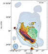 |
Fig. 1. Composite MUSE–MeerKAT image of the jellyfish galaxy JO147. We show the stellar disk (dashed black contour), the Hα emission (orange to black color map), the radio continuum emission at 1.4 GHz (blue-scale contours, from a signal-to-noise of three up to 600, angular resolution 12 × 12 arcsec2, noise level of 7 μJy beam−1), and the polarized emission with a signal-to-noise ratio higher than five (green contours). The intensity of the green contours and the length of the magnetic field vectors (black lines) are proportional to the polarization fraction. The physical scale is shown in the top-right corner, whereas the blue and red circles in the left corner respectively show the radio continuum and Hα image resolution. |
3. Magnetic field orientations
3.1. New evidence of extraplanar polarized emission in JO147
In JO147, MeerKAT detected a 60 kpc long radio continuum tail at 1.4 GHz (Fig. 1), which is consistent with previous findings (Merluzzi et al. 2024), and, for the first time, MeerKAT revealed the presence of polarized synchrotron emission in the tail of this galaxy. The polarized emission in JO147 is present only in the western side of the tail, and it only marginally overlaps with the stripped warm ISM, traced by the Hα emission (Poggianti et al. 2019a). The total polarized flux density is 0.13 mJy, with an average polarized emission fraction of 10%. We further observed that the polarization fraction is higher in the region where it does not overlap with the Hα emission. The polarized angle vector analysis showed that the magnetic field is mainly oriented parallel to the stellar disk. The polarized signal associated with JO147 is characterized by a Faraday rotation measure pattern (Fig. 2) ranging between –45 and –20 rad m−2, with a median value of –30 rad m−2, and a tentative gradient along the stripping tail. The Galactic foreground in this region contributes only ∼4 rad m−2 according to Hutschenreuter et al. (2022), implying that the signal is either generated by the ICM in front of the galaxy or is intrinsic to the source.
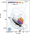 |
Fig. 2. Composite MUSE–MeerKAT image of the jellyfish galaxy JO147. All quantities are identical to those shown in Fig. 1, but the color-filled contours now represent the Faraday rotation measure map. |
3.2. Differences in magnetic field configurations between JO206 and JO147
The newly detected polarized emission in JO147 differs from that previously studied in JO206 (Müller et al. 2021), specifically in terms of extension, magnetic field geometry, and Faraday rotation measure signal. We observed that the polarized emission in JO147 is limited to the tail, whereas in JO206 it extends from the stellar disk down to the stripped tail. Common to both galaxies is an increasing polarization fraction from the disk to the tail. Concerning the magnetic field direction, we observed a striking difference where the field appears to be parallel to the stellar disk in JO147 and perpendicular to it in JO206. Furthermore, the two galaxies show a difference in rotation measure. In JO206, Müller et al. (2021) reported, after correcting for the Galactic foreground (∼5.8 rad m−2), rotation measure values between –50 and 50 rad m−2, which increase up to 200 rad m−2 toward the tail.
The difference in rotation measure may indicate that the two galaxies reside in different regions of their respective clusters, with JO147 being more peripherical than JO206. This result is in line with the projected clustercentric distance of the two galaxies, which are 0.28 and 0.45 R200 for JO206 and JO147, respectively (Gullieuszik et al. 2020). Additionally, the two galaxies show different inclinations with the ICM wind, with JO147 being mostly face-on stripping and JO206 presenting an edge-on configuration. Preliminary numerical simulations of realistic ICM-winds derived from galaxy orbits in a cosmological zoom-in cluster simulation (Dusch 2025) suggest that the fraction and orientation of the polarized emission in the tail can change with time during the galaxy infall in the cluster, becoming increasingly aligned with the stripped material as the galaxy plunges into the cluster. These preliminary results suggest the existence of an evolutionary sequence that can explain the critical difference between the magnetic field configurations in the two galaxies. Additional work in this direction is therefore needed to fully explore how disk inclination and the presence of a galactic wind, gaseous environment, and orbit phase affect the magnetic field orientation of the ordered component along the galaxy and its tail. In this work we present a potential framework to interpret the differences in the magnetic field configuration and the extraplanar star formation between JO147 and JO206.
4. Supersonic-driven versus ram pressure-driven star formation
4.1. The role of supersonic motions
As outlined in Sect. 1, the extraplanar magnetic field can be composed of two components, an internal one deriving from the stripped ISM magnetic field and an external one provided by the ICM draping. The resulting polarized emission should therefore depend on the balance between the intensity of these two components. In the following, we present a physical framework to link the observed differences between JO147 and JO206 to a potential different balance between stripped and draped magnetic field intensities. To begin with, the paucity of coherent polarized emission in JO147, especially in the disk, suggests that the galaxy’s magnetic field is mixed with the thermal plasma, which depolarizes most of the nonthermal emission via Faraday rotation. So we detect polarized emission mostly in the regions where the warm ISM and the corresponding Hα emission are less present. In contrast, in JO206 the polarized emission was detected from the stellar disk up to the stripped tail. Furthermore, the polarization angle suggests that the magnetic field is mostly aligned with the disk in JO147 instead of the stripped tail. We argue that this is because we are either observing (1) the ISM magnetic field being stripped from the stellar disk; (2) a different upstream magnetic field orientation that is illuminated by cosmic ray electrons in the magnetic drape (Pfrommer & Dursi 2010), in which case the opposite polarization vectors orientation in JO206 would probe a different upstream orientation of the ICM magnetic field; or (3) an early phase of the magnetic drape formation, with a recent passing of the cluster accretion shock.
The galaxy JO147 has a projected velocity along the line of sight of 664 km s−1 (Gullieuszik et al. 2020), which is greater than the typical ICM Alfvén speed, and so it would be in the condition to form a magnetic drape. Hence, we argue that the lack of abundant coherent continuum emission from it can be due to one of two factors: either a scarcity of cosmic ray electrons coming from the stellar disk to light up the magnetic drape or a low drape magnetic field energy density, hence low synchrotron emissivity. Both JO147 and JO206 are currently forming stars in their disk (Vulcani et al. 2018; Gullieuszik et al. 2020) and show extended radio continuum tails, which indicates that in both systems there are cosmic rays available to illuminate the drape, hence challenging the first possibility. On the other hand, the drape magnetic energy density, ϵB, depends on the galaxy velocity (Dursi & Pfrommer 2008), and it can be expressed as ϵB = αγℳ2PICM, where α ≃ 2 is the geometrical factor (Dursi & Pfrommer 2008); ℳ = V/cs is the Mach number, where V is the galaxy velocity and cs is the local sound speed; γ is the ICM adiabatic index; and PICM is the ICM thermal pressure. If the galaxy has reached a sufficient velocity to become supersonic, i.e., ℳ = V/cs > 1, then the shock compression can further amplify the field strength (Sparre et al. 2020). Therefore, we argue that the key factor that differentiates the two galaxies and leads to different properties in their tail is that JO147 experienced a weaker shock compression than JO206 resulting from a low-Mach motion in the ICM. As a direct consequence, JO147 has not formed a strong magnetic drape yet, which resulted in an extraplanar magnetic field dominated by the stripped ISM (hence limited polarized emission) and fast evaporation of the stripped material due to the lack of a protective magnetic drape. Supersonic motions can also have another implication. The resulting counter shock crossing the galaxy can impose a compression on the ISM, which depends on the shock Mach number. The compression increases the ISM density, which results in more efficient cooling. In the case of significant ISM compression, the dense stripped clouds efficiently cool down and thus become resilient to thermal evaporation (Gronke & Oh 2018). In this framework, a weak shock compression in JO147 would have resulted in both stripped ISM clouds being less resilient to the external heating, due to the lower density, and a weak magnetic drape that could not shield the stripped gas from the ICM.
To test this hypothesis, it is necessary to constrain the JO147 3D galaxy velocity with respect to the ICM and the corresponding Mach number. The velocity component along the line of sight can be derived from the spectroscopic optical observation of the galaxy, whereas the perpendicular component, which is consistent with the stripped ISM velocity along the plane of the sky (Roberts et al. 2024a), can be constrained from the curvature of the radio continuum gradient along the stripped tail by following the approach described in Ignesti et al. (2023). The radio emission was sampled using the PT-REX code3 (Ignesti 2022) with a hexagonal grid, where each bin is as large as the resolution of the radio continuum image, 12 × 12 arcsec2. The grid covers the radio emission outside of the stellar disk and with a signal-to-noise ratio higher than three. To compose the radio flux density profile, for each bin we measured the radio continuum flux density and the projected distance from the stellar disk, which we measured as the shortest path from the center of the cell to the stellar disk mask edge. The profile was then fit with the semi-empirical model derived under the assumption that (1) the relativistic electrons are accelerated only in the stellar disk, and they leave it on a timescale significantly shorter than the energy loss timescale; (2) the energy losses outside of the stellar disk are dominated by synchrotron and Inverse Compton radiation; (3) the relativistic electrons bulk motion is described by a uniform velocity along the stripping direction; and (4) the electrons move in a uniform magnetic field (Ignesti et al. 2023). The model is fitted to the observed profile by using the least squares method to derive the best-fitting velocity and amplitude in flux density units, as well as the associate uncertainties.
We observed that the radio continuum flux density profile along the tail (Fig. 3) shows a monotonic decline with distance. When adopting a typical range for magnetic field intensity, B = 2 − 5 μG, along the stripped tails (Ignesti et al. 2022; Roberts et al. 2024a), the best-fitting profile returns an average velocity along the plane of the sky in the range V⊥ = 762 − 1089 km s−1. Adding V⊥ in quadrature with the velocity component along the line of sight, V∥ = 664 km s−1 (Gullieuszik et al. 2020), derived from the MUSE spectroscopical observations, results in a total velocity of  km s−1. Previous studies (Bardelli et al. 1996) of the ICM thermal properties at the galaxy clustercentric distance (13.8 arcmin, corresponding to ∼876 kpc at the cluster redshift) permit us to constrain the local sound speed at cs ≃ 800 km s−1, resulting in a Mach number in the range ℳ = 1.3 − 1.6, which entails a weak compression in accordance with our hypothesis.
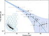 |
Fig. 3. Radio flux density vs. distance from the stellar disk edge. In the left corner, we show the sampling grid overlayed on the radio continuum emission shown in Fig. 1. The best-fitting profile is shown by the blue line. The blue-shaded region indicates the 1σ uncertainties on the fit. |
We note that, as discussed in Ignesti et al. (2023), a crucial caveat of this method is the nonlinear magnetic field intensity-velocity degeneracy due to the fact that a strong (weak) magnetic field entails short (long) cooling timescales, and hence a high (low) velocity is required for the radio plasma to extend over the observed radio tail length. For reference, JO147 would achieve ℳ > 2 only for B > 7 μG, which would be larger than typically inferred for this class of galaxies (Müller et al. 2021; Ignesti et al. 2022; Roberts et al. 2024a). We further note that a direct comparison with JO206 is not possible because Müller et al. (2021) could only derive a lower limit, ℳ > 1.3, under the assumption that the velocity component along the line of sight was equal to the perpendicular component. However, the galaxy morphology suggests that the perpendicular component is significantly larger than the parallel one (Jaffé et al. 2018). Moreover, the radio emission gradient analysis cannot be performed on JO206 because, due to the high extraplanar star formation, the assumption of relativistic electrons originating only in the disk is not respected.
4.2. Testing the general implications
In our proposed framework, the star-forming tails of jellyfish galaxies result from the shock compression they experience during their orbits. It would then follow that galaxies with a higher Mach number should exhibit a relatively higher amount of star formation in their tails. To test this prediction, we examined a sample of jellyfish galaxies from the GASP sample (Gas Stripping Phenomena in Galaxies with MUSE, Poggianti et al. 2017, 2025) to compare their capability in forming stars outside of their stellar disk with their Mach number. In principle, an accurate measure of a cluster galaxy Mach number would require high-angular resolution X-ray observations to determine the morphology and the spectral properties of the bow shock induced in the ICM (e.g., Weżgowiec et al. 2011; Poggianti et al. 2019b), in which temperature and density jumps between upstream and downstream are directly related to the shock Mach number. However, this measurement is often contaminated by projection effects, which can smooth out the thin temperature and density jump induced by the galaxies or the generally low surface brightness, which makes determining the spectral properties of the up- and downstream regions difficult. Therefore, in this work we propose analyzing the “statistical” Mach number.
As a reference, we first computed the “projected” Mach number, which we calculated as the line-of-sight velocity component divided by the average ICM sound speed, which is based on the average ICM temperature. The star formation rate of GASP galaxies as well as the amount of star formation taking place outside of the stellar disks have been calculated from MUSE observations previously (Gullieuszik et al. 2020). Their relative amount of extraplanar star formation was estimated from both the fraction of star formation in the tail, Ftail, which comes from the ratio between the extraplanar and the total star formation, and the extraplanar specific star formation rate, sSFRtail, derived by dividing the extraplanar star formation rates by the corresponding total stellar mass, M*, which correlates with the total star formation (Vulcani et al. 2018). The final sample we used is composed of 17 spiral galaxies in a state of strong or extreme stripping (Morphological type T > −1 and Jtype = 1,2, see Vulcani et al. 2015; Poggianti et al. 2025), with Ftail > 0.01, to ensure a minimum amount of extraplanar star formation, and a projected cluster-centric distance lower than R500, the physical radius within which the average cluster density exceeds 500 times the critical universe density at that redshift.
In the projected analysis, shown in Fig. 4, a positive trend between the “projected” Mach number and the extraplanar star formation efficiency emerged, which is in line with our hypothesis. However, the projected Mach number is a lower limit of its real value. In order to further test the trends shown in Fig. 4, we used a statistical method to infer the 3D velocity and cluster-centric distance of GASP jellyfishes by matching their location in phase-space with those produced by a realistic family of orbits integrated within the cluster gravitational potential.
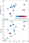 |
Fig. 4. Extraplanar star formation efficiency vs. “projected” Mach number. Extraplanar specific star formation rate, log10(sSFRtail) (top), and star formation rate fraction, log10(Ftail) (bottom), vs. projected Mach number lower limits, ℳ. Each galaxy is color coded according to its total star formation rate (Gullieuszik et al. 2020). JO147 and JO206 are marked with red and blue circles, respectively. |
For each galaxy, we simulated the possible 3D orbits within the hosting cluster to derive the distributions of their 3D velocity and position in order to associate them with their projected counterparts. The hosting cluster gravitational potential was modeled as an NFW profile (Navarro et al. 1997), where the mass and concentration parameters, namely, M200 and c, were previously derived in Biviano et al. (2017). The integration of each orbit was carried out with the gala Python package (Price-Whelan 2017). Every orbit started from a random point on a sphere with a radius equal to R200 from the cluster center and with the infall velocities randomly sampled from the distributions of tangential and radial velocities, rescaled for the hosting cluster velocity dispersion, presented in Smith et al. (2022). These distributions were derived from the orbits of dark matter halos on their first infall into a sample of nearly 740 groups and clusters in cosmological simulations. For each of the 42353 infalling galaxies, the tangential and radial component of their velocity was measured at the moment of crossing R200 of the group or cluster. To replicate the typical radial orbits of jellyfish galaxies (Wetzel & White 2010; Rhee et al. 2017; Biviano et al. 2024), only orbits with a ratio between the initial radial and tangential components larger than 1.4 were selected. Relaxing this assumption generally results in lower Mach number estimates, but it does not change the trends. Observational evidence suggests that optically selected jellyfish galaxies preferentially form their tail during their first infall (Smith et al. 2022; Salinas et al. 2024). Accordingly, each orbit was simulated until it reached the pericenter and was then projected into phase-space coordinates by considering the distance along the x-axis as the projected cluster-centric distance and the velocity along the y-axis as the line-of-sight velocity. When a projected orbit crosses the observed phase-space coordinates, within an interval of 10% of their observed values, the corresponding values of 3D velocity and distance are stored.
To compute the Mach number corresponding to a given pair of 3D velocity-distance coordinates, it is necessary to know the local ICM sound speed, which, under the assumption of monoatomic thermal gas, depends only on the ICM temperature as  km s−1. The ICM temperature profile was modeled using the averaged analytical profile presented in Vikhlinin et al. (2006). The average ICM temperature of each cluster was estimated as the median of the values reported in previous X-ray studies (David et al. 1993; Cavagnolo et al. 2009; Sanderson et al. 2006; Poggianti et al. 2019b; Müller et al. 2021; Bartolini et al. 2022; Bulbul et al. 2024). For each orbit, the temperature profile was assumed to vary within a 15% scatter resulting from the analytical profile uncertainty. The analytical temperature profile was considered valid only within R500, which represents an additional condition to select the 3D velocity-distance pairs. The corresponding 3D Mach number for each orbit was ultimately computed as ℳi = Vi/cs(Ri), where the i subscript indicates the iteration. We repeated the simulation until we collected a distribution of 1000 Mach values per galaxy or when we had run 105 orbits. The final Mach number estimates, and their uncertainties, were computed from the median and the 16th and 84th percentiles of the distribution. The ram pressure (Pram) was computed by modeling the ICM density profile following Pratt et al. (2022), including the scatter on the best-fitting parameters. Similar to the case of the Mach number, we derived a distribution of Pram composed of each 3D velocity-distance combination consistent with their projected counterparts as Pram, i = ρ(Ri)Vi2. Then the final estimates and their uncertainties were computed from the median and the 16th and 84th percentiles of the distributions. In Table 1, we report the input parameter for each galaxy, the resulting estimates of ℳ3D and Pram, and the percentage of success (Sp), computed as the ratio between the number of orbits crossing the phase-space coordinates and the total number of simulated orbits. As an example, we show the Monte Carlo analysis steps for the galaxy JO147 in Fig. 5. Specifically, we show the projected simulated orbits in comparison to the galaxy phase-space coordinates (top-left panel), the distributions of 3D velocities (Vi) and cluster-centric distances (Ri) associated with the projected coordinates (top-right panel), and the resulting ℳi and Pram, i distributions (bottom panels).
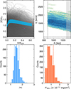 |
Fig. 5. Outcomes of the Monte Carlo analysis for JO147. Top: Simulated orbits projected on the phase-space plane. The red dot shows the projected phase-space coordinates for JO147, and the blue line indicates the corresponding ICM sound speed profile (left) and 2D Distribution of the Vi–Ri pairs associated with the projected JO147 coordinates. The dashed lines indicate the projected coordinates of JO147, and the shaded area covers the rejected Vi–Ri solutions (right). Bottom: ℳi (left) and Pram, i (right) distributions. The vertical lines indicate the median and the 16th and 84th percentiles. |
Galaxy sample parameters.
For GASP jellyfish galaxies, we inferred 1 < ℳ3D < 2.6, which would result in a maximum compression factor of ∼1.9, and  , which are consistent with previous estimates (Weżgowiec et al. 2011; Yun et al. 2019; Ignesti et al. 2023). As an additional sanity check, in Fig. 6 we show that the values of the Mach number and ram pressure inferred with the Monte Carlo analysis for each galaxy follow the expected nonlinear relation
 (1)
(1)
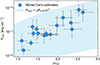 |
Fig. 6. Values of ℳ3D and Pram inferred with the Monte Carlo analysis compared with the expected trend for typical ICM thermal properties (Eq. 1). |
where γ = 5/3 is the adiabatic index and PICM is the ICM thermal pressure computed for the typical ICM particle density between 10−4 and 10−3 cm−3 and temperature between 107 and 108 K. For JO147, the Monte Carlo estimate ℳ3D = 1.5 ± 0.2 is consistent with the measurement based on the radio continuum gradient, ℳ = 1.3 − 1.6. Regarding JO206, we inferred ℳ3D = 1.1 ± 0.1. However, we note that it is one of the cases where the ℳ3D value may be systematically underestimated (for a detailed discussion we refer to Sect. 4.3). In general, with the Monte-Carlo approach, we inferred values of ℳ3D that are systematically higher than the corresponding projected values, with the difference being larger for galaxies showing the lowest line-of-sight velocity.
In Fig. 7 the sSFRtail (top) and Ftail (bottom) are compared with ℳ3D (left) and Pram (right) to determine which factor, shock compression or ram pressure, plays a more significant role in triggering extraplanar star formation. For reference, galaxies are color coded for their total star formation rate. We further quantified the correlation strength by computing the distribution of the Spearman rank ρs from 10 000 random realizations of our dataset, each built by extracting the relevant quantities, ℳ3D and Pram, from normal distributions and with the mean and standard deviations given by each estimate and associated uncertainties. The resulting ρs distribution, shown in Fig. 8, supports a stronger correlation of Ftail and sSFRtail with ℳ3D than with Pram. We found ρs > 0.5 for 51% of the realizations using ℳ3D (Fig. 8, bottom panel), with an average correlation rank of ρs = 0.5 ± 0.1, and ρs > 0.5 was found only for 13% of the realizations using Pram, which instead resulted in an average ρs = 0.2 ± 0.2.
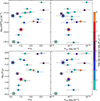 |
Fig. 7. Extraplanar star formation efficiency vs. dynamical properties of the GASP sample. Extraplanar specific star formation rate, log10(sSFRtail) (top), and star formation rate fraction, log10(Ftail) (bottom), vs. 3D Mach number, ℳ3D (left), and ram pressure, Pram (right, presented on a logarithmic scale for visual clarity). Each point is color coded based on its corresponding total star formation rate (Gullieuszik et al. 2020). JO147 and JO206 are marked with red and blue circles, respectively. Points marked with silver boxes may suffer from systematic ℳ3D underestimates (see Sect. 4.3). |
4.3. Caveats
The Monte Carlo analysis presented in this work is subject to a number of caveats and limitations to be taken into consideration. We discuss them in the following list.
-
We observed that the constraint Ri ≤ R500 sets a systematic limit for the Vi and Ri distributions, and correspondingly, it narrows the resulting ℳi distribution.
-
For reference, we also computed the Mach number in the case of an isothermal ICM, corresponding to a case where the sound speed is uniform in the cluster. This model overestimates the sound speed at large distances, hence resulting in generally lower Mach number values than the analytical profile case.
-
We note that this approach assumes spherical symmetry, cluster dynamical equilibrium, and normalization of the infalling velocity to the cluster velocity dispersion. These assumptions may not be a solid representation of systems undergoing mergers, for which the actual temperature is higher than the equilibrium one, or for extremely fast infalling galaxies. In these cases, the Mach number can be underestimated. This effect may explain the low values of ℳ3D we inferred for some of the high star-forming galaxies, signaled with silver boxes in Fig. 7, which are hosted in clusters for which the observed temperature is higher than the one predicted by the mass-temperature scaling relation (Babyk & McNamara 2023). The case of JO206 appears to be especially critical, as it would be a fast infaller in a relatively low mass cluster (M200 ≃ 2 × 10¹⁴ M⊙; Gullieuszik et al. 2020) with, in contrast, a relatively high average ICM temperature of 3.9 keV, which is ∼1.4 times higher than expected given its mass. As a result, our model predicts relatively low velocities with respect to the local ICM sound speed, thus resulting in a low Mach number estimate. Correspondingly, in the so-called cool-core systems, the central temperature can be lower than the one predicted by the analytical model, resulting in an overestimation of the Mach numbers for the orbits crossing the cluster center.
-
With this approach, by construction, Pram and ℳ3D can be inferred with a markedly different precision. Within the inner regions of galaxy clusters, the analytical ICM density profile is significantly steeper than the temperature profile. Consequently, the uncertainty in the determination of the 3D distance produces a larger scatter in Pram than in ℳ3D. Additionally, uncertainties on Pram depend on the square of the uncertainty on the velocity, while it is linear for the Mach number. These effects lead to having larger uncertainties for Pram than for ℳ3D, which is expected to have an impact on simple correlation tests. However, we stress that the analysis shown in Fig. 8, based on the full exploration of the Spearman rank distribution, is meant to bypass these problematics.
-
There are a series of parameters not taken into account in this method, such as disk-wind angle, ISM and ICM substructure, stripping evolutionary stage, ICM and ISM magnetic field orientation, and orbital interaction history. Exploring their impact requires tailored MHD simulations.
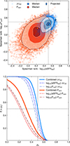 |
Fig. 8. Spearman rank distributions. Top: Spearman rank distributions derived for log10(sSFRtail) and log10(Ftail) when compared with ℳ3D (blue) and Pram (red). Each point shows the ranks derived for different realizations of the ℳ3D and Pram series. The contours indicate the 2D probability density levels of 0.16, 0.5, and 0.84. The dashed black lines indicate the ρs = +0.5, corresponding to an existing positive correlation between the two quantities. The black-outlined points indicate the Spearman ranks measured from the median values reported in Fig. 7. For reference, the blue diamond indicates the correlation rank from the “projected” ℳ (Fig. 4); Bottom: Fraction of realizations with a Spearman rank higher than ρs for ℳ3D (blue) and Pram (red). The solid lines show the combined fractions of log10(sSFRtail) and log10(Ftail), and the dashed and dot-dashed lines show the fractions for the individual quantities. The dashed black lines indicate the 0.5 levels on the corresponding axis. |
5. Conclusions
We have presented an investigation of the extraplanar magnetic field configuration in the galaxy JO147 based on new MeerKAT data, and we find it differs substantially from the only other known case, JO206. We argue that this is because the two galaxies experienced different supersonic compressions during their orbit, resulting in different magnetic drape intensities, and in the case of JO206, the stronger compression enabled extraplanar star formation. We then tested this scenario by comparing the Mach number and the extraplanar star formation of 17 GASP galaxies, finding evidence of a moderate positive correlation between these quantities.
Therefore, we propose that the critical factor in forming a jellyfish galaxy could be the compression resulting from its supersonic orbits, which sets the conditions for the stripped ISM and the magnetic field to harbor star formation outside the stellar disk. Our Monte Carlo analysis suggests that the supersonic motion could be more impactful than the ram pressure, but we also note that disentangling the two effects is not trivial because they are both intrinsically dependent on the galaxy velocity. Furthermore, strong ram pressure events could have facilitated the removal of large gas clouds from the galaxy in the early stages of the stripping (Vollmer et al. 2012), which, due to the larger volume-to-surface ratio, would be more resilient to thermal evaporation than smaller ones (Armillotta et al. 2017; Gronke & Oh 2018). Following our proposed framework, JO147 would exemplify a low-Mach-number stripping outcome, where the magnetic field configuration suggests a limited drape influence, and therefore the extraplanar star formation has been limited.
The connection between magnetic field, orbit velocity, and star formation that we have presented in this work can be further explored via numerical simulations, as already pioneered by Sparre et al. (2020, 2024b). Specifically, it would be of foremost interest to use such techniques to address the role of the inclination angle between the stellar disk and the wind as well as the interplay between magnetic drape, star formation feedback, and ICM turbulent mixing (Franchetto et al. 2021; Sun et al. 2021; Ignesti et al. 2024). Furthermore, future wide-field high-angular resolution X-ray observations with the AXIS telescope (Koss et al. 2025) may help confirm this scenario by providing direct Mach number measurements of cluster galaxies by detecting the bow shock induced by their supersonic motions. To further explore this scenario, mapping the magnetic field of large cluster galaxy samples is crucial in order to estimate the incidence of ordered large-scale field configurations via radio continuum observations. A complementary prediction of the proposed framework is that super-sonic galaxies, due to the higher magnetic field intensity in the magnetic drape and subsequent higher synchrotron emissivity, should show a larger fraction of polarized extraplanar emission associated with the ordered magnetic field than other cluster galaxies. However, extraplanar polarized emission is especially elusive in observations because of the combination of two competing processes: the spectral contraction of the radio continuum tails, whose extension typically decrease when they are observed at frequencies above 1 GHz (Ignesti et al. 2022; Roberts et al. 2024b), and the ICM Faraday rotation, which damps the galaxies’ low-frequency polarized signal due to the high ICM density. These combined physical effects, on top of the typical low surface brightness of these sources, makes it difficult to find suitable candidates for these studies. Therefore, we expect that only high-resolution polarimetry surveys between 1 and 2 GHz, such as the MeerKAT Fornax survey (Loi et al. 2025) and, in the future, with the Square Kilometer Array (Loi et al. 2019) in SKA-MID Band 2 can provide us with magnetic field topology for a large sample of cluster galaxies to further explore the physics regulating the evolution of the ISM under extreme conditions set by the ICM ram pressure.
Acknowledgments
We acknowledge the constructive contribute of the Reviewers that improved the presentation of our work. AI thanks A. Biviano for the useful discussion. We are grateful to the full MeerKAT team for their work building, commissioning and operating MeerKAT, and for their support to the MeerKAT Fornax Survey. The MeerKAT telescope is operated by the South African Radio Astronomy Observatory, which is a facility of the National Research Foundation, an agency of the Department of Science and Innovation. Based on observations collected at the European Organization for Astronomical Research in the Southern Hemisphere under ESO programme 196.B-0578. This project has received funding from the European Research Council (ERC) under the European Union’s Horizon 2020 research and innovation programme (grant agreement No. 833824). CP acknowledges support by the European Research Council under ERC-AdG grant PICOGAL-101019746. YLJ acknowledges support from the Agencia Nacional de Investigación y Desarrollo (ANID) through Basal project FB210003, FONDECYT Regular projects 1241426 and 123044, and Millennium Science Initiative Program NCN2024_112. GP acknowledges funding from the European Union – NextGenerationEU, RRF M4C2 1.1, Project 2022JZJBHM: “AGN-sCAN: zooming-in on the AGN-galaxy connection since the cosmic noon” – CUP C53D23001120006. PK is partially supported by the BMBF project 05A23PC1 for D-MeerKAT III. (Part of) the data published here have been reduced using the CARACal pipeline, partially supported by ERC Starting grant number 679627 “FORNAX”, MAECI Grant Number ZA18GR02, DST-NRF Grant Number 113121 as part of the ISARP Joint Research Scheme, and BMBF project 05A17PC2 for D-MeerKAT. Information about CARACal can be obtained online under the URL: https://caracal.readthedocs.io. A.E.L. and B.V. acknowledge support from the INAF GO grant 2023 “Identifying ram pressure induced unwinding arms in cluster spirals” (P.I. Vulcani). The Enhancement of the SRT for the study of the Universe at high radio frequencies is financially supported by the National Operative Program (Programma Operativo Nazionale – PON) of the Italian Ministry of University and Research “Research and Innovation 2014-2020”, Notice D.D. 424 of 28/02/2018 for the granting of funding aimed at strengthening research infrastructures, in implementation of the Action II.1 – Project Proposal PIR01_00010. This work was carried out thanks to the funding of the Regione Autonoma della Sardegna, ai sensi della Legge Regionale 7 agosto 2007, n.7 “Promozione della Ricerca Scientifica e dell’Innovazione Tecnologica in Sardegna”. AI thanks the music of Foxy Shazam for inspiring the preparation of the draft.
References
- Armillotta, L., Fraternali, F., Werk, J. K., Prochaska, J. X., & Marinacci, F. 2017, MNRAS, 470, 114 [NASA ADS] [CrossRef] [Google Scholar]
- Babyk, I. V., & McNamara, B. R. 2023, ApJ, 946, 54 [NASA ADS] [CrossRef] [Google Scholar]
- Bardelli, S., Zucca, E., Malizia, A., et al. 1996, A&A, 305, 435 [NASA ADS] [Google Scholar]
- Bartolini, C., Ignesti, A., Gitti, M., et al. 2022, ApJ, 936, 74 [NASA ADS] [CrossRef] [Google Scholar]
- Biviano, A., Moretti, A., Paccagnella, A., et al. 2017, A&A, 607, A81 [NASA ADS] [CrossRef] [EDP Sciences] [Google Scholar]
- Biviano, A., Poggianti, B. M., Jaffé, Y., et al. 2024, ApJ, 965, 117 [Google Scholar]
- Boselli, A., Fossati, M., & Sun, M. 2022, A&ARv, 30, 3 [NASA ADS] [CrossRef] [Google Scholar]
- Bulbul, E., Liu, A., Kluge, M., et al. 2024, A&A, 685, A106 [NASA ADS] [CrossRef] [EDP Sciences] [Google Scholar]
- Cavagnolo, K. W., Donahue, M., Voit, G. M., & Sun, M. 2009, ApJS, 182, 12 [Google Scholar]
- David, L. P., Slyz, A., Jones, C., et al. 1993, ApJ, 412, 479 [Google Scholar]
- Di Gennaro, G., Venturi, T., Giacintucci, S., et al. 2025, A&A, 694, A28 [NASA ADS] [CrossRef] [EDP Sciences] [Google Scholar]
- Dursi, L. J., & Pfrommer, C. 2008, ApJ, 677, 993 [NASA ADS] [CrossRef] [Google Scholar]
- Dusch, N. 2025, Master Thesis, Universität Potsdam [Google Scholar]
- Ebeling, H., Stephenson, L. N., & Edge, A. C. 2014, ApJ, 781, L40 [Google Scholar]
- Franchetto, A., Tonnesen, S., Poggianti, B. M., et al. 2021, ApJ, 922, L6 [NASA ADS] [CrossRef] [Google Scholar]
- Frank, A., Jones, T. W., Ryu, D., & Gaalaas, J. B. 1996, ApJ, 460, 777 [Google Scholar]
- George, S. J., Stil, J. M., & Keller, B. W. 2012, PASA, 29, 214 [Google Scholar]
- George, K., Poggianti, B. M., Vulcani, B., et al. 2025, A&A, 700, A38 [NASA ADS] [CrossRef] [EDP Sciences] [Google Scholar]
- Girardi, M., Biviano, A., Giuricin, G., Mardirossian, F., & Mezzetti, M. 1993, ApJ, 404, 38 [NASA ADS] [CrossRef] [Google Scholar]
- Govoni, F., & Feretti, L. 2004, Int. J. Mod. Phys. D, 13, 1549 [Google Scholar]
- Gronke, M., & Oh, S. P. 2018, MNRAS, 480, L111 [Google Scholar]
- Gullieuszik, M., Poggianti, B. M., McGee, S. L., et al. 2020, ApJ, 899, 13 [Google Scholar]
- Gunn, J. E., & Gott, J. R. 1972, ApJ, 176, 1 [NASA ADS] [CrossRef] [Google Scholar]
- Hester, J. A. 2006, ApJ, 647, 910 [Google Scholar]
- Hutschenreuter, S., Anderson, C. S., Betti, S., et al. 2022, A&A, 657, A43 [NASA ADS] [CrossRef] [EDP Sciences] [Google Scholar]
- Ignesti, A. 2022, New Astron., 92, 101732 [NASA ADS] [CrossRef] [Google Scholar]
- Ignesti, A., Vulcani, B., Poggianti, B. M., et al. 2022, ApJ, 924, 64 [NASA ADS] [CrossRef] [Google Scholar]
- Ignesti, A., Vulcani, B., Botteon, A., et al. 2023, A&A, 675, A118 [NASA ADS] [CrossRef] [EDP Sciences] [Google Scholar]
- Ignesti, A., Brunetti, G., Gullieuszik, M., et al. 2024, ApJ, 977, 219 [Google Scholar]
- Jaffé, Y. L., Poggianti, B. M., Moretti, A., et al. 2018, MNRAS, 476, 4753 [Google Scholar]
- Jonas, J., & MeerKAT, T. 2016, MeerKAT Science: On the Pathway to the SKA, 1 [Google Scholar]
- Józsa, G. I. G., White, S. V., Thorat, K., et al. 2020, ASP Conf. Ser., 527, 635 [Google Scholar]
- Klein, R. I., McKee, C. F., & Colella, P. 1994, ApJ, 420, 213 [Google Scholar]
- Koss, M., Aftab, N., Allen, S. W., et al. 2025, arXiv e-prints [arXiv:2511.00253] [Google Scholar]
- Lee, J., Kimm, T., Blaizot, J., et al. 2022, ApJ, 928, 144 [NASA ADS] [CrossRef] [Google Scholar]
- Li, Z., Hopkins, P. F., Squire, J., & Hummels, C. 2020, MNRAS, 492, 1841 [NASA ADS] [CrossRef] [Google Scholar]
- Li, Y., Luo, R., Fossati, M., Sun, M., & Jáchym, P. 2023, MNRAS, 521, 4785 [NASA ADS] [CrossRef] [Google Scholar]
- Loi, F., Murgia, M., Govoni, F., et al. 2019, MNRAS, 485, 5285 [NASA ADS] [CrossRef] [Google Scholar]
- Loi, F., Serra, P., Murgia, M., et al. 2025, A&A, 694, A125 [NASA ADS] [CrossRef] [EDP Sciences] [Google Scholar]
- McCourt, M., O’Leary, R. M., Madigan, A.-M., & Quataert, E. 2015, MNRAS, 449, 2 [NASA ADS] [CrossRef] [Google Scholar]
- Merluzzi, P., Busarello, G., Haines, C. P., et al. 2015, MNRAS, 446, 803 [NASA ADS] [CrossRef] [Google Scholar]
- Merluzzi, P., Venturi, T., Busarello, G., et al. 2024, MNRAS, 533, 1394 [Google Scholar]
- Müller, A., Poggianti, B. M., Pfrommer, C., et al. 2021, Nat. Astron., 5, 159 [Google Scholar]
- Navarro, J. F., Frenk, C. S., & White, S. D. M. 1997, ApJ, 490, 493 [Google Scholar]
- Offringa, A. R., van de Gronde, J. J., & Roerdink, J. B. T. M. 2012, A&A, 539, A95 [NASA ADS] [CrossRef] [EDP Sciences] [Google Scholar]
- Perley, R. A., & Butler, B. J. 2017, ApJS, 230, 7 [NASA ADS] [CrossRef] [Google Scholar]
- Pfrommer, C., & Dursi, L. J. 2010, Nat. Phys., 6, 520 [NASA ADS] [CrossRef] [Google Scholar]
- Poggianti, B. M., Fasano, G., Omizzolo, A., et al. 2016, AJ, 151, 78 [Google Scholar]
- Poggianti, B. M., Moretti, A., Gullieuszik, M., et al. 2017, ApJ, 844, 48 [Google Scholar]
- Poggianti, B. M., Gullieuszik, M., Tonnesen, S., et al. 2019a, MNRAS, 482, 4466 [Google Scholar]
- Poggianti, B. M., Ignesti, A., Gitti, M., et al. 2019b, ApJ, 887, 155 [Google Scholar]
- Poggianti, B. M., Vulcani, B., Tomicic, N., et al. 2025, A&A, 699, A357 [NASA ADS] [CrossRef] [EDP Sciences] [Google Scholar]
- Pratt, G. W., Arnaud, M., Maughan, B. J., & Melin, J. B. 2022, A&A, 665, A24 [NASA ADS] [CrossRef] [EDP Sciences] [Google Scholar]
- Price-Whelan, A. M. 2017, J. Open Source Software, 2 [Google Scholar]
- Purcell, C. R., Van Eck, C. L., West, J., Sun, X. H., & Gaensler, B. M. 2020, Astrophysics Source Code Library [record ascl:2005.003] [Google Scholar]
- Rhee, J., Smith, R., Choi, H., et al. 2017, ApJ, 843, 128 [Google Scholar]
- Rintoul, T. A., van de Voort, F., Hannington, A. T., et al. 2025, MNRAS, 543, 4321 [Google Scholar]
- Roberts, I. D., van Weeren, R. J., de Gasperin, F., et al. 2024a, A&A, 689, A22 [NASA ADS] [CrossRef] [EDP Sciences] [Google Scholar]
- Roberts, I. D., van Weeren, R. J., Lal, D. V., et al. 2024b, A&A, 683, A11 [NASA ADS] [CrossRef] [EDP Sciences] [Google Scholar]
- Rohr, E., Pillepich, A., Nelson, D., et al. 2023, MNRAS, 524, 3502 [NASA ADS] [CrossRef] [Google Scholar]
- Rossetti, M., Ghizzardi, S., Molendi, S., & Finoguenov, A. 2007, A&A, 463, 839 [NASA ADS] [CrossRef] [EDP Sciences] [Google Scholar]
- Salinas, V., Jaffé, Y. L., Smith, R., et al. 2024, MNRAS, 533, 341 [NASA ADS] [CrossRef] [Google Scholar]
- Sanderson, A. J. R., Ponman, T. J., & O’Sullivan, E. 2006, MNRAS, 372, 1496 [NASA ADS] [CrossRef] [Google Scholar]
- Sarazin, C. L. 1988, X-ray emission from clusters of galaxies [Google Scholar]
- Serra, P., Westmeier, T., Giese, N., et al. 2015, MNRAS, 448, 1922 [Google Scholar]
- Serra, P., Oosterloo, T. A., Kamphuis, P., et al. 2024, A&A, 690, A4 [NASA ADS] [CrossRef] [EDP Sciences] [Google Scholar]
- Shapley, H. 1930, Harvard College Obs. Bull., 874, 9 [Google Scholar]
- Smith, R. J., Lucey, J. R., Hammer, D., et al. 2010, MNRAS, 408, 1417 [Google Scholar]
- Smith, R., Shinn, J.-H., Tonnesen, S., et al. 2022, ApJ, 934, 86 [NASA ADS] [CrossRef] [Google Scholar]
- Sparre, M., Pfrommer, C., & Vogelsberger, M. 2019, MNRAS, 482, 5401 [Google Scholar]
- Sparre, M., Pfrommer, C., & Ehlert, K. 2020, MNRAS, 499, 4261 [NASA ADS] [CrossRef] [Google Scholar]
- Sparre, M., Pfrommer, C., & Puchwein, E. 2024a, A&A, 691, A259 [NASA ADS] [CrossRef] [EDP Sciences] [Google Scholar]
- Sparre, M., Pfrommer, C., & Puchwein, E. 2024b, MNRAS, 527, 5829 [Google Scholar]
- Spitzer, L. 1978, Physical processes in the interstellar medium [Google Scholar]
- Sun, M., Ge, C., Luo, R., et al. 2021, Nat. Astron., 6, 270 [NASA ADS] [CrossRef] [Google Scholar]
- Sun, M., Le, H., Epinat, B., et al. 2026, A&A, 705, A139 [NASA ADS] [CrossRef] [EDP Sciences] [Google Scholar]
- Venturi, T., Bardelli, S., Morganti, R., & Hunstead, R. W. 2000, MNRAS, 314, 594 [NASA ADS] [CrossRef] [Google Scholar]
- Venturi, T., Giacintucci, S., Merluzzi, P., et al. 2022, A&A, 660, A81 [NASA ADS] [CrossRef] [EDP Sciences] [Google Scholar]
- Vikhlinin, A., Kravtsov, A., Forman, W., et al. 2006, ApJ, 640, 691 [Google Scholar]
- Vollmer, B., Cayatte, V., Balkowski, C., & Duschl, W. J. 2001, ApJ, 561, 708 [NASA ADS] [CrossRef] [Google Scholar]
- Vollmer, B., Thierbach, M., & Wielebinski, R. 2004, A&A, 418, 1 [NASA ADS] [CrossRef] [EDP Sciences] [Google Scholar]
- Vollmer, B., Soida, M., Braine, J., et al. 2012, A&A, 537, A143 [NASA ADS] [CrossRef] [EDP Sciences] [Google Scholar]
- Vollmer, B., Sun, M., Jachym, P., Fossati, M., & Boselli, A. 2024, A&A, 692, A4 [NASA ADS] [CrossRef] [EDP Sciences] [Google Scholar]
- Vulcani, B., Poggianti, B. M., Fritz, J., et al. 2015, ApJ, 798, 52 [Google Scholar]
- Vulcani, B., Poggianti, B. M., Gullieuszik, M., et al. 2018, ApJ, 866, L25 [Google Scholar]
- Waldron, W., Sun, M., Luo, R., et al. 2023, MNRAS, 522, 173 [NASA ADS] [CrossRef] [Google Scholar]
- Westmeier, T., Kitaeff, S., Pallot, D., et al. 2021, MNRAS, 506, 3962 [NASA ADS] [CrossRef] [Google Scholar]
- Wetzel, A. R., & White, M. 2010, MNRAS, 403, 1072 [NASA ADS] [CrossRef] [Google Scholar]
- Weżgowiec, M., Vollmer, B., Ehle, M., et al. 2011, A&A, 531, A44 [NASA ADS] [CrossRef] [EDP Sciences] [Google Scholar]
- Yun, K., Pillepich, A., Zinger, E., et al. 2019, MNRAS, 483, 1042 [Google Scholar]
All Tables
All Figures
|
Fig. 1. Composite MUSE–MeerKAT image of the jellyfish galaxy JO147. We show the stellar disk (dashed black contour), the Hα emission (orange to black color map), the radio continuum emission at 1.4 GHz (blue-scale contours, from a signal-to-noise of three up to 600, angular resolution 12 × 12 arcsec2, noise level of 7 μJy beam−1), and the polarized emission with a signal-to-noise ratio higher than five (green contours). The intensity of the green contours and the length of the magnetic field vectors (black lines) are proportional to the polarization fraction. The physical scale is shown in the top-right corner, whereas the blue and red circles in the left corner respectively show the radio continuum and Hα image resolution. |
| In the text | |
|
Fig. 2. Composite MUSE–MeerKAT image of the jellyfish galaxy JO147. All quantities are identical to those shown in Fig. 1, but the color-filled contours now represent the Faraday rotation measure map. |
| In the text | |
|
Fig. 3. Radio flux density vs. distance from the stellar disk edge. In the left corner, we show the sampling grid overlayed on the radio continuum emission shown in Fig. 1. The best-fitting profile is shown by the blue line. The blue-shaded region indicates the 1σ uncertainties on the fit. |
| In the text | |
|
Fig. 4. Extraplanar star formation efficiency vs. “projected” Mach number. Extraplanar specific star formation rate, log10(sSFRtail) (top), and star formation rate fraction, log10(Ftail) (bottom), vs. projected Mach number lower limits, ℳ. Each galaxy is color coded according to its total star formation rate (Gullieuszik et al. 2020). JO147 and JO206 are marked with red and blue circles, respectively. |
| In the text | |
|
Fig. 5. Outcomes of the Monte Carlo analysis for JO147. Top: Simulated orbits projected on the phase-space plane. The red dot shows the projected phase-space coordinates for JO147, and the blue line indicates the corresponding ICM sound speed profile (left) and 2D Distribution of the Vi–Ri pairs associated with the projected JO147 coordinates. The dashed lines indicate the projected coordinates of JO147, and the shaded area covers the rejected Vi–Ri solutions (right). Bottom: ℳi (left) and Pram, i (right) distributions. The vertical lines indicate the median and the 16th and 84th percentiles. |
| In the text | |
|
Fig. 6. Values of ℳ3D and Pram inferred with the Monte Carlo analysis compared with the expected trend for typical ICM thermal properties (Eq. 1). |
| In the text | |
|
Fig. 7. Extraplanar star formation efficiency vs. dynamical properties of the GASP sample. Extraplanar specific star formation rate, log10(sSFRtail) (top), and star formation rate fraction, log10(Ftail) (bottom), vs. 3D Mach number, ℳ3D (left), and ram pressure, Pram (right, presented on a logarithmic scale for visual clarity). Each point is color coded based on its corresponding total star formation rate (Gullieuszik et al. 2020). JO147 and JO206 are marked with red and blue circles, respectively. Points marked with silver boxes may suffer from systematic ℳ3D underestimates (see Sect. 4.3). |
| In the text | |
|
Fig. 8. Spearman rank distributions. Top: Spearman rank distributions derived for log10(sSFRtail) and log10(Ftail) when compared with ℳ3D (blue) and Pram (red). Each point shows the ranks derived for different realizations of the ℳ3D and Pram series. The contours indicate the 2D probability density levels of 0.16, 0.5, and 0.84. The dashed black lines indicate the ρs = +0.5, corresponding to an existing positive correlation between the two quantities. The black-outlined points indicate the Spearman ranks measured from the median values reported in Fig. 7. For reference, the blue diamond indicates the correlation rank from the “projected” ℳ (Fig. 4); Bottom: Fraction of realizations with a Spearman rank higher than ρs for ℳ3D (blue) and Pram (red). The solid lines show the combined fractions of log10(sSFRtail) and log10(Ftail), and the dashed and dot-dashed lines show the fractions for the individual quantities. The dashed black lines indicate the 0.5 levels on the corresponding axis. |
| In the text | |
Current usage metrics show cumulative count of Article Views (full-text article views including HTML views, PDF and ePub downloads, according to the available data) and Abstracts Views on Vision4Press platform.
Data correspond to usage on the plateform after 2015. The current usage metrics is available 48-96 hours after online publication and is updated daily on week days.
Initial download of the metrics may take a while.