| Issue |
A&A
Volume 708, April 2026
|
|
|---|---|---|
| Article Number | A115 | |
| Number of page(s) | 18 | |
| Section | Stellar atmospheres | |
| DOI | https://doi.org/10.1051/0004-6361/202558636 | |
| Published online | 01 April 2026 | |
Hot subdwarf stars from the Hamburg Quasar Survey
1
Dr. Karl Remeis-Observatory & ECAP, Astronomical Institute, Friedrich-Alexander University Erlangen-Nuremberg,
Sternwartstr. 7,
96049
Bamberg,
Germany
2
Institut für Physik und Astronomie, Universität Potsdam, Haus 28,
Karl-Liebknecht-Str. 24/25,
14476
Potsdam-Golm,
Germany
3
Institut für Astrophysik und Geophysik, Georg-August-Universität Göttingen,
Friedrich-Hund-Platz 1,
37077
Göttingen,
Germany
★ Corresponding author: This email address is being protected from spambots. You need JavaScript enabled to view it.
Received:
18
December
2025
Accepted:
10
February
2026
Abstract
Hot subluminous stars (subdwarf B&O; sdB, sdO) are evolved low mass stars originating from red giants that lost their envelope almost entirely. The multitude of observed phenomena imply that several pathways may form hot subdwarfs, most involving close binary channels. The Hamburg Quasar Survey (HQS) has led to the discovery of many faint blue stars, including hot subdwarf stars. Many of the HQS-sdB stars have been studied in detail, but analyses of the helium-rich sdOB and sdO stars are lacking. The recent development of model spectra calulated from model atmopheres in local thermodynamic equilibrium (LTE) allowing for non-LTE departures (hybrid LTE/NLTE model spectra, the 2nd generation Bamberg model grids) enables us to improve the spectroscopic analyses of sdB stars as well as of the previously unstudied sdO stars allowing precise atmospheric parameters to be derived, while consistently accounting for parameter correlations and systematic uncertainties. The Gaia mission provided astrometric data of unprecedented quality, which allow fundamental stellar parameters to be derived from atmospheric parameters via parallax measurements. We used spectral energy distributions to identify composite-colour sdB binaries and present the result of detailed spectroscopic analyses of 122 non-composite subdwarfs from the HQS to identify potential evolutionary pathways. Comparison to evolutionary tracks both in the Kiel (Teff-log g) and the physical Hertzsprung–Russell (Teff–logL) diagram finds the location of the sdB stars on the extreme horizontal branch (EHB). Their derived mass distribution and median mass of 0.45 M⊙ are consistent with the canonical EHB mass. We revisited the sample of known pulsating HQS-sdB stars and find no significant differences between their mass distributions and those of sdB stars that do not pulsate. The helium-rich sdOB and sdO stars are found near the helium main sequence (He-MS). The derived mass distribution of the extremely He-rich subdwarfs is broader (0.48–1.05 M⊙) and peaks at a median of 0.70 M⊙, significantly larger than those of the hydrogen-rich stars. Intermediate He-rich subdwarfs are also He-MS stars, but of lower mass (0.55 M⊙) than the extremely He-rich subdwarfs. This strongly supports the merger scenario for the origin of He-rich sdO stars, in which two helium white dwarfs merge following orbital decay driven by gravitational-wave emission, producing a He-rich sdO or sdOB star. Comparing results from similar studies, we speculate that older populations produce more massive helium white dwarfs mergers.
Key words: stars: abundances / stars: atmospheres / stars: evolution / Hertzsprung-Russell and C-M diagrams / stars: horizontal-branch / subdwarfs
© The Authors 2026
 Open Access article, published by EDP Sciences, under the terms of the Creative Commons Attribution License (https://creativecommons.org/licenses/by/4.0), which permits unrestricted use, distribution, and reproduction in any medium, provided the original work is properly cited.
This article is published in open access under the Subscribe to Open model. This email address is being protected from spambots. You need JavaScript enabled to view it. to support open access publication.
1 Introduction
Most hot subdwarf stars (subdwarf B&O; sdB, sdO) are low mass stars powered either by helium fusion in the core or by shell burning for the more evolved stars. In the canonical evolutionary scenario, they form the progeny of red giant stars (RGBs) whose hydrogen envelopes have been stripped off near their tip, exposing the helium-burning core following helium ignition (see Heber 2009, 2016, for reviews). The sdB stars are located on the extreme horizontal branch (EHB), exhibiting temperatures ranging from 20 000 to 40 000 K, masses of about half a solar mass, radii from 0.1 to 0.25 solar, and luminosities of about 10−30 solar luminosities. The sdB phase lasts for of the order of a hundred megayears depending mostly on the mass of the sdB (Han et al. 2003). Once helium is exhausted in the core, the stars evolve through the sdO phase, where temperatures exceed 40 000 K and luminosity increases. The mass distribution of these canonical hot subdwarfs is expected to peak at the core mass required for helium ignition under degenerate conditions of 0.45−0.5 M⊙ depending on metallicity. Envelope loss is most easily achieved by mass transfer in close-binary systems via Roche-lobe overflow (RLOF) or common envelope formation and ejection. Thus, it has been suggested that hot subdwarfs reside in close binaries (Mengel et al. 1976), a prediction later confirmed by the detection of many hot subdwarfs in short-period (hours to days) binaries with white dwarf or low mass main-sequence companions (e.g. Maxted et al. 2001). Apparently, single hot subdwarfs can be formed by mergers of two helium white dwarfs driven by gravitational wave emission and magnetic braking and should be located near the helium main sequence in the Hertzsprung-Russell diagram (HRD; Webbink 1984). Their mass distribution is predicted to be much wider than that of canonical subdwarfs (Han et al. 2003) and may produce more massive, helium-rich hot subdwarfs up to about 0.9 M⊙.
Disentangling the various evolutionary pathways requires homogeneous samples of stars with atmospheric parameters derived from quantitative spectral analyses using sophisticated model atmospheres and synthetic spectra. To derive the fundamental stellar parameters, the distances of the stars must be known. Here, parallax measurements by the Gaia mission are crucial, because they allow the atmospheric parameters to be converted to stellar parameters (radius R, luminosity L, and mass M). Homogeneous samples of subdwarfs can be drawn from large surveys such as LAMOST (Luo et al. 2021, 2024) and SDSS (Geier et al. 2024). A brief summary of these developments since the advent of Gaia data releases can be found in Heber (2024). Early photographic surveys for faint blue stars at high Galactic latitudes such as the Palomar-Green (PG; Green et al. 1986), the Byurakan (Lipovetsky et al. 1987; Markarian et al. 1987), the Hamburg objective prism surveys (Hagen et al. 1995; Wisotzki et al. 1996), and their respective spectroscopic follow-up campaigns have been crucial to the field’s development. It is timely to revisit these samples, combining Gaia data with state-of-the-art model atmospheres and analysis techniques. Latour et al. (2026) did so for the PG subdwarf sample. Here we focus on the hot subdwarfs from the Hamburg Quasar Survey (HQS).
The HQS was a photographic wide-angle objective-prism survey to hunt for low-redshift quasars (quasi-stellar objects, QSOs) using the 80 cm Schmidt telescope at the German-Spanish Astronomical Centre (DSAZ) on Calar Alto, Spain (Hagen et al. 1995; Reimers et al. 1996; Hagen et al. 1999). The survey was carried out from 1980 to 1997, with coverage of ≈ 13600 deg2 of the northern sky (δ>0 deg) at high Galactic latitudes (|b| ≳ 20 deg). The magnitude range of the survey is 13 ≲ B ≲ 18.5 mag with spectral coverage from 3400 to 5400 Å and resolution of ∼ 45 Å at Hγ. The plates were scanned and are available through the APPLAUSE database (Enke et al. 2024). Blue objects were classified after visual inspection as candidates for quasars, hot stars, and narrow emission line objects.
Quasars are blue and faint objects, whose population is expected to be outnumbered by evolved stars such as hot white dwarfs, cataclysmic variables, and hot subdwarfs. Quasars can be identified from their strong emission lines, which can be seen in objective prism spectra despite their low resolution (Engels et al. 1988). However, it may be difficult to distinguish QSO objective prism spectra from those of metal-poor halo stars, if their redshift is incompatible with the wavelength coverage of the spectra (Groote et al. 1989). Classification of faint blue stars at such low resolution is difficult (see Homeier & Koester 2001, for details). Hydrogen-rich white dwarfs of intermediate temperatures can be identified through their characteristically broad Balmer absorption lines. For other hot stars, the resolution is too low to resolve spectral features and, therefore, need follow-up spectroscopy to unravel their nature.
Follow-up campaigns of visually selected hot star candidates were carried out at the Calar Alto observatory, mostly using the TWIN Spectrograph at the 3.5 m telescope, resulting in a sample of 400 faint blue stars (Heber et al. 1991). About half turned out to be hot white dwarfs (e.g. Dreizler et al. 1995; Heber et al. 1996; Homeier et al. 1998; Rauch et al. 1998). Others turned out to be cataclysmic variables (more than 50 were found in the HQS survey; Gänsicke et al. 2002; Aungwerojwit et al. 2005; Aungwerojwit & Gänsicke 2009). Our follow-up spectroscopic observations also contributed significantly to the small class of PG 1159 stars (e.g. Dreizler et al. 1994, 1996) and led to the discovery of a new subtype of hot helium-rich white dwarfs with absorption lines of ultra-highly excited ionisation stages (e.g. O viii, Ne ix, Ne x, Werner et al. 1995), pointing to the existence of wind-fed circumstellar magnetospheres (Reindl et al. 2019).
The remainder of observed faint blue stars were classified as hot type B and O subdwarfs. They are located in both the southern and the northern Galactic sky, mostly at intermediate latitudes (|b|=20° to 60°) and longitudes between l=45° and 160° and distances from the Galactic plane up to |z| ≈ 2.5 kpc (Fig. 1).
Optical spectra have been obtained in follow-up campaigns, and 107 sdB and sdOB stars have been analysed by Edelmann et al. (2003) using the same metal line-blanketed LTE (local thermodynamic equilibrium) atmospheres and npn-LTE (NLTE) models as in Heber et al. (2000). Another 58 subdwarfs were classified as mostly helium-rich sdO types (Lemke et al. 1997), but no quantitative spectral analyses have been carried out for them. High-resolution spectra of another nine sdB stars were analysed in the same way by Lisker et al. (2005). Composite hot subdwarf binaries with F-, G-, and K- type main-sequence companions have been found via infrared photometry (Stark & Wade 2003; Lisker et al. 2005).
In this work, we carry out a comprehensive spectroscopic and photometric analysis of a selected sample of non-composite hot subdwarf stars from the HQS project. We present the analyses of the stars, the derived results, and our interpretations as follows. We first introduce the observational material (observed spectra and photometric light curves) and our final sample of 122 stars selected for analyses in Sect. 2. The grids of hybrid LTE/NLTE model atmospheres and synthetic spectra used in the global fitting procedure are described in Sect. 3. We carefully study systematic uncertainties (Sect. 3.2) and compare the new results for sdB stars with results from a previous study in Sect. 3.3. We present the atmospheric parameters derived and the distribution of stars in the Kiel diagram in Sect. 4. We then discuss the spectral energy distributions (SEDs) and Gaia parallaxes used to derive the stellar parameters (Sect. 5). The distribution of stars in the physical HRD (i.e. Teff−log L) and the mass distributions of different subdwarf subtypes are compared in Sect. 6. Conclusions drawn from comparing similar studies are provided in Sect. 7, and we conclude the paper and give an outlook in Sect. 8.
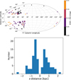 |
Fig. 1 Top: distribution of the non-composite HQS subdwarfs in Galactic coordinates, colour-coded with the monochromatic interstellar reddening parameter E(44−55) (see Sect. 5.2). Bottom: histogram of distances from the Galactic plane z for all stars with parallax errors better than 25% calculated from their Gaia parallaxes (see Sect. 2.4 for details). |
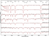 |
Fig. 2 Example spectral fits (red) to DSAZ spectra (black) of the main types of hot subdwarfs in HQS. |
2 Observational data and sample selection
This study is based on optical spectra (Sect. 2.1), time series photometry (Sect. 2.2), photometric measurements from the ultraviolet to the infrared regime (Sect. 2.3), and parallaxes from Gaia DR3 (Sect. 2.4).
2.1 Spectroscopic observations and classification
Optical spectra were obtained over 14 observing runs at the DSAZ, Calar Alto observatory in Spain between 1989 and 1998, using the TWIN spectrograph mounted at the 3.5 m telescope and CAFOS at the 2.2 m, which provided spectral resolutions from 3.4 Å to 8.0 Å (for details see Table 1 of Edelmann et al. 2003). Their signal-to-noise ratio ranges from 17 to 160 at a median of 56. Additional medium-resolution DSAZ spectra were taken from Silvotti et al. (2002) and Dreizler et al. (2002). The DSAZ spectra are complemented by data retrieved from the SDSS DR17 (Almeida et al. 2023) and LAMOST DR10 (Yan et al. 2022) databases, available for ≈ 30% of the sample, only.
Nine sdB stars, including six non-composite ones, were also observed at high spectral resolution (R=18 500 or better, Lisker et al. 2005) with UVES at the ESO VLT at two epochs each. Three were found to be radial-velocity variable (Napiwotzki et al. 2004). These spectra were analysed in the same way as the low-resolution spectra.
Rather than attempting to classify the individual spectra in a classical procedure (Moehler et al. 1990; Drilling et al. 2013; Geier et al. 2024)1, we used the derived Teff to formally distinguish sdB (Teff=20–30 kK), sdOB (Teff=30–40 kK), sdO (>40 kK) stars, and the derived log [n(He)/n(H)] to separate the sample into three helium categories: He-poor, intermediate He-rich (iHe), and extremely He-rich (eHe) subdwarfs. Here, we include nine categories. It has become common practice to distinguish an iHe from an eHe subdwarf at an abundance of n(He/H)=4 (see Heber 2016). The solar helium abundance has traditionally been used to tell He-rich and He-poor subdwarfs apart. However, recent studies by Latour et al. (2026) and Dawson et al. (2026) have shown this limit to be somewhat lowered from the solar value (log [n(He)/n(H)]=−1.0) to log [n(He)/n(H)]=−1.2, as in this paper. Example spectra of HQS subdwarfs for all subtypes are shown in Fig. 2.
2.2 Photometric variability, pulsations, and binarity
A significant fraction of hot subdwarfs show photometric variability due to pulsations, binarity, or – on occasion – both effects simultaneously. Many of the hot subdwarfs from the HQS have been followed-up with time series photometry to identify such variability effects. We reviewed the literature to identify the variable stars in our sample, and we retrieved photometric data from the Zwicky Transient Facility (ZTF; Bellm 2014) to search for additional large-amplitude variables (see Appendix A).
Pulsations. Multi-periodic radial and non-radial pulsations were observed in hot subdwarfs. Two types of pulsation can be distinguished: p-modes for which the restoring force is the pressure force, and g-modes with buoyancy as the restoring force (see Aerts 2021, for a review). The observed oscillation periods of p-modes are short (a few minutes) and longer for g-modes (≈45−250 min). P-mode pulsators are found at higher Teff(≈28 000−36 000 K), while g-mode pulsators are somewhat cooler (22 000–30 000 K). Hybrid pulsators showing both p-mode and g-mode pulsations are found mostly at intermediate temperatures. Ten p-mode pulsators and nine g-mode pulsators were found among the HQS subdwarfs. More details are given in Appendix A.
Binarity: Reflection effect and eclipsing hot subdwarf. Eight close binaries with late-type main-sequence companions are known among the HQS subdwarfs and exhibit a reflection effect; two are also eclipsing systems. The analysis of the ZTF light curves, presented in Appendix A, confirms all eight previously known cases but reveals no additional objects with detectable photometric variability. In four of the reflection-effect binaries, contamination of the optical spectra by the companion was found to be too severe; these systems were therefore excluded from the sample.
2.3 Multi-wavelength photometry
Photometric measurements were obtained by querying several public databases (see Culpan et al. 2024; Schneider et al. 2025, for a list of the photometric surveys used) and were used to construct SEDs (see Sect. 5). Hot subdwarfs in binaries with F-, G-, K-type main-sequence companions are easy to detect because their SEDs are composite. The subdwarf dominates the blue part, while the cool star contributes in the red and infrared part (see Sect. 5.1). The analysis of the 29 composite spectrum binaries, known from the literature and identified in the course of our analyses (see Sect. 5.1), is beyond the scope of this paper. We also excluded those close binary systems with the strong reflection effects mentioned in the previous subsection, because their strong light variations indicate that the optical spectra might be contaminated by light scattered back from the companion.
2.4 Gaia astrometry
Gaia parallaxes (Gaia Collaboration 2016, 2023) provide the stellar distances, which are crucial to derive stellar parameters. Because some stars are far away, their parallaxes are small. Moreover, their relative uncertainties are large; they strongly increase with decreasing parallax. From Fig. 3 we infer that for about 70% of the sample the uncertainties are smaller than 10%, and for 90% of the sample they are lower than 25%. The distance distribution peaks at 1.5 kpc with the nearest object at ≈ 600 pc (Fig. 3). The most distant stars lie beyond 5 kpc.
2.5 The selected sample of hot subdwarfs from the HQS
Our final sample of non-composite hot subdwarfs amounts to 122 stars. About two thirds of them are hydrogen-rich and one third is helium-rich. While the sdBs have been studied before, similar quantitative spectral analyses of the spectra of the He-rich hot subdwarfs have not been published. Seven stars were excluded from the sample because their spectral type turned out to be unrelated to the EHB after performing the spectral analyses (see Sect. 4.1). To derive stellar parameters, accurate parallaxes are required. We considered stars with relative parallax uncertainties larger than 25% unreliable, leading us to investigate the stellar parameters for 103 hot subdwarf stars.
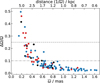 |
Fig. 3 Distribution of parallax uncertainties as a function of parallax. The dot-dashed and dashed lines mark the 10% and 25% uncertainty levels, respectively. HS0941+4649 and HS1000+4704 are off the scale; their parallax uncertainties are larger than the parallax. He-poor stars are shown in blue, iHe rich ones in black, and eHe-rich in red. |
3 2nd generation Bamberg models: Hybrid LTE/NLTE model atmospheres and synthetic spectra
Previously, metal-line-blanketed LTE model atmospheres (Heber et al. 2000) and metal-free NLTE models (Stroeer et al. 2007) or combinations thereof (Edelmann et al. 2003; Lisker et al. 2005) were used in many studies by our team (see Heber 2016). Through the last decade, we developed large grids of model atmospheres and synthetic H/He line spectra that combine metal-line blanketing and NLTE effects in an approximate way (Przybilla et al. 2011) to cover the entire parameter space of the hot subdwarfs homogeneously. These 2nd generation Bamberg model grids of hybrid LTE/NLTE atmospheres cover a wide range of atmospheric parameters (see Fig. 4). Because the He abundances of hot subdwarfs vary by seven orders of magnitudes from star to star, grids were calculated to cover the entire range.
In short, our approach made use of the LTE code ATLAS 12, the NLTE code DETAIL, and the spectrum synthesis code SURFACE. The metal composition of hot subdwarfs is far from solar but shows a characteristic pattern, where low mass elements are underabundant, while heavier elements such as the iron group are overabundant (Pereira 2011; Geier 2013). Our model atmosphere calculations used the mean abundance pattern derived by Pereira (2011), as reported by Naslim et al. (2013). The ATLAS 12 code (Kurucz 2013) was used to compute the atmospheric structure in LTE with the most recent Kurucz line lists to incorporate the line blanketing effect with the opacity sampling technique based on the mean chemical abundance patterns of hot subdwarfs. The hydrogen, He I, and He II line spectra were calculated with the DETAIL (Giddings 1981; Butler & Giddings 1985) and SURFACE codes (Butler & Giddings 1985), enabling departure from LTE. Recently, all three codes were modified (see Irrgang et al. 2018, 2021, for details) to incorporate the occupation probability formalism (Hummer & Mihalas 1988) for level dissolution. Consistent line broadening tables for hydrogen (Tremblay & Bergeron 2009) were incorporated. Both modifications are important to model the confluence of lines near the Balmer jump (Inglis & Teller 1939). Helium line broadening was improved by implementing the corrected tables from Beauchamp et al. (1997), Gigosos & González (2009), and Lara et al. (2012). A rigorous treatment of NLTE effects on the atmospheric structure is not possible in the ADS (ATLAS/DETAIL/SURFACE) approach. However, ATLAS 12 offers the opportunity to include departure coefficients calculated for small model atoms of hydrogen and helium with DETAIL and passed back to ATLAS 12, refining the atmospheric structure iteratively. This allowed us to incorporate NLTE effects on the atmospheric structure in an approximate way.
To account for the diverse abundance patterns of individual subdwarfs, H/He spectral grids are also available for the mean pattern scaled by factors of 1/100, 1/10 and 10 (henceforth z=−2, −1, 0, +1, on a logarithmic scale). The 2nd generation Bamberg model grids have been used recently by, for example, Geier et al. (2024), Latour et al. (2026), and Dawson et al. (2026).
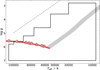 |
Fig. 4 Model atmosphere grid dimension in the Teff−log g plane (black line). The grey band denotes the EHB for solar composition (Dorman et al. 1993) for comparison. The helium main sequence (Paczyński 1971) is shown in red with masses labelled. The dashed line shows the Eddington limit for solar composition (Lamers & Fitzpatrick 1988). Grids are constructed at metal compositions of 1/100, 1/10, 1 and 10 times the standard sdB metallicity pattern and n(He)/n(H) of 1/10 000 to ≈100 times solar, depending on metal content. |
3.1 Spectral analysis procedure
We used a global fitting procedure developed by Irrgang et al. (2014), which replaced the previously used selective χ2 minimisation technique (Napiwotzki 1999; Hirsch 2009). The full spectral range, usually from 3600 or 3700 Å to 7300 Å, was used rather than pre-selecting spectral lines. Interstellar lines, such as the Ca II, H and K, and the Na I D lines, as well as artefacts were automatically excluded. The continuum was modelled with an Akima spline (Akima 1970) anchored at preselected intervals. The entire multi-parameter space (effective temperature, surface gravity, helium abundance, projected rotational velocity, and radial velocity) was fitted simultaneously with the continuum. Poorly fitting spectral regions were automatically excluded. Because of the low spectral resolution of the TWIN and CAFOS spectra, the projected rotation velocities were uncertain but consistent with zero. We note that the same procedure was applied by Dawson et al. (2026) and Latour et al. (2026) to the sample of nearby hot subdwarfs (volume complete to 500 pc) and the Arizona–Montréal sample, respectively. If multiple spectra were available, they were fitted simultaneously. To ensure homogeneity, we restricted ourselves to spectra that cover the Balmer jump to at least 3700 Å.
The atmospheric parameters are not independent but correlated. The most important correlation among them is between the effective temperature and gravity. We calculated covariance matrices and confidence maps and derived the correlation coefficients using the Cholesky-Banachiewicz decomposition algorithm (see Parthasarathy et al. 1995, and references therein) for the HQS sample. This correlation lies at the level of statistical uncertainties only, which means that the uncertainties are small on an absolute scale, including the correlations. The correlation is positive for all but the very hottest stars (see Fig. 5). It decreases with Teff both for the eHe rich sdOB/Os and for the He-poor subdwarfs, with the largest correlation factors at the lowest effective temperatures (20 kK and 40 kK, respectively). Fig. B.1 shows illustrative examples of confidence maps for different spectral types.
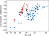 |
Fig. 5 Correlation of Teff with log g: Correlation factors as a function of Teff for He-poor (blue), iHe-rich (black), and eHe-rich subdwarfs (red). |
3.2 Systematic uncertainties
In addition to the statistical uncertainties from noise, systematic uncertainties also arise from different sources.
Intrinsic scatter. may be caused by limitations in the instrumental set-up, data reduction, and normalisation procedure. Repeated observations of the same star often scatter more than expected from statistical noise. In their investigation of sdB stars from the SPY project Lisker et al. (2005) studied the distributions of differences in atmospheric parameters between two exposures of ≈ 50 non-composite sdBs and found Δ Teff= 374 K, log g=0.049, and log [n(He)/n(H)]=0.044. Recently, Dawson et al. (2026) studied a larger sample based on low resolution spectra and found a polynomial representation of the intrinsic scatter with averages of 0.55% in Teff, 0.039 in log g, and 0.02 in log [n(He)/n(H)] for the main parameter ranges. We adopted the latter as a contribution to the systematic uncertainties of the atmospheric parameters, because they are based on spectra of resolutions similar to the DSAZ spectra.
Metallicity effect. Another uncertainty arises from the unknown metallicity of the individual stars. Ultraviolet line blocking is dominated by the high number of iron and nickel lines, responsible for most of the metal-line blanketing effect on the atmospheric temperature and density stratification. Since the strength of the lines depends on element abundance, their impact does as well. From high-resolution studies (e.g. O’Toole & Heber 2006; Blanchette et al. 2008), we know that the average Fe abundance is nearly solar, while Ni is about ten times solar in hot subdwarf stars. However, the abundances vary significantly from star to star by about ± 0.3 dex (1σ, Geier 2013). To account for these uncertainties, we repeated the fitting procedure for enhanced (z=+0.3) and depleted (z = −0.3) metal contents (see Sect. 3). This variation leads to systematic uncertainties on the atmospheric parameters, which we plot in Fig. 6 and Fig. C.12. These systematic uncertainties differ strongly among subtypes. While for helium poor subdwarfs the Teff uncertainties are larger than for He-rich ones, the opposite holds for log g. The He-rich stars show absorption lines from both neutral and ionised helium, allowing the ionisation equilibrium to constrain Teff more precisely than for the He-poor stars, which lack this information. On the other hand, the determination of surface gravity is largely based on the Stark-broadened Balmer and helium lines as well as the level-dissolution of high-lying H levels. The effect is more pronounced for the hydrogen Balmer line than for the helium line profiles. For the helium-to-hydrogen ratio (log [n(He)/n(H)]), the effect remains weak over a large range of values, while it is strong for both very low and very high He abundances. For low values, the He lines are very weak or absent, while at the high end the hydrogen Balmer line contribution to the blend with He ii is very small.
The additional contributions to the systematic uncertainties resulting from metallicity uncertainty  (for j=Teff, log g, log [n(He)/n(H)]) were added along with the observational (intrinsic δi,j) ones in quadrature to the statistical (δs,j) ones, which defines the adopted total uncertainty of the atmospheric parameters:
 where δi,j is the same for all stars.
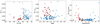 |
Fig. 6 Metallicity impact for the determination of atmospheric parameters for Teff, log g, and log [n(He)/n(H)] (left to right). Shown are half the maximum differences between parameters derived using models with standard metal composition and those with z= ± 0.3, for helium-poor (blue), helium-rich (red), and intermediate-helium (black) hot subdwarfs. For Teff the relative differences are shown. |
3.3 The impact of the 2nd generation Bamberg model approach: Revisiting the sdB stars in the HQS
To quantify the impact of the new model grid and analysis procedure, we revisited the sample of sdB stars from the HQS survey. Edelmann et al. (2003) analysed the same spectra using a mix of metal-line blanketed LTE atmospheres and NLTE model atmospheres, applying the former to stars cooler than Teff=27 000 K, the latter to stars hotter than Teff=35 000 K, and the mean of both for intermediate temperatures. Selected spectral lines of He and H were used to derive the atmospheric parameters. We compare their results to our new results from the homogeneous hybrid LTE/NLTE model grid and the global analysis strategy in Fig. 7, based on the same observations.
The new results are systematically different from the previously published ones, as demonstrated in Fig. 7. The Teff difference increases with the revised Teff, as shown in the left panel. A linear regression gives
![Mathematical equation: $T_{\text {eff}}^{{new}}=1.26 \times T_{\text {eff}}^{\text {publ}}-8\ [\mathrm{kK}],$](/articles/aa/full_html/2026/04/aa58636-25/aa58636-25-eq3.png) valid for temperatures between 25 kK and 40 kK. This can be traced back to the model grids used in the previous analysis. The new grid treats metal-line blanketing and departures from LTE in a homogeneous way, while the previous analysis uses a mix of model grids, as explained above. Some outliers are evident in the surface gravity values, but no clear trend is observed. On average, the revised values are higher than the previous ones by 0.08 dex. The revised helium abundances are lower by 0.08 dex. These results can be used to convert published results for sdB stars based on the old models (e.g. Maxted et al. 2001; Lisker et al. 2005; Morales-Rueda et al. 2003; Copperwheat et al. 2011; Geier et al. 2011, and many more) to the new scale.
valid for temperatures between 25 kK and 40 kK. This can be traced back to the model grids used in the previous analysis. The new grid treats metal-line blanketing and departures from LTE in a homogeneous way, while the previous analysis uses a mix of model grids, as explained above. Some outliers are evident in the surface gravity values, but no clear trend is observed. On average, the revised values are higher than the previous ones by 0.08 dex. The revised helium abundances are lower by 0.08 dex. These results can be used to convert published results for sdB stars based on the old models (e.g. Maxted et al. 2001; Lisker et al. 2005; Morales-Rueda et al. 2003; Copperwheat et al. 2011; Geier et al. 2011, and many more) to the new scale.
4 Results of the spectroscopic analyses
The sdO stars from the HQS survey follow-up have not been studied before. Because of their high helium abundance, both iHe and eHe subdwarfs stars show rich line spectra of neutral and ionised helium lines. Illustrative examples for spectral fits of the TWIN spectra of the iHe-sdOB HS 1837+5913, the eHe-sdOB HS 0836+6158, the iHe-sdO HS 1832+6955, and the eHe-sdO HS 1020+6926 are shown in Fig. 2. We must discuss some spectroscopically unusual stars, nonetheless, before we turn to the results for the full sample.
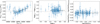 |
Fig. 7 Comparison of the effective temperatures (left), surface gravities (middle), and helium abundance (right) with those derived by Edelmann et al. (2003). The median values are indicated by a horizontal black line. |
4.1 Individual objects
A few sdO stars turned out to be very hot and/or of unusually low surface gravity. Although these stars are of great interest, we report only preliminary results in Table 1, as a sufficiently detailed investigation would require improved observations and additional atmospheric modelling.
4.1.1 Very hot stars
HS0216+0313 and HS1215+6247 (off-scale in Fig. 8) have effective temperatures exceeding 100 kK and high surface gravities (log g=>7.0 and 6.5, respectively). Because He II is detected at near solar abundance in both stars, they are likely DAO white dwarfs and, therefore, excluded from the sample.
4.1.2 Four post-AGB star candidates
The very hot He-rich sdO stars HS0237+0342, HS0657+5333, HS0736+3952, and HS1736+5521 have unusually low gravities (log g ≈ 5.2–5.4), indicating that they either belong to the rare group of He-rich, hot post-AGB stars, similar to the trio of stars LSE153, LSE259 and LSE263 (Husfeld et al. 1989; Krtička et al. 2024), though at somewhat higher gravity, or to the class of O(He) stars (Jeffery et al. 2023; Werner et al. 2025), though at somewhat lower Teff. Strong C iv lines are present in the spectra of the first three stars. Further investigations are necessary to draw firm conclusions. We therefore exclude them from the sample.
4.1.3 A possibly magnetic sdO star
HS0312+2225 is an iHe-sdO with a strong 4620 Å absorption feature. Because such a feature has been found in magnetic He-sdOs (Dorsch et al. 2024), we speculate that the star might be magnetic. However, no Zeeman splitting or broadening can be seen. HS0312+2225 has atmospheric parameters (Teff=45.5 kK, log g=5.95, log [n(He)/n(H)]=0), very similar to the known magnetic sdOs. High-resolution spectra are required to search for evidence of magnetism. We thus kept the star in the sample.
4.1.4 HS2123+0048, the central star of PN G053.9-33.2
This star has been suggested to be the central star of the planetary nebula G053.9-33.2 and marginally light-variable with a period of 2.546 d, possibly indicating an eclipsing binary (Aller et al. 2024). Further observations and modelling are required to improve the results. Although the object is very interesting, we exclude it from the sample here.
4.2 Kiel diagram and helium abundance distribution
Results from our spectral analysis are listed in Tables D.1 and D.2 and displayed in Fig. 8 via the Teff−log g (Kiel) and Teff−log [n(He)/n(H)] diagrams. The observed positions in the Kiel diagram are compared to predictions for the evolution of EHB stars (Dorman et al. 1993). Growing evidence shows that the distribution of stars along the EHB band is not homogenous (Németh et al. 2012; Geier et al. 2022; He et al. 2025). Geier et al. (2022) defined three different structures named EHB1 (cool end, Teff<25 kK), EHB2 (moderate Teff), and EHB3 (hot end, Teff > 33 kK); sdB and sdOB stars lying beyond or below the EHB band were named post-EHB and bEHB, respectively. Most of the He-poor sdB and sdOB stars in our HQS sample lie within the predicted core helium-burning EHB band, but only four sdBs, belonging to the EHB1 group, are found to be cooler than 25 000 K. The surface gravities for some He-poor sdBs and sdOBs are lower than predicted for the EHB band, which hints at a more evolved He-shell burning state. He-poor stars are also found among the sdO stars at temperatures well beyond the hot end of the EHB. They must have evolved even further towards the white dwarf cooling sequence. Many eHe-sdOs are nearly hydrogen-free; at helium abundances exceeding log [n(He)/n(H)]=+2, hydrogen becomes undetectable in our spectra.
The distribution of He-rich stars differs significantly from the He-poor stars. Most cluster near the helium main sequence at masses significantly higher than the canonical mass for the core helium flash. Projecting their position onto the He-ZAMS of Paczyński (1971) would predict masses from 0.45 M⊙ to 1.0 M⊙. He-rich subdwarf stars have been proposed to originate from mergers of two helium white dwarfs in close binaries caused by gravitational wave emission (Webbink 1984; Iben & Tutukov 1984). Zhang & Jeffery (2012) and Yu et al. (2021) modelled the evolution of such mergers. As an example, Fig. 8 shows a track for a merger model of two He white dwarfs of 0.35 M⊙, ending up on the helium main sequence in the region where the He-rich sdOs are found. Because the mass of a He white dwarf may be as high as 0.45 M⊙, the merger products may be considerably more massive than half a solar mass, which is typically assumed for EHB stars.
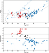 |
Fig. 8 Upper panel: Kiel diagram (Teff−log g). He-poor stars are indicated with blue circles, iHe subdwarfs with black circles, and eHe subdwarfs with red circles. The zero-age and terminal-age EHBs for a subsolar metallicity of −1.48 (solid grey lines) were interpolated from evolutionary tracks by Dorman et al. (1993). The helium main sequence (dashed line) is taken from Paczyński (1971). The evolution of a merging helium white dwarf (He-WD) system (Yu et al. 2021) is shown as a light blue line. Lower panel: helium abundance as a function of Teff. The lower and upper limits to log [n(He)/n(H)] are marked by upward and downward arrows. The iHe-rich subdwarfs are distinguished from the He-poor subdwarfs by the solid line, and from eHe-rich subdwarfs by the dashed line. |
5 Spectral energy distribution
Model grids of SEDs allow us to analyse photometric measurements from the FUV through the optical to the near- and mid-infrared (see Sect. 2.3). The synthetic flux distributions are calculated from the same model atmospheres used in the spectral analysis. The observed magnitudes were matched with synthetic SEDs keeping the atmospheric parameters fixed at the values determined from spectroscopy (see Heber et al. 2018, for details). Hence, the angular diameter Θ, and the interstellar colour excess E(44–55) remained as free parameters. The interstellar extinction was accounted for by using the function given by Fitzpatrick et al. (2019), assuming a standard monochromatic extinction coefficient of R(5500 Å)=3.02. The presentation of the flux distribution as fλ × λ3 in Fig. 9 eases the strong flux gradient towards the blue part of the SED. The SEDs of hydrogen-rich subdwarfs are characterised by the Balmer jump. Because of the lack of hydrogen, the Balmer jump is replaced by an absorption edge of He I in eHe-sdOBs (e.g. HS1843+6343), while in the hot sdOs (≳50 000 K) both edges vanish (see Fig. 9).
5.1 Detection of cool companions to hot subdwarfs from spectral energy distributions
F-, G-, or K-type companions to hot subdwarfs can easily be detected from the characteristic shape of their SED, where the blue part is dominated by the subdwarf and the red and infrared parts are dominated by the cool companion star. To detect late K- and early M-type companions, IR fluxes are crucial because their contributions in optical filters is very small. More than 80% of the sample have IR coverage, mostly from the 2 micron all sky survey (2MASS) (Cutri et al. 2003) and the UKIRT hemisphere survey (Schneider et al. 2025).
To model the flux distributions of cool companions, we interpolated them in a grid of LTE Phoenix model spectra provided by Husser et al. (2013). This added additional parameters to the fitting routine. We fixed the surface gravity at log g=4.5 and the metallicity at the solar value; these parameters could not be constrained by the SED. This left us with the effective temperature of the cool star and the surface ratio as additional fit parameters.
We confirm the composite spectrum nature of the 18 spectrum sdB binaries identified by Edelmann et al. (2003) and the three found by Lisker et al. (2005) from spectroscopy. Another sdB, HS0016+0044, was identified as a spectroscopic binary by Girven et al. (2012), also confirmed by our SED analysis. In addition, we find IR excesses for five sdB stars. Displaying the SED as f × λ3 in Fig. 9 accentuates the flux contribution of F-, G-, and K-type stars, characterised by the bound-free absorption of H− (λ<1.4 μm) in the H band. HS0232+3155, HS1824+5745 (see Fig. 9), HS2151+0857, and HS2303+0152 host early K-type stars, whereas the IR excess of HS1813+7247 is very weak and the companion does not contribute at optical wavelengths. The companion is an early M-type star, and we kept the star in our sample. HS1813+7247 further shows light variations indicating that it is a g-mode pulsator (TIC 229593795; Uzundag et al. 2024). Among the other HQS pulsating hot subdwarfs identified in the literature (see Sect. 2.2), we found that the p-mode pulsators HS1824+5745 (LS Dra), HS2303+0152, and HS2151+0857 are also composite spectrum objects (see Fig. 9) and hence excluded from our final sample.
Among the sdO stars, we identified two composite objects, HS0735+4026 and HS2308+0942. The IR excess of the former is weak, and we kept that star in the sample.
It is worth noting that 15 of our targets lack infrared H and K magnitude measurements. Consequently, a slight IR excess (as for HS1813+7247) may not be detected in our analysis of the stars.
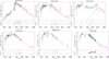 |
Fig. 9 Fits of the SEDs of selected programme stars. Each plot consists of two panels. Upper panel: observed fluxes compared to the synthetic SED. To ease the slope of the distribution, the flux fλ is multiplied by the wavelength to the power of three. Photometric fluxes are displayed as coloured data points with their respective uncertainties and filter widths (dashed lines). The best-fit models are drawn as full-drawn grey lines. Lower panels: uncertainty-weighted residuals χ demonstrating the quality of the fit. The 2200 Å bump in the interstellar extinction curve clearly appears in significantly reddened objects. Top row: He-poor hot subdwarfs (from left to right) – sdB HS2229+2628, sdOB HS2225+2220, and composite sdB pulsator HS1824+5745. Bottom row: single He-sdOB/O stars (from left to right) – eHe sdOB HS1843+6343, eHe sdO HS0019+3944, and iHe-sdO HS1832+6955. |
5.2 Interstellar reddening
Interstellar reddening as derived from the SED fit is found to be significant for most stars; its distribution on the sky is shown in Fig. 1. The high reddening between the Galactic longitudes l=150° and 190° at southern Galactic latitudes is caused by the Taurus-Perseus-California complex of the Gould belt (Alves et al. 2020). We compared the results to the line-of-sight reddening maps of Schlegel et al. (1998) and Schlafly & Finkbeiner (2011) and find our results to be consistent with the predictions of the maps.
6 Stellar parameters from spectral energy distributions and parallaxes
Radii, luminosities, and masses were derived by combining the atmospheric parameters determined in Section 4 with angular diameters and Gaia DR3 parallaxes (Gaia Collaboration 2023). Parallax zero-point offsets were corrected following Lindegren et al. (2021). The relative parallax uncertainties (δϖ) increase rapidly with decreasing parallax, as illustrated in Fig. 3. Stars with δ ϖ ≥ 25 per cent were excluded from the analysis. As such, large uncertainties led to unreliable stellar parameters. The re-normalised unit weight error (RUWE) is a quality control parameter that should be below 1.4 for good astrometric solutions (El-Badry et al. 2021). Thresholds on RUWE depend on the position of the object on the sky because of Gaia’s scanning law (Castro-Ginard et al. 2024). All stars in our sample have RUWE <1.2 and therefore pass this astrometric quality criterion, except for HS2233+1418 (RUWE =1.52), which is excluded from the analysis. This leaves a final sample of 103 stars for which stellar parameters were derived.
Absolute stellar radii, luminosities, and masses were computed through the basic relations
 (1)
where Θ is the angular diameter, ϖ the parallax, G is the gravitational constant, and σSB is the Stefan-Boltzmann constant.
(1)
where Θ is the angular diameter, ϖ the parallax, G is the gravitational constant, and σSB is the Stefan-Boltzmann constant.
We employed a Monte Carlo (MC) method to assess the uncertainties of error propagation from the input parameters Teff, log g, ϖ and log Θ, represented by Gaussian distributions. The correlation of Teff and log g was applied to the systematic uncertainties as well but had very little impact on the resulting stellar masses (Δ M<0.005 M⊙) (see Sect. 3.1). For each star, 106 samples were generated, with each array carried through the full calculation to the final derived parameter. The results listed in Table D.1 allow us to construct arguably the most important diagrams to test stellar evolution – that is, the physical HRD (Teff, log L) and the mass distribution.
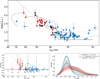 |
Fig. 10 HRD and mass distributions. Upper panel: HRD (Teff−logL). The dashed grey and dotted lines mark the standard EHB band for a metallicity of −1.48 (Dorman et al. 1993). The horizontal dashed black line at log L=1.05 marks the luminosity limit separating bEHB stars from EHB stars (see Dawson et al. 2026). While the lowest luminosity stars HS2029+0301 and HS2240+0136 lie on this line, none of the other stars lie below it. Lower left: mass vs. Teff. Helium-poor stars are marked in blue, extremely helium-rich sdOB and sdO stars in red, and iHe stars in black. Lower right: MC mass distribution as normalised KDEs for the three He subclasses. The shaded bands denote the uncertainty ranges. |
6.1 The Hertzsprung-Russell (Teff, log L) diagram
Fig. 10 shows the HRD. The helium-poor stars mostly lie on the EHB band up to Teff=40 kK. At the hot end, some are found on the helium main sequence for half a solar mass. The He-rich stars mostly lie close to the HeMS at somewhat higher masses, irrespective of whether they belong to the iHe or eHe classes.
The structure of the EHB, already discussed in the context of the Kiel diagram, is also evident in the HRD. In particular, there is a pronounced scarcity of sdB stars at the cool end (EHB1).
In Dawson et al. (2026), the region below the canonical EHB is defined using the 0.45 M⊙ evolutionary tracks of Han et al. (2002), which correspond to a luminosity of log L/L⊙=1.05. Using a similar definition, Geier et al. (2022) and He et al. (2025) identified a distinct population of sdB stars referred to as bEHB or EHBb stars located below the canonical EHB band. This population is most prominent in Dawson et al. (2026) but also present in the sample of Latour et al. (2026). By contrast, no stars in our sample fall below the EHB luminosity limit. Two sdOB stars are located on the log L/L⊙=1.05 boundary, still consistent with degenerate core ignition. The absence of bEHB stars is also evident in the Kiel diagram.
The bEHB stars are believed to have evolved from intermediate mass progenitors of 2.0−2.5 M⊙ (e.g. Han et al. 2002), which ignite helium burning in non-degenerate conditions from relatively young stars. The lack of bEHB stars here may thus indicate that the HQS sample consists of an older stellar population than the other samples.
Mass properties by spectral type in our sample.
6.2 Mass distribution
The stellar mass, considered the most fundamental stellar parameter, is computed from Teff, log g, and the parallax. Since the beginning of the Gaia era, parallax ϖ has become a precise quantity, at least for sufficiently nearby stars (see Dawson et al. 2024). To derive the mass, the gravity must be well constrained, but the accuracy of the spectroscopic results is limited by systematic uncertainties of the order of 0.07 dex, which are difficult to overcome, even for high-quality data (see Sect. 3.2). In Fig. 10 we plot the derived masses as functions of Teff, by separating Hepoor (log [n(He)/n(H)]<−1.2), iHe (−1.2<log [n(He)/n(H)]< +0.6) and eHe subdwarfs (log [n(He)/n(H)]>+0.6). Because the sample is flux-limited, more luminous He-sdO stars are seen at longer distances and, therefore, have larger parallax uncertainties. They will benefit from improved parallaxes expected from Gaia DR4. While the average masses of the helium-poor stars do not change with Teff, those of the He-rich subdwarfs increase with increasing Teff, consistent with their position in the HRD. In the lower right panel of Fig. 10 we show the mass distribution from MC simulations, as normalised kernel density estimates (KDEs) with a bandwidth of 0.1 M⊙ for a clear comparison between subclasses.
Table 2 lists the average mass (M̄) as a weighted mean and the median mass (M̃) of the distributions for each individual spectral type, similar to the approach of Latour et al. (2026). We also provide the statistics by helium abundance for the He-poor, iHe, and eHe hot subdwarfs, representing the properties of the distributions shown in Fig. 10.
Helium-poor sdB and sdOB stars are the most numerous members of the sample. Both show very similar median values (0.46 and 0.45 M⊙, respectively) consistent with predictions of the canonical evolution theory (Dorman et al. 1993). Given that the width of their distributions (σ) is similar to the median of the individual mass uncertainties (Merr), the observed mass distribution is consistent with a narrow intrinsic distribution predicted by binary population synthesis models (BPS; Han et al. 2003).3 On the other hand, the mass distribution of the eHe-rich subdwarfs is very different from that of the He-poor hot subdwarfs. It is much broader, with 68% of the stellar masses falling between 0.48 and 1.05 M⊙ with a median value of 0.70 M⊙. Furthermore, it does not show a distinct peak (see Fig. 10). The mass distribution of the iHe subdwarfs is similar to that of the extreme ones (0.42–0.95 M⊙), at a lower median mass of 0.55 M⊙, which is still higher than that of the He-poor subdwarfs. The standard deviation σ is significantly larger than the typical uncertainty Merr for iHe- and eHe stars. This finding supports the He-WD merger scenario for He-sdO stars, for which BPS models predict a broad mass distribution with masses up to ≈ 0.9 M⊙.
Mass distribution of pulsating subdwarf B stars. The resulting mass distribution for the 15 non-composite pulsators is shown in Fig. 11 and compared to the distribution of the helium-poor sdBs and sdOBs, not known to pulsate. No difference in their mass distribution can be seen, and the median masses agree.
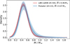 |
Fig. 11 Smooth mass distribution (normalised KDEs) for the non-composite pulsating sdB/sdOB stars (blue) from MC calculations. For comparison the mass distribution of the hot helium-poor subdwarf stars not known to pulsate is shown in red. The shaded bands denote the uncertainty ranges. |
7 Conclusions from comparison to similar studies
The conclusions drawn from the HQS sample may be compared to those of two studies using the same analysis strategy. The Arizona–Montréal sample (AM; Latour et al. 2026) is a magnitude-limited sample drawn mostly from the Palomar Green survey and thus comparable to the HQS sample, although it covers a larger area of sky at a shallower depth. The second study is a detailed analysis of the volume-complete sample of hot subdwarf stars within 500 pc presented by Dawson et al. (2026). In Fig. 12 we compare the mass distributions from the HQS to those from the AM and the 500 pc samples. The only volumelimited sample available is that of the hot subdwarfs within 500 pc. Because of the differences in brightness limits, there is no overlap between the HQS sample and the 500 pc sample and little (19 hot subdwarfs) with the Arizona-Montréal sample.
The results for the H-rich subdwarfs from all three samples are similar (see Table 3). There is no correlation of mass with Teff, with median masses of 0.45 (HQS), 0.465 (AM), and 0.48 M⊙(500 pc) close to the prediction of canonical evolution models. There is a significant difference concerning the presence of low mass subdwarfs evolving from intermediate mass progenitors (2–3 M⊙), which are present in both the 500 pc sample (10%) and to smaller fraction (6%) in the Arizona-Montréal sample, but are lacking in the HQS sample.
Masses for eHe-sdOs increase with increasing Teff in all samples, as predicted for He-MS stars. However, significant differences should be noted. In the 500 pc sample, the eHe-sdOs reaches nearly Teff=40 kK; only one star is hotter than 45 kK, and their median mass is lower (M̃=0.52 M⊙) than in the AM (M̃=0.76 M⊙) and the HQS sample (M̃=0.70 M⊙). Hence, there is a lack of hot massive eHe-sdOs in the 500 pc sample compared to those in the AM and HQS samples. It is also worthwhile to inspect the distribution along the He-MS. In the AM sample, the sequence appears to be evenly populated, while a gap appears to separate the lower near-canonical masses (0.5 M⊙) He-sdOs from the higher mass ones (0.7 to 1.0 M⊙). This gap is even more obvious in the HRD (Fig. 10).
Dawson et al. (2024) studied the space distribution of the 500 pc sample and derived a scale height of 281 ± 62 pc. A kinematical study by Dawson et al. (2026) showed that 90% of the sample belong to the thin disk population. Because the average distances of the stars above the plane in both the AM and HQS samples are longer than that scale height (see Fig. 1), we conclude that, on average, the AM and HQS hold populations of older stars than the volume-complete 500 pc sample. We speculate that, if eHe-rich subdwarfs indeed from from He-WD mergers, the more massive ones form in older populations than the less massive ones. Since the most massive He-WDs are formed in large red giants close to the tip of the RGB, the orbital periods of the post-CE double-He-WDs might be longer than the ones for the less massive He-WDs stripped in the subgiant stage. Since the merging time due to the emission of gravitational wave is a strong function of the orbital period, it might have taken the massive He-WD binaries longer to merge and form the He-sdOs we see now. The population of the 500 pc sample might therefore just be too young to form them.
Median masses and quantiles for mass distributions from the HQS sample compared to those from the Arizona-Montréal (AM, Latour et al. 2026), and the volume limited 500 pc sample (Dawson et al. 2026) grouped by He abundance.
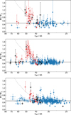 |
Fig. 12 Comparison of the mass distribution of the HQS sample (top) to the AM sample (middle, Latour et al. 2026) and that of the 500 pc sample (bottom, Dawson et al. 2026). He-poor stars are marked as blue circles, eHe-rich sdOB and sdO stars as red, and iHe stars as black ones. |
8 Summary and outlook
We studied 152 hot subdwarfs discovered in selected fields of the Hamburg Quasar Survey (HQS). The data include optical spectra, SEDs and Gaia DR3 astrometry. The stars are located in the northern and southern Galactic sky, mostly at intermediate Galactic latitudes. Because of the brightness limitations, the survey covers stellar distances from 600 pc up to a few kiloparsec, which probably includes both young and old stellar populations.
We detected low mass main-sequence companions of spectral type F, G, or K from their IR excess in 27 sdB/sdOB stars, of which 22 were already known and five sdBs were newly identified as composite binaries. We also discovered two new composite systems among the sdO stars, with HS0735+4026 being the only helium-rich subdwarf showing an IR excess in our survey. Light curves from the ZTF database revealed that four sdB binaries show periodic light variations due to reflected light from dM close companions. Because the amplitudes of their light variations were considered small, they were included in the sample for spectral analysis.
Low-resolution spectra of the non-composite systems taken at the Calar Alto observatory were analysed using extensive grids of hybrid LTE/NLTE model atmospheres and synthetic spectra (the 2nd generation Bamberg model grids) by making use of a global fitting strategy. Spectra were included only when they covered the blue part towards the Balmer jump to ensure that the spectral dataset was homogenous in terms of wavelength coverage. This allowed us to derive atmospheric parameters for 76 non-composite He-poor sdB/OB/O stars, 14 He-sdOB, and 26 He-sdO stars and compare them to predictions from evolutionary models in the Kiel diagram. In addition, we estimated atmospheric parameters for two very hot (>100 kK) DAO white dwarfs, four He-rich post-AGB stars, and one CSPN.
The sdB stars in the sample was analysed before with a mixed set of LTE and NLTE synthetic spectra (Edelmann et al. 2003). The comparison revealed a trend in between the new and old Teff results but constant offsets for the gravity and helium abundance. This information may be used to correct previously published results for the new Teff scale.
The sdB stars are found along the EHB band in all three previously discovered EHB substructures, with a low population in the coolest regime (EHB1). Most He-rich sdOB and sdO stars line up near the helium main sequence for masses between 0.5 and 1.0 M⊙.
The SEDs allowed us to determine stellar angular diameters and the interstellar extinction. In combination with Gaia parallaxes, the stellar parameters radius, luminosity, and mass were derived from the atmospheric parameters. The error budget for the latter is often dominated by systematic uncertainties. For the interpretation of the stellar parameters, we restricted the sample further to include stars with parallax uncertainties better than 25%, only. The resulting (Teff, log L) distribution (physical HRD) and the mass distribution consistently provide strong evidence that the He-poor hot subdwarfs have masses (0.45 M⊙) consistent with the canonical mass for the core helium flash of low mass RGB stars. We also provided atmospheric and stellar parameters for 15 known pulsating sdB stars and find no significant difference between their mass distribution and location in the physical HRD. In previous studies, (Geier et al. 2022; He et al. 2025) sdBs were found below the EHB band (bEHB), which harbour subdwarfs with masses less than canonical (<0.45 M⊙). We nonetheless found no bEHB star in the HQS sample.
The proximity of the He-rich sdOB and sdO stars to the helium main sequence is as obvious as in the Kiel diagram. The derived masses of He-rich sdOB stars (median 0.47 M⊙) are similar to those of the sdB stars, while the He-rich sdO stars are more massive (median 0.81 M⊙). Both results are consistent with the double helium white dwarf merger scenario. The He-rich sdO stars form the more massive and luminous part, and the He-rich sdOB stars form the lower mass and luminosity part of the sequence.
A comparison to similar studies such as AM sample (Latour et al. 2026) and 500 pc volume complete sample (Dawson et al. 2026) revealed mostly consistent results. Significant differences, however, are the absence of low mass subdwarfs evolving from intermediate mass progenitors (2–3 M⊙) in the HQS sample, present in both the 500 pc sample (10%) in the AM sample (6%). For the He-rich subdwarfs, significant differences appear in their mass distribution as well as location in the HRD. The most interesting is the lack of hot massive eHe-sdOs in the 500 pc sample compared to those in the AM and HQS samples. A gap in the HQS-eHe subdwarfs’ mass distribution – separating the lower near-canonical masses (0.5 M⊙) He-sdOs from the higher mass ones (0.7–1.0 M⊙) – is not found in the AM sample. We speculate that the more massive eHe-rich subdwarfs, which form from He-WD mergers, originate from older stellar populations than the less massive ones.
We excluded the composite spectrum binaries as well as some reflection effect systems from the study presented here. Those systems are important to understand the stable RLOF binary evolution channel for the formation of hot subdwarfs. We will apply the models and analysis strategy outlined here to those objects as well, which requires a larger parameter set to fit and additional observations.
Data availability
Tables D.1 and D.2 are available at the CDS via https://cdsarc.cds.unistra.fr/viz-bin/cat/J/A+A/708/A115.
Acknowledgements
We thank Andreas Irrgang for developing analysis tools. HD was supported by the DFG through grants GE2506/12-1, GE2506/17-1 and GE2506/9-2, FM through grant GE2506/18-1 and ML through grant LA4383/4-1. Based on observations collected at the Centro Astronómico Hispano Alemán (CAHA) at Calar Alto, operated jointly by the Max-Planck Institut für Astronomie and the Instituto de Astrofísica de Andalucía (CSIC). This work has made use of data from the European Space Agency (ESA) mission Gaia (https://www.cosmos.esa.int/gaia), processed by the Gaia Data Processing and Analysis Consortium (DPAC, https://www.cosmos.esa.int/web/gaia/dpac/consortium). Funding for the DPAC has been provided by national institutions, in particular the institutions participating in the Gaia Multilateral Agreement. Funding for the SDSS and SDSS-II has been provided by the Alfred P. Sloan Foundation, the Participating Institutions, the National Science Foundation, the U.S. Department of Energy, the National Aeronautics and Space Administration, the Japanese Monbukagakusho, the Max Planck Society, and the Higher Education Funding Council for England. The SDSS Website is http://www.sdss.org/. The SDSS is managed by the Astrophysical Research Consortium for the Participating Institutions. The Participating Institutions are the American Museum of Natural History, Astrophysical Institute Potsdam, University of Basel, University of Cambridge, Case Western Reserve University, University of Chicago, Drexel University, Fermilab, the Institute for Advanced Study, the Japan Participation Group, Johns Hopkins University, the Joint Institute for Nuclear Astrophysics, the Kavli Institute for Particle Astrophysics and Cosmology, the Korean Scientist Group, the Chinese Academy of Sciences (LAMOST), Los Alamos National Laboratory, the Max-Planck-Institute for Astronomy (MPIA), the Max-Planck-Institute for Astrophysics (MPA), New Mexico State University, Ohio State University, University of Pittsburgh, University of Portsmouth, Princeton University, the United States Naval Observatory, and the University of Washington. Funding for the Sloan Digital Sky Survey IV has been provided by the Alfred P. Sloan Foundation, the U.S. Department of Energy Office of Science, and the Participating Institutions. SDSS-IV acknowledges support and resources from the Center for High Performance Computing at the University of Utah. The SDSS website is www.sdss4.org. SDSI is managed by the Astrophysical Research Consortium for the Participating Institutions of the SDSS Collaboration including the Brazilian Participation Group, the Carnegie Institution for Science, Carnegie Mellon University, Center for Astrophysics, Harvard & Smithsonian, the Chilean Participation Group, the French Participation Group, Instituto de Astrofísica de Canarias, The Johns Hopkins University, Kavli Institute for the Physics and Mathematics of the Universe (IPMU)/University of Tokyo, the Korean Participation Group, Lawrence Berkeley National Laboratory, Leibniz Institut für Astrophysik Potsdam (AIP), Max-Planck-Institut für Astronomie (MPIA Heidelberg), Max-Planck-Institut für Astrophysik (MPA Garching), Max-Planck-Institut für Extraterrestrische Physik (MPE), National Astronomical Observatories of China, New Mexico State University, New York University, University of Notre Dame, Observatário Nacional/MCTI, The Ohio State University, Pennsylvania State University, Shanghai Astronomical Observatory, United Kingdom Participation Group, Universidad Nacional Autónoma de México, University of Arizona, University of Colorado Boulder, University of Oxford, University of Portsmouth, University of Utah, University of Virginia, University of Washington, University of Wisconsin, Vanderbilt University, and Yale University. Guoshoujing Telescope (the Large Sky Area Multi-Object Fiber Spectroscopic Telescope LAMOST) is a National Major Scientific Project built by the Chinese Academy of Sciences. Funding for the project has been provided by the National Development and Reform Commission. LAMOST is operated and managed by the National Astronomical Observatories, Chinese Academy of Sciences. The research has made use of TOPCAT, an interactive graphical viewer and editor for tabular data (Taylor 2005), of the SIMBAD database, and the VizieR catalogue access tool, both operated at CDS, Strasbourg, France.
References
- Aerts, C., 2021, Rev. Mod. Phys., 93, 015001 [Google Scholar]
- Akima, H., 1970, J. ACM, 17, 589 [Google Scholar]
- Aller, A., Lillo-Box, J., & Jones, D., 2024, A&A, 690, A190 [NASA ADS] [CrossRef] [EDP Sciences] [Google Scholar]
- Almeida, A., Anderson, S. F., Argudo-Fernández, M., et al. 2023, ApJS, 267, 44 [NASA ADS] [CrossRef] [Google Scholar]
- Alves, J., Zucker, C., Goodman, A. A., et al. 2020, Nature, 578, 237 [NASA ADS] [CrossRef] [Google Scholar]
- Aungwerojwit, A., & Gänsicke, B. T., 2009, in Astronomical Society of the Pacific Conference Series, 404, The Eighth Pacific Rim Conference on Stellar Astrophysics: A Tribute to Kam-Ching Leung, ed. S. J., Murphy, & M. S. Bessell, 276 [Google Scholar]
- Aungwerojwit, A., Gänsicke, B. T., Rodríguez-Gil, P., et al. 2005, A&A, 443, 995 [NASA ADS] [CrossRef] [EDP Sciences] [Google Scholar]
- Baran, A. S., Charpinet, S., Østensen, R. H., et al. 2024, A&A, 686, A65 [NASA ADS] [CrossRef] [EDP Sciences] [Google Scholar]
- Barlow, B. N., Corcoran, K. A., Parker, I. M., et al. 2022, ApJ, 928, 20 [NASA ADS] [CrossRef] [Google Scholar]
- Beauchamp, A., Wesemael, F., & Bergeron, P., 1997, ApJS, 108, 559 [NASA ADS] [CrossRef] [Google Scholar]
- Bellm, E., 2014, in The Third Hot-wiring the Transient Universe Workshop, eds. P. R. Wozniak, M. J. Graham, A. A. Mahabal, & R. Seaman, 27 [Google Scholar]
- Blanchette, J.-P., Chayer, P., Wesemael, F., et al. 2008, ApJ, 678, 1329 [NASA ADS] [CrossRef] [Google Scholar]
- Butler, K., & Giddings, J., 1985, Coll. Comp. Project No. 7 (CCP7), Newsletter, 9, 7 [Google Scholar]
- Castro-Ginard, A., Penoyre, Z., Casey, A. R., et al. 2024, A&A, 688, A1 [NASA ADS] [CrossRef] [EDP Sciences] [Google Scholar]
- Copperwheat, C. M., Morales-Rueda, L., Marsh, T. R., Maxted, P. F. L., & Heber, U., 2011, MNRAS, 415, 1381 [Google Scholar]
- Culpan, R., Dorsch, M., Geier, S., et al. 2024, A&A, 685, A134 [NASA ADS] [CrossRef] [EDP Sciences] [Google Scholar]
- Cutri, R. M., Skrutskie, M. F., van Dyk, S., et al. 2003, 2MASS All Sky Catalog of point sources [Google Scholar]
- Dawson, H., Geier, S., Heber, U., et al. 2024, A&A, 686, A25 [NASA ADS] [CrossRef] [EDP Sciences] [Google Scholar]
- Dawson, H., Dorsch, M., Geier, S., et al. 2026, A&A, 707, A6 [NASA ADS] [CrossRef] [EDP Sciences] [Google Scholar]
- Dorman, B., Rood, R. T., & O’Connell, R. W., 1993, ApJ, 419, 596 [NASA ADS] [CrossRef] [Google Scholar]
- Dorsch, M., Jeffery, C. S., Philip Monai, A., et al. 2024, A&A, 691, A165 [NASA ADS] [CrossRef] [EDP Sciences] [Google Scholar]
- Drechsel, H., Heber, U., Napiwotzki, R., et al. 2001, A&A, 379, 893 [NASA ADS] [CrossRef] [EDP Sciences] [Google Scholar]
- Dreizler, S., Werner, K., Jordan, S., & Hagen, H., 1994, A&A, 286, 463 [NASA ADS] [Google Scholar]
- Dreizler, S., Heber, U., Napiwotzki, R., & Hagen, H. J., 1995, A&A, 303, L53 [NASA ADS] [Google Scholar]
- Dreizler, S., Werner, K., Heber, U., & Engels, D., 1996, A&A, 309, 820 [NASA ADS] [Google Scholar]
- Dreizler, S., Schuh, S. L., Deetjen, J. L., Edelmann, H., & Heber, U., 2002, A&A, 386, 249 [NASA ADS] [CrossRef] [EDP Sciences] [Google Scholar]
- Drilling, J. S., Jeffery, C. S., Heber, U., Moehler, S., & Napiwotzki, R., 2013, A&A, 551, A31 [NASA ADS] [CrossRef] [EDP Sciences] [Google Scholar]
- Edelmann, H., Heber, U., Hagen, H.-J., et al. 2003, A&A, 400, 939 [NASA ADS] [CrossRef] [EDP Sciences] [Google Scholar]
- El-Badry, K., Rix, H.-W., & Heintz, T. M., 2021, MNRAS, 506, 2269 [NASA ADS] [CrossRef] [Google Scholar]
- Engels, D., Groote, D., Hagen, H. J., & Reimrs, D., 1988, in Astronomical Society of the Pacific Conference Series, 2, Optical Surveys for Quasars, eds. P. Osmer, M. M. Phillips, R. Green, & C. Foltz, 143 [Google Scholar]
- Enke, H., Tuvikene, T., Groote, D., Edelmann, H., & Heber, U., 2024, A&A, 687, A165 [NASA ADS] [CrossRef] [EDP Sciences] [Google Scholar]
- Er, H., Ozdonmez, A., Kenger, M. E., Gürbulak, B. B., & Nasiroglu, I., 2025, Adv. Space Res., 76, 1204 [Google Scholar]
- Fitzpatrick, E. L., Massa, D., Gordon, K. D., Bohlin, R., & Clayton, G. C., 2019, ApJ, 886, 108 [Google Scholar]
- Gaia Collaboration (Prusti, T., et al.,) 2016, A&A, 595, A1 [NASA ADS] [CrossRef] [EDP Sciences] [Google Scholar]
- Gaia Collaboration (Vallenari, A., et al.,) 2023, A&A, 674, A1 [NASA ADS] [CrossRef] [EDP Sciences] [Google Scholar]
- Gänsicke, B. T., Hagen, H. J., & Engels, D., 2002, in Astronomical Society of the Pacific Conference Series, 261, The Physics of Cataclysmic Variables and Related Objects, eds. B. T. Gänsicke, K. Beuermann, & K. Reinsch, 190 [Google Scholar]
- Geier, S., 2013, A&A, 549, A110 [NASA ADS] [CrossRef] [EDP Sciences] [Google Scholar]
- Geier, S., Maxted, P. F. L., Napiwotzki, R., et al. 2011, A&A, 526, A39 [NASA ADS] [CrossRef] [EDP Sciences] [Google Scholar]
- Geier, S., Østensen, R. H., Heber, U., et al. 2014, A&A, 562, A95 [NASA ADS] [CrossRef] [EDP Sciences] [Google Scholar]
- Geier, S., Heber, U., Irrgang, A., et al. 2024, A&A, 690, A368 [NASA ADS] [CrossRef] [EDP Sciences] [Google Scholar]
- Geier, S., Dorsch, M., Pelisoli, I., et al. 2022, A&A, 661, A113 [NASA ADS] [CrossRef] [EDP Sciences] [Google Scholar]
- Giddings, J. R., 1981, PhD thesis, University of London [Google Scholar]
- Gigosos, M. A., & González, M. Á. 2009, A&A, 503, 293 [NASA ADS] [CrossRef] [EDP Sciences] [Google Scholar]
- Girven, J., Steeghs, D., Heber, U., et al. 2012, MNRAS, 425, 1013 [CrossRef] [Google Scholar]
- Green, R. F., Schmidt, M., & Liebert, J., 1986, ApJS, 61, 305 [NASA ADS] [CrossRef] [Google Scholar]
- Groote, D., Heber, U., & Jordan, S., 1989, A&A, 223, L1 [Google Scholar]
- Hagen, H.-J., Groote, D., Engels, D., & Reimers, D., 1995, A&AS, 111, 195 [Google Scholar]
- Hagen, H. J., Engels, D., & Reimers, D., 1999, A&AS, 134, 483 [Google Scholar]
- Han, Z., Podsiadlowski, P., Maxted, P. F. L., Marsh, T. R., & Ivanova, N., 2002, MNRAS, 336, 449 [Google Scholar]
- Han, Z., Podsiadlowski, P., Maxted, P. F. L., & Marsh, T. R., 2003, MNRAS, 341, 669 [NASA ADS] [CrossRef] [Google Scholar]
- He, R., Meng, X., Lei, Z., Yan, H., & Lan, S., 2025, A&A, 693, A121 [NASA ADS] [CrossRef] [EDP Sciences] [Google Scholar]
- Heber, U., 2009, ARA&A, 47, 211 [Google Scholar]
- Heber, U., 2016, PASP, 128, 082001 [Google Scholar]
- Heber, U., 2024, arXiv e-prints [arXiv:2410.11663] [Google Scholar]
- Heber, U., Jordan, S., & Weidemann, V., 1991, in NATO Advanced Science Institutes (ASI) Series C, 336, NATO Advanced Science Institutes (ASI) Series C, eds. G. Vauclair, & E. Sion, 109 [Google Scholar]
- Heber, U., Dreizler, S., & Hagen, H.-J., 1996, A&A, 311, L17 [NASA ADS] [Google Scholar]
- Heber, U., Reid, I. N., & Werner, K., 2000, A&A, 363, 198 [NASA ADS] [Google Scholar]
- Heber, U., Drechsel, H., Østensen, R., et al. 2004, A&A, 420, 251 [NASA ADS] [CrossRef] [EDP Sciences] [Google Scholar]
- Heber, U., Irrgang, A., & Schaffenroth, J., 2018, Open Astron., 27, 35 [Google Scholar]
- Hirsch, H., 2009, PhD thesis, University of Erlangen-Nuremberg, http://www.sternwarte.uni-erlangen.de/Arbeiten/2009-07_Hirsch.pdf [Google Scholar]
- Homeier, D., & Koester, D., 2001, in Astronomical Society of the Pacific Conference Series, 226, 12th European Workshop on White Dwarfs, eds. J. L. Provencal, H. L. Shipman, J. MacDonald, & S. Goodchild, 397 [Google Scholar]
- Homeier, D., Koester, D., Hagen, H.-J., et al. 1998, A&A, 338, 563 [NASA ADS] [Google Scholar]
- Hummer, D. G., & Mihalas, D., 1988, ApJ, 331, 794 [NASA ADS] [CrossRef] [Google Scholar]
- Husfeld, D., Butler, K., Heber, U., & Drilling, J. S., 1989, A&A, 222, 150 [NASA ADS] [Google Scholar]
- Husser, T. O., Wende-von Berg, S., Dreizler, S., et al. 2013, A&A, 553, A6 [NASA ADS] [CrossRef] [EDP Sciences] [Google Scholar]
- Iben, I., J., & Tutukov, A. V. 1984, ApJS, 54, 335 [NASA ADS] [CrossRef] [Google Scholar]
- Inglis, D. R., & Teller, E., 1939, ApJ, 90, 439 [NASA ADS] [CrossRef] [Google Scholar]
- Irrgang, A., Przybilla, N., Heber, U., et al. 2014, A&A, 565, A63 [NASA ADS] [CrossRef] [EDP Sciences] [Google Scholar]
- Irrgang, A., Kreuzer, S., Heber, U., & Brown, W., 2018, A&A, 615, L5 [NASA ADS] [CrossRef] [EDP Sciences] [Google Scholar]
- Irrgang, A., Geier, S., Heber, U., et al. 2021, A&A, 650, A102 [NASA ADS] [CrossRef] [EDP Sciences] [Google Scholar]
- Jeffery, C. S., Miszalski, B., & Snowdon, E., 2021, MNRAS, 501, 623 [Google Scholar]
- Jeffery, C. S., Werner, K., Kilkenny, D., et al. 2023, MNRAS, 519, 2321 [Google Scholar]
- Krtička, J., Krtičková, I., Janík, J., et al. 2024, A&A, 683, A80 [NASA ADS] [CrossRef] [EDP Sciences] [Google Scholar]
- Krzesinski, J., & Balona, L. A., 2022, A&A, 663, A45 [NASA ADS] [CrossRef] [EDP Sciences] [Google Scholar]
- Krzesinski, J., Uzundag, M., Kumari, G. A., et al. 2025, A&A, 700, A71 [NASA ADS] [CrossRef] [EDP Sciences] [Google Scholar]
- Kupfer, T., Geier, S., McLeod, A., et al. 2014, in Astronomical Society of the Pacific Conference Series, 481, 6th Meeting on Hot Subdwarf Stars and Related Objects, eds. V. van Grootel, E. Green, G. Fontaine, & S. Charpinet, 293 [Google Scholar]
- Kurucz, R. L., 2013, ATLAS12: Opacity sampling model atmosphere program, Astrophysics Source Code Library [record ascl:1303.024] [Google Scholar]
- Lamers, H. J. G. L. M., & Fitzpatrick, E. L., 1988, ApJ, 324, 279 [CrossRef] [Google Scholar]
- Lara, N., González, M. Á., & Gigosos, M. A. 2012, A&A, 542, A75 [NASA ADS] [CrossRef] [EDP Sciences] [Google Scholar]
- Latour, M., Green, E. M., Dorsch, M., et al. 2026, A&A, 705, A248 [Google Scholar]
- Lemke, M., Heber, U., Napiwotzki, R., Dreizler, S., & Engels, D., 1997, in The Third Conference on Faint Blue Stars, eds. A. G. D. Philip, J. Liebert, R. Saffer, & D. S. Hayes, 375 [Google Scholar]
- Lindegren, L., Klioner, S. A., Hernández, J., et al. 2021, A&A, 649, A2 [EDP Sciences] [Google Scholar]
- Lipovetsky, V. A., Markarian, B. E., & Stepanian, J. A., 1987, in IAU Symposium, 121, Observational Evidence of Activity in Galaxies, eds. E. E. Khachikian, K. J. Fricke, & J. Melnick, 17 [Google Scholar]
- Lisker, T., Heber, U., Napiwotzki, R., et al. 2005, A&A, 430, 223 [NASA ADS] [CrossRef] [EDP Sciences] [Google Scholar]
- Luo, Y., Németh, P., Wang, K., Wang, X., & Han, Z., 2021, ApJS, 256, 28 [NASA ADS] [CrossRef] [Google Scholar]
- Luo, Y., Németh, P., Wang, K., & Pan, Y., 2024, ApJS, 271, 21 [NASA ADS] [CrossRef] [Google Scholar]
- Lutz, R., Schuh, S., Silvotti, R., et al. 2009, A&A, 496, 469 [NASA ADS] [CrossRef] [EDP Sciences] [Google Scholar]
- Mackebrandt, F., Schuh, S., Silvotti, R., et al. 2020, A&A, 638, A108 [NASA ADS] [CrossRef] [EDP Sciences] [Google Scholar]
- Markarian, B. E., Stepanian, J. A., & Erastova, L. K., 1987, in IAU Symposium, 121, Observational Evidence of Activity in Galaxies, ed. E. E. Khachikian, K. J. Fricke, & J. Melnick, 25 [Google Scholar]
- Marsh, T. R., 2018, in Handbook of Exoplanets, ed. H. J. Deeg, & J. A. Belmonte, 96 [Google Scholar]
- Maxted, P. F. L., Heber, U., Marsh, T. R., & North, R. C., 2001, MNRAS, 326, 1391 [CrossRef] [Google Scholar]
- Mengel, J. G., Norris, J., & Gross, P. G., 1976, ApJ, 204, 488 [Google Scholar]
- Moehler, S., Richtler, T., de Boer, K. S., Dettmar, R. J., & Heber, U., 1990, A&AS, 86, 53 [Google Scholar]
- Morales-Rueda, L., Maxted, P. F. L., Marsh, T. R., North, R. C., & Heber, U., 2003, MNRAS, 338, 752 [CrossRef] [Google Scholar]
- Napiwotzki, R., 1999, A&A, 350, 101 [Google Scholar]
- Napiwotzki, R., Karl, C. A., Lisker, T., et al. 2004, Ap&SS, 291, 321 [NASA ADS] [CrossRef] [Google Scholar]
- Naslim, N., Jeffery, C. S., Hibbert, A., & Behara, N. T., 2013, MNRAS, 434, 1920 [NASA ADS] [CrossRef] [Google Scholar]
- Németh, P., Kawka, A., & Vennes, S., 2012, MNRAS, 427, 2180 [Google Scholar]
- Østensen, R. H., Oreiro, R., Hu, H., Drechsel, H., & Heber, U., 2008, in Astronomical Society of the Pacific Conference Series, 392, Hot Subdwarf Stars and Related Objects, eds. U. Heber, C. S. Jeffery, & R. Napiwotzki, 221 [Google Scholar]
- Østensen, R. H., Oreiro, R., Solheim, J.-E., et al. 2010, A&A, 513, A6 [NASA ADS] [CrossRef] [EDP Sciences] [Google Scholar]
- O’Toole, S. J., & Heber, U., 2006, A&A, 452, 579 [CrossRef] [EDP Sciences] [Google Scholar]
- Paczyński, B., 1971, Acta Astron., 21, 1 [NASA ADS] [Google Scholar]
- Parthasarathy, M., Garcia-Lario, P., de Martino, D., et al. 1995, A&A, 300, L25 [NASA ADS] [Google Scholar]
- Pereira, C., 2011, PhD thesis, Queens University Belfast, Ireland [Google Scholar]
- Przybilla, N., Nieva, M.-F., & Butler, K., 2011, in Journal of Physics Conference Series, 328, Journal of Physics Conference Series (IOP), 012015 [Google Scholar]
- Pulley, D., Sharp, I. D., Mallett, J., & von Harrach, S., 2022, MNRAS, 514, 5725 [NASA ADS] [CrossRef] [Google Scholar]
- Rauch, T., Dreizler, S., & Wolff, B., 1998, A&A, 338, 651 [NASA ADS] [Google Scholar]
- Reimers, D., Koehler, T., & Wisotzki, L., 1996, A&AS, 115, 235 [Google Scholar]
- Reindl, N., Bainbridge, M., Przybilla, N., et al. 2019, MNRAS, 482, L93 [Google Scholar]
- Ricker, G. R., Winn, J. N., Vanderspek, R., et al. 2015, J. Astron. Telesc. Instrum. Syst., 1, 014003 [Google Scholar]
- Sahoo, S. K., Baran, A. S., Németh, P., et al. 2024, PASA, 41, e041 [Google Scholar]
- Sale, O., Bogensberger, D., Clarke, F., & Lynas-Gray, A. E., 2020, MNRAS, 499, 3071 [Google Scholar]
- Schaffenroth, V., Casewell, S. L., Schneider, D., et al. 2021, MNRAS, 501, 3847 [Google Scholar]
- Schaffenroth, V., Pelisoli, I., Barlow, B. N., Geier, S., & Kupfer, T., 2022, A&A, 666, A182 [NASA ADS] [CrossRef] [EDP Sciences] [Google Scholar]
- Schaffenroth, V., Barlow, B. N., Pelisoli, I., Geier, S., & Kupfer, T., 2023, A&A, 673, A90 [NASA ADS] [CrossRef] [EDP Sciences] [Google Scholar]
- Schlafly, E. F., & Finkbeiner, D. P., 2011, ApJ, 737, 103 [Google Scholar]
- Schlegel, D. J., Finkbeiner, D. P., & Davis, M., 1998, ApJ, 500, 525 [Google Scholar]
- Schneider, A. C., Vrba, F. J., Bruursema, J., et al. 2025, AJ, 170, 86 [Google Scholar]
- Schuh, S., Huber, J., Dreizler, S., et al. 2006, A&A, 445, L31 [NASA ADS] [CrossRef] [EDP Sciences] [Google Scholar]
- Silvotti, R., Janulis, R., Schuh, S. L., et al. 2002, A&A, 389, 180 [NASA ADS] [CrossRef] [EDP Sciences] [Google Scholar]
- Solheim, J. E., Østensen, R., Silvotti, R., & Heber, U., 2004, Ap&SS, 291, 419 [Google Scholar]
- Stark, M. A., & Wade, R. A., 2003, AJ, 126, 1455 [NASA ADS] [CrossRef] [Google Scholar]
- Stroeer, A., Heber, U., Lisker, T., et al. 2007, A&A, 462, 269 [NASA ADS] [CrossRef] [EDP Sciences] [Google Scholar]
- Taylor, M. B., 2005, in Astronomical Society of the Pacific Conference Series, 347, Astronomical Data Analysis Software and Systems XIV, eds. P. Shopbell, M. Britton, & R. Ebert, 29 [Google Scholar]
- Tremblay, P. E., & Bergeron, P., 2009, ApJ, 696, 1755 [Google Scholar]
- Uzundag, M., Vučković, M., Németh, P., et al. 2021, A&A, 651, A121 [NASA ADS] [CrossRef] [EDP Sciences] [Google Scholar]
- Uzundag, M., Krzesinski, J., Pelisoli, I., et al. 2024, A&A, 684, A118 [NASA ADS] [CrossRef] [EDP Sciences] [Google Scholar]
- Webbink, R. F., 1984, ApJ, 277, 355 [NASA ADS] [CrossRef] [Google Scholar]
- Werner, K., Dreizler, S., Heber, U., et al. 1995, A&A, 293, L75 [Google Scholar]
- Werner, K., Reindl, N., Pritzkuleit, M., & Geier, S., 2025, A&A, 693, A167 [NASA ADS] [CrossRef] [EDP Sciences] [Google Scholar]
- Wisotzki, L., Koehler, T., Groote, D., & Reimers, D., 1996, A&AS, 115, 227 [NASA ADS] [Google Scholar]
- Yan, H., Li, H., Wang, S., et al. 2022, Innovation, 3, 100224 [Google Scholar]
- Yu, J., Zhang, X., & Lü, G., 2021, MNRAS, 504, 2670 [NASA ADS] [CrossRef] [Google Scholar]
- Zhang, X., & Jeffery, C. S., 2012, MNRAS, 419, 452 [NASA ADS] [CrossRef] [Google Scholar]
Spectral atlases at ≈ 1 Å resolution are provided by Latour et al. (2026) and Jeffery et al. (2021) demonstrating their diversity.
A similar study was carried out by Dawson et al. (2026) for their volume-complete subdwarf sample; cf. their Fig. A.1.
We note that HS2033+0327 has a mass of 1.1 M⊙ but with large uncertainties (see Fig. 10). It is among the most distant sdBs in our sample. While this one star has little influence on the weighted average or the median mass of the sdBs, it strongly affects the standard deviation (σ). When removing the star, the σ of the sdB distribution is equal to 22%, thus fully consistent with that of the sdOB distribution.
Supplementary material
In Appendix A we present details about the pulsating stars in the HQS, results of the search for light variation, and the light curve analyses. Appendix B presents confidence maps of some subdwarfs representing different spectral subtypes used to derive the correlation coefficient r (see Sect. 3.1). The systematic uncertainties related to the uncertainty of the metal content has been discussed in Sect. 3.2. In Appendix C we demonstrate its impact on the Kiel diagram.
Appendix A Pulsating subdwarfs and reflection effect binaries
A photometric follow-up campaign provided light curves for 80 sdB stars from the HQS (Solheim et al. 2004; Østensen et al. 2010). The cadence of 20 seconds and observing time of 30 minutes were tailored to detect p-mode pulsators, which show multimode oscillations with periods between 1 and 6 minutes. Pulsations were found in ten out of the 80 surveyed stars (Østensen et al. 2010). Two of them, HS0702+6034 (DW Lyn) and HS2201+2610 (V391 Peg), show additional g-modes and are thus hybrid pulsators (Schuh et al. 2006; Lutz et al. 2009). Several of the HQS pulsators have been followed up to search for light travel time variations (e.g. Mackebrandt et al. 2020).
Observations by the Transiting Exoplanet Survey Satellite TESS (Ricker et al. 2015) have also been successfully analysed to identify new pulsators. The longer observing baselines provided by TESS is optimal for the detection of g-mode pulsations, which have longer periods and lower amplitudes than the p-mode pulsators. From the TESS data, four new HQS stars were found to have p-modes (Baran et al. 2024) and seven g-mode pulsators were identified (Uzundag et al. 2021; Krzesinski & Balona 2022; Uzundag et al. 2024; Sahoo et al. 2024). Furthermore, HS0212+1446 (TIC 58873368) and HS2233+2332 (TIC 242347840) are likely g-mode pulsators, but a binary nature could not be excluded (Uzundag et al. 2024) because only a single period could be detected for each star.
In addition to the pulsators, four short-period sdB binaries were discovered during ground-based campaigns, for which the light curves show a reflection effect caused by a close very low mass companion (dM or brown dwarf). Two of them are eclipsing systems of HW Vir type (HS0705+6700=V470 Cam, Drechsel et al. (2001), and HS2231+2441, Østensen et al. (2008)). For the former, eclipse time variations were detected indicating that it might have two circum-binary companions of low mass (Marsh 2018; Sale et al. 2020; Pulley et al. 2022, and references therein), as for the latter, it does not show any evidence of period variations from more than 18 years of eclipse timing measurements (Er et al. 2025). No eclipses were found for the two other systems HS2333+3927 (Heber et al. 2004) and HS2043+0615 (Geier et al. 2014). These four binaries were excluded from the spectral analysis because the reflection effect is quite large and their optical spectra may be contaminated by reflected light from the heated hemispheres of their companions (see e.g. Schaffenroth et al. 2021), which is phase-dependent.
Krzesinski et al. (2025) analysed TESS observations and found that HS2035+0418 (TIC 466750264) might be a reflection effect binary. Its period is short (0.1310 d) but the amplitude is small (see Fig. A.2 of Krzesinski et al. 2025). HS1741+2133 is a known close binary with a WD companion in a 0.2 d orbit (Kupfer et al. 2014). The TESS light curve showed ellipsoidal variations with a period of 4.78 h and an amplitude of ≈ 1 mmag (Schaffenroth et al. 2023). HS 1843+6953 and HS 1909+7004 were identified as additional candidate reflection effect systems by Schaffenroth et al. (2022) with periods of 8.08 h and 8.48 h, respectively, but small amplitudes. HS1320+2622 was found to be variable by Barlow et al. (2022), which we confirm from our ZTF light-curve analysis and we derived an orbital period of 0.1674 d. Because of their small light variations (see Fig. A.1) we keep those five stars in the sample.
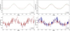 |
Fig. A.1 ZTF light curves in the g (blue) and r (red) bands of reflection effect systems phased to the corresponding orbital periods. Upper left: HS1843+6953 (P=0.3367 d). Upper right: HS1909+7004 (P=0.3537 d). Lower left: HS2035+0418 (P=0.1310 d). Lower right: HS1320+2622 (P=0.1674 d). No eclipses can be found for the other system. Note the different scales. |
We searched for other large-amplitude light variables in our sample by constructing light curves from the ZTF database. The ZTF is a ground-based photometric survey of the northern Hemisphere (Bellm 2014). ZTF periodically scans the entire northern Sky with a tree-day cadence, providing photometric data in the g and r bands with an approximately two-day cadence.
We combined all available photometric measurements from the ZTF survey, available for all but three stars of the sample, and used the lightkurve package for analysis. We recovered the known reflection effect systems (see Figs. A.1) but did not find indications for light variations in additional stars at amplitudes exceeding ≈ 0.01 mag and periods from 0.1 to 30 days.
Appendix B Correlation of temperature and surface gravity in the spectral analysis
The shape of the hydrogen and helium lines depends on temperature and density through atomic level excitation, ionisation and collisional line broadening, which yields a correlation between the effective temperature and gravity. To explore this correlation, we generated 2D χ2 confidence maps for all stars. We present some examples in Fig. B.1, demonstrating that the shape of the maps changes with helium content. The resulting correlation coefficients are plotted in Fig. 5. They were included in the systematic uncertainties as well and used in the error propagation to compute the uncertainties on the stellar parameters.
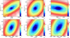 |
Fig. B.1 Confidence maps for atmospheric parameters derived from spectroscopy. Examples are selected to cover different spectral types. The contour lines refer to single parameter uncertainties of 68% (red contour) and 99.7% (black contour), respectively. Top row: He-poor sdB/O stars. The cool sdB, HS2218+0201 (correlation coefficient r=0.73), the sdOB star HS1806+5024 (r=0.36), and the hot sdO HS2123+0045(r = −0.52) are shown. Bottom row: He-rich sdOs. iHe sdO HS1832+6955 (r=0.37), eHe sdOB HS1843+6343 (r=0.70), and eHe sdO HS1638+6733 (r=0.56) are shown. |
Appendix C Systematic uncertainties due to metallicity differences
The effect of different metal content has been discussed in Sect. 3.2. Fig. C.1 demonstrates the effect on stars’ position in the Kiel-diagram and in the log [n(He)/n(H)] versus Teff plane.
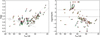 |
Fig. C.1 Impact of metallicity for the determination of atmospheric parameters in the Teff vs log g (left) and log [n(He)/n(H)] vs Teff (right) plane. Results derived for standard metal composition (z=0) are marked by blue crosses. The red and green symbols indicate the parameters derived for these same stars when fixing the metal content to half (z=−0.3) and twice (z=+0.3) the standard composition, respectively, and are connected by black lines to highlight the shifts. The position of the EHB band (dashed and dotted lines) and the zero-age helium main sequence (dot-dashed line, marked with the stellar mass) is also shown in the Teff vs log g plane. |
All Tables
Median masses and quantiles for mass distributions from the HQS sample compared to those from the Arizona-Montréal (AM, Latour et al. 2026), and the volume limited 500 pc sample (Dawson et al. 2026) grouped by He abundance.
All Figures
|
Fig. 1 Top: distribution of the non-composite HQS subdwarfs in Galactic coordinates, colour-coded with the monochromatic interstellar reddening parameter E(44−55) (see Sect. 5.2). Bottom: histogram of distances from the Galactic plane z for all stars with parallax errors better than 25% calculated from their Gaia parallaxes (see Sect. 2.4 for details). |
| In the text | |
|
Fig. 2 Example spectral fits (red) to DSAZ spectra (black) of the main types of hot subdwarfs in HQS. |
| In the text | |
|
Fig. 3 Distribution of parallax uncertainties as a function of parallax. The dot-dashed and dashed lines mark the 10% and 25% uncertainty levels, respectively. HS0941+4649 and HS1000+4704 are off the scale; their parallax uncertainties are larger than the parallax. He-poor stars are shown in blue, iHe rich ones in black, and eHe-rich in red. |
| In the text | |
|
Fig. 4 Model atmosphere grid dimension in the Teff−log g plane (black line). The grey band denotes the EHB for solar composition (Dorman et al. 1993) for comparison. The helium main sequence (Paczyński 1971) is shown in red with masses labelled. The dashed line shows the Eddington limit for solar composition (Lamers & Fitzpatrick 1988). Grids are constructed at metal compositions of 1/100, 1/10, 1 and 10 times the standard sdB metallicity pattern and n(He)/n(H) of 1/10 000 to ≈100 times solar, depending on metal content. |
| In the text | |
|
Fig. 5 Correlation of Teff with log g: Correlation factors as a function of Teff for He-poor (blue), iHe-rich (black), and eHe-rich subdwarfs (red). |
| In the text | |
|
Fig. 6 Metallicity impact for the determination of atmospheric parameters for Teff, log g, and log [n(He)/n(H)] (left to right). Shown are half the maximum differences between parameters derived using models with standard metal composition and those with z= ± 0.3, for helium-poor (blue), helium-rich (red), and intermediate-helium (black) hot subdwarfs. For Teff the relative differences are shown. |
| In the text | |
|
Fig. 7 Comparison of the effective temperatures (left), surface gravities (middle), and helium abundance (right) with those derived by Edelmann et al. (2003). The median values are indicated by a horizontal black line. |
| In the text | |
|
Fig. 8 Upper panel: Kiel diagram (Teff−log g). He-poor stars are indicated with blue circles, iHe subdwarfs with black circles, and eHe subdwarfs with red circles. The zero-age and terminal-age EHBs for a subsolar metallicity of −1.48 (solid grey lines) were interpolated from evolutionary tracks by Dorman et al. (1993). The helium main sequence (dashed line) is taken from Paczyński (1971). The evolution of a merging helium white dwarf (He-WD) system (Yu et al. 2021) is shown as a light blue line. Lower panel: helium abundance as a function of Teff. The lower and upper limits to log [n(He)/n(H)] are marked by upward and downward arrows. The iHe-rich subdwarfs are distinguished from the He-poor subdwarfs by the solid line, and from eHe-rich subdwarfs by the dashed line. |
| In the text | |
|
Fig. 9 Fits of the SEDs of selected programme stars. Each plot consists of two panels. Upper panel: observed fluxes compared to the synthetic SED. To ease the slope of the distribution, the flux fλ is multiplied by the wavelength to the power of three. Photometric fluxes are displayed as coloured data points with their respective uncertainties and filter widths (dashed lines). The best-fit models are drawn as full-drawn grey lines. Lower panels: uncertainty-weighted residuals χ demonstrating the quality of the fit. The 2200 Å bump in the interstellar extinction curve clearly appears in significantly reddened objects. Top row: He-poor hot subdwarfs (from left to right) – sdB HS2229+2628, sdOB HS2225+2220, and composite sdB pulsator HS1824+5745. Bottom row: single He-sdOB/O stars (from left to right) – eHe sdOB HS1843+6343, eHe sdO HS0019+3944, and iHe-sdO HS1832+6955. |
| In the text | |
|
Fig. 10 HRD and mass distributions. Upper panel: HRD (Teff−logL). The dashed grey and dotted lines mark the standard EHB band for a metallicity of −1.48 (Dorman et al. 1993). The horizontal dashed black line at log L=1.05 marks the luminosity limit separating bEHB stars from EHB stars (see Dawson et al. 2026). While the lowest luminosity stars HS2029+0301 and HS2240+0136 lie on this line, none of the other stars lie below it. Lower left: mass vs. Teff. Helium-poor stars are marked in blue, extremely helium-rich sdOB and sdO stars in red, and iHe stars in black. Lower right: MC mass distribution as normalised KDEs for the three He subclasses. The shaded bands denote the uncertainty ranges. |
| In the text | |
|
Fig. 11 Smooth mass distribution (normalised KDEs) for the non-composite pulsating sdB/sdOB stars (blue) from MC calculations. For comparison the mass distribution of the hot helium-poor subdwarf stars not known to pulsate is shown in red. The shaded bands denote the uncertainty ranges. |
| In the text | |
|
Fig. 12 Comparison of the mass distribution of the HQS sample (top) to the AM sample (middle, Latour et al. 2026) and that of the 500 pc sample (bottom, Dawson et al. 2026). He-poor stars are marked as blue circles, eHe-rich sdOB and sdO stars as red, and iHe stars as black ones. |
| In the text | |
|
Fig. A.1 ZTF light curves in the g (blue) and r (red) bands of reflection effect systems phased to the corresponding orbital periods. Upper left: HS1843+6953 (P=0.3367 d). Upper right: HS1909+7004 (P=0.3537 d). Lower left: HS2035+0418 (P=0.1310 d). Lower right: HS1320+2622 (P=0.1674 d). No eclipses can be found for the other system. Note the different scales. |
| In the text | |
|
Fig. B.1 Confidence maps for atmospheric parameters derived from spectroscopy. Examples are selected to cover different spectral types. The contour lines refer to single parameter uncertainties of 68% (red contour) and 99.7% (black contour), respectively. Top row: He-poor sdB/O stars. The cool sdB, HS2218+0201 (correlation coefficient r=0.73), the sdOB star HS1806+5024 (r=0.36), and the hot sdO HS2123+0045(r = −0.52) are shown. Bottom row: He-rich sdOs. iHe sdO HS1832+6955 (r=0.37), eHe sdOB HS1843+6343 (r=0.70), and eHe sdO HS1638+6733 (r=0.56) are shown. |
| In the text | |
|
Fig. C.1 Impact of metallicity for the determination of atmospheric parameters in the Teff vs log g (left) and log [n(He)/n(H)] vs Teff (right) plane. Results derived for standard metal composition (z=0) are marked by blue crosses. The red and green symbols indicate the parameters derived for these same stars when fixing the metal content to half (z=−0.3) and twice (z=+0.3) the standard composition, respectively, and are connected by black lines to highlight the shifts. The position of the EHB band (dashed and dotted lines) and the zero-age helium main sequence (dot-dashed line, marked with the stellar mass) is also shown in the Teff vs log g plane. |
| In the text | |
Current usage metrics show cumulative count of Article Views (full-text article views including HTML views, PDF and ePub downloads, according to the available data) and Abstracts Views on Vision4Press platform.
Data correspond to usage on the plateform after 2015. The current usage metrics is available 48-96 hours after online publication and is updated daily on week days.
Initial download of the metrics may take a while.