| Issue |
A&A
Volume 708, April 2026
|
|
|---|---|---|
| Article Number | A88 | |
| Number of page(s) | 11 | |
| Section | Extragalactic astronomy | |
| DOI | https://doi.org/10.1051/0004-6361/202558737 | |
| Published online | 26 March 2026 | |
Weak-emission-line quasar SDSS J101353.45+492758.1
I. Continuum fitting
1
Faculty of Physics, University of Białystok, ul. Ciołkowskiego 1L, 15-245 Białystok, Poland
2
Nicolaus Copernicus Astronomical Center, Polish Academy of Sciences, ul. Bartycka 18, Warsaw, Poland
3
National Centre for Nuclear Research, Astrophysics Division, ul. Pasteura 7, 02-093 Warsaw, Poland
★ Corresponding author: This email address is being protected from spambots. You need JavaScript enabled to view it.
Received:
22
December
2025
Accepted:
2
March
2026
Abstract
Context. Weak-emission-line quasars (WLQs) are active galactic nuclei (AGNs) characterized by unusually faint or absent broad emission lines. A subset also exhibits pronounced X-ray weakness, offering keys insights into accretion flow structure and the physical state of the broad-line region.
Aims. We present a broadband study of the WLQ SDSS J101353.45+492758.1, which displays a nearly featureless UV–optical spectrum with only a weak Mg II line alongside an exceptionally low X-ray flux.
Methods. We modeled its spectral energy distribution using the relativistic thin-disk model kerrbb with a power law and the multicomponent AGN model relagn, a physically motivated extension of agnsed that incorporates warm and hot Comptonizing regions. Our fits constrain the black hole (BH) mass, accretion rate, X-ray loudness, and coronal energetics.
Results. Both approaches yield consistent BH masses of MBH ≈ 2 × 10⁹ M⊙ and an Eddington accretion rate of ṁ ≈ 0.1. The relagn fit, which includes a warm Comptonizing region, provides a significantly improved representation of the UV-soft X-ray continuum. The warm corona, characterized by kTe ≃ 0.20 keV, Γ ≃ 3.8, and an optical depth τ ≃ 7.26, extends to ∼34 Rg. The hot corona appears compact and energetically suppressed, leading to an intrinsically weak X-ray output with log(LX/Lbol)≃ − 4.29, among the lowest reported for WLQs. The αOX ∼ 2.06 indicates the source is in a high (soft) AGN spectral state.
Conclusions. The combination of a luminous, standard disk and an extremely weak hot corona suggests that this quasar hosts a highly inefficient inner coronal region. This explains its X-ray faintness and extreme deficit of high-ionization emission lines. The source may represent an AGN analog in an “ultrasoft” accretion state, or a system in which the ionizing continuum is suppressed by a compact or quenched corona. Our study suggests that the source is not accreting at a high Eddington ratio, highlighting the physical diversity of WLQs, and supports the view that geometric and radiative effects jointly shape WLQs’ extreme spectral properties.
Key words: galaxies: active / galaxies: nuclei / quasars: emission lines / quasars: individual: SDSS J101353.45+492758.1
© The Authors 2026
 Open Access article, published by EDP Sciences, under the terms of the Creative Commons Attribution License (https://creativecommons.org/licenses/by/4.0), which permits unrestricted use, distribution, and reproduction in any medium, provided the original work is properly cited.
This article is published in open access under the Subscribe to Open model. This email address is being protected from spambots. You need JavaScript enabled to view it. to support open access publication.
1. Introduction
Strong and broad emission lines are hallmarks of the optical-UV spectra of active galaxies, especially quasars. However, various sky surveys have identified objects classified as quasars that exhibit weak or even undetectable emission lines – they are known as weak-emission-line quasars (WLQs; e.g., McDowell et al. 1995; Diamond-Stanic et al. 2009; Plotkin et al. 2010). Although WLQs share many characteristics with typical quasars (Shemmer et al. 2009), their optical-UV spectrum properties remain enigmatic. Their emission lines have significantly weaker equivalent widths (EWs) compared to classical quasars. For instance, the EW of the CIV emission line in WLQs is smaller than or equal to 10 Å, while in typical quasars its 1σ range spans from 26 to 67 Å (Diamond-Stanic et al. 2009). Broad emission lines can be divided into two categories (Wills et al. 1985; Collin-Souffrin & Lasota 1988). The first consists of high-ionization lines (HILs) emitted by a highly ionized low-density region of the broad-line region (BLR), including lines such as C IV and He II. The second category comprises low-ionization lines (LILs), which originate from a denser, less ionized region of the BLR or from a region farther from the ionizing source. This region produces, for example, the Mg II, Fe II, and hydrogen Balmer lines.
WLQs, though uncommon, pose a significant challenge to our current understanding of quasar structure and physics – particularly the nature of the BLR. Several hypotheses have been proposed to explain the physical origin of WLQs.
It was speculated that WLQs have intrinsically normal UV lines that appear weak because of dilution by a relativistically boosted continuum, similar to BL Lac objects. However, this is unlikely for most WLQs because they are radio-quiet sources (Plotkin et al. 2010).
Some authors have proposed that WLQs trace a youthful quasar stage, when the BLR has not yet fully formed (e.g., Hryniewicz et al. 2010; Andika 2020). While the accretion disk is already active and producing a standard continuum, the formation of the BLR is in progress. An alternative explanation suggested by Shemmer et al. (2010) is that the weak emission lines stem from a sparsely populated BLR with a noticeable deficit of line-emitting material. Moreover, Nikołajuk & Walter (2012) suggested that the low covering factor of the BLR could be responsible for the weakness of the emission lines.
The lack of sufficient high-energy ionizing photons is another direction to explore to understand the observed emission line weakness (Leighly et al. 2007). Such a soft spectral energy distribution (SED) could result from an atypical accretion rate. However, observations by Shemmer et al. (2010) have shown that two high-redshift WLQs have accretion rates typical of normal quasars with comparable luminosities and redshifts (a mean Eddington ratio of 0.35 was found by Shen et al. 2011, and a ratio of 0.4 was found by Shemmer).
Lastly, one might speculate that there is some material absorbing the ionizing photons (in the UV and X-ray energy bands) before they reach the BLR. Wu et al. (2011) studied a group of X-ray-weak quasars with UV emission line features similar to those of PHL 1811, including weak and blueshifted HILs. These PHL 1811 analogs have X-ray luminosities that are on average 13 times lower than expected, along with harder X-ray spectra, suggesting strong absorption. Interestingly, these analogs may constitute nearly 30% of WLQs. While early studies (e.g., Shemmer et al. 2009; Wu et al. 2011) emphasized X-ray weakness as a defining trait of WLQs, more recent works have suggested the presence of a shielding gas that selectively blocks high-energy photons from reaching the BLR (Wu et al. 2011; Luo et al. 2015; Ni et al. 2018). Such a shielding material geometry and orientation effects may play a key role. Depending on the observer’s line of sight, the same object might appear as a PHL 1811 analog (if viewed through the shielding gas and BLR) or as an X-ray-normal quasar. In this case, the mean ratio of the X-ray luminosity in the 0.5–10 keV range to the bolometric luminosity is 0.034, as calculated from 783 quasars based on the catalogs from Shen et al. (2011) and Young et al. (2009).
In this study we performed a broadband spectral analysis of the intriguing WLQ SDSS J101353.45+492758.1 (hereafter SDSS J101353). Section 2 provides a description of the quasar and outlines the data collection. In Sect. 3 we present the Mg II line analysis, including the measurement of the Mg II emission line. Section 4 is dedicated to the disk fitting method. We first detail the data corrections applied and then the procedure used to fit the SED of SDSS J101353. In Sect. 5 we explore another scenario: the obscuration and the reflection of X-rays as an alternative explanation for the X-ray faintness. The results, along with a discussion, are presented in Sect. 6, and conclusions are given in Sect. 7.
2. Quasar SDSS J101353.45+492758.1
2.1. The source description
With the aim of collecting a large sample of WLQs with redshift ranging from 0.19 to 3.50, we carefully examined the spectra of a dozen of WLQs from the Sloan Digital Sky Survey (SDSS) optical catalog data release 17 (DR17; Abdurro’uf et al. 2022). Among these selected quasars, the spectrum of SDSS J101353 retained our attention, showing a normal quasar spectrum (see Fig. 1), with almost no emission lines. Although weak, the Mg II emission line is clearly detected. However, the C IV and C III] emission lines are not clearly visible (see the spectrum in Fig. 2). Additionally, the quasar exhibits low level of X-ray radiation. Typical X-ray fluxes of luminous quasars lie around 10−14–10−13 erg cm−2 s−1 in the 2–10 keV energy band (e.g., Young et al. 2009). By contrast, SDSS J101353 is detected at FX ∼ 10−17 erg cm−2 s−1 – i.e., 103–104 times fainter than a typical quasar. Its X-ray luminosity in the 0.5–10 keV range estimated by Young et al. (2009) is 2.25 × 1041 erg s−1. SDSS J101353 is located at redshift z = 1.63558 ± 0.00128. Its coordinates are RA = 153.47276, Dec = 49.46615 (J2000.0). We cross-checked the redshift value based on the Mg II line using the SDSS interactive spectrum analyzer1. Using the+ online cosmology calculator2 developed by Wright (2006), we determined the comoving distance of SDSS J101353 to 4691.20 Mpc.
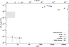 |
Fig. 1. Data points (black) and spectrum (blue; extracted from SDSS DR17) of SDSS J101353 in the observed frame. The light gray box represents the typical X-ray flux measured in the 2–10 keV energy band of classical quasars (e.g., Young et al. 2009). |
2.2. Data collection
To obtain the SED of SDSS J101353, we combined data archives from databases and catalogs. The near-IR photometric points were taken from the Wide-field Infrared Survey Explorer (WISE) satellite (Wright et al. 2010). The isophotal wavelengths are 3.3526, 4.6028, and 11.5608 μm for the W1, W2 and W3 bands, respectively. The WISE W4 band (22 μm) measurement for our source is only a non-constraining upper limit. Combined with the known challenges in calibrating W4 data, we restricted our analysis to the higher quality detections from the other bands. The optical photometric points were taken from the SDSS DR17 catalog using the five optical bands ugriz imaging data with effective wavelengths of 3543, 4770, 6231, 7625 and 9134 Å, respectively. UV data were collected from the Galaxy Evolution Explorer (GALEX) satellite catalogs (Bianchi et al. 2011). They consist of near-UV (NUV; 1771–2831 Å) and far-UV (FUV; 1344–1786 Å) data. Only two X-ray data were found from the fifth SDSS/XMM-Newton quasar survey data release (Young et al. 2009). We searched for additional X-ray data using Chandra Source Catalog Release 2 (Evans et al. 2010) or the Roentgen Satellite (ROSAT) all-sky survey catalog (Boller et al. 2016). However, no sources with significant flux were found.
We cross-checked our data points using the spectrum observed by SDSS and the NASA Extragalactic Database (NED)3. Figure 1 shows the SED of the quasar. The spectrum has been retrieved from the SDSS DR17.
3. Spectrum analysis
3.1. Iron decontamination
Active galactic nuclei (AGNs), including quasars, exhibit rich iron emission due to the presence of both atomic and ionic iron – a stable and abundant product of stellar nucleosynthesis. Because iron atoms have a highly complex electron structure with many energy levels, they produce thousands of emission lines spanning the UV and optical ranges. These numerous, often weak, transitions overlap heavily, creating a blended emission known as a pseudo-continuum (Vestergaard & Wilkes 2001). This pseudo-continuum lies above the true, intrinsic, underlying continuum and can obscure or distort weaker noniron spectral features. As a result, it introduces significant uncertainties in the measurement of both continuum placement and line fluxes. To ensure reliable spectral measurements, the iron emission must be modeled and subtracted. Fitting and removing the iron pseudo-continuum is therefore a critical step.
We corrected the spectrum for Galactic reddening using a standard extinction law (Fitzpatrick 1999), parameterized by the V-band extinction (AV) and the total-to-selective extinction ratio RV ≡ AV/E(B − V). In the diffuse interstellar medium, RV typically ranges from 2.6 to 5.5, with a mean value of 3.1 (Cardelli et al. 1989; Gaskell et al. 2004). The color excess E(B − V) for SDSS J101353 was determined from the dust reddening map (Schlegel et al. 1998; Schlafly & Finkbeiner 2011) and is 0.0081 ± 0.0009 mag. Then, we modeled the spectrum of SDSS J101353 by fitting a power law to the continuum and accounting for blended iron emission. The underlying continuum was fitted to spectral regions free from emission lines and unaffected by blended iron emission, called the continuum windows. These continuum windows were taken from Kuraszkiewicz et al. (2002) and are listed in Table 1. The continuum was then subtracted from the spectrum. Next, following the method outlined in Vestergaard & Wilkes (2001), we used their UV iron template to model the blended iron emission, applied to the spectral windows were iron emission is strong (Kuraszkiewicz et al. 2002). The iron windows are listed in Table 1. The iron template was broadened by convolution with Gaussian functions, with widths ranging from 900 to 6000 km s−1 in increments of 250 km s−1 (while ensuring that the total flux of each template was conserved). The broadening value that minimized the χ2 statistic was selected to optimally fit the spectral region around the Mg II emission line, where the contribution of iron is stronger. This approach ensures a better Mg II emission line fitting, and therefore a more accurate estimation of the quasar’s fundamental parameters. We found a value of the iron full width at half maximum (FWHM) of 2900 ± 250 km s−1. The best-fit iron emission was subtracted from the quasar’s spectrum.
Continuum and iron windows.
We found that the best-fit continuum has a power-law index αλ = −1.54 ± 0.01, defined such that the flux density Fλ ∝ ναλ. This corresponds to αν = −0.46, where Fν ∝ ναν. Comparing the continuum of SDSS J101353 with the quasar composite spectra created by Richards et al. (2003), we found that its continuum is between the composites no. 2 and no. 3 for which the spectral indexes αν (measured from 1450 to 4040 Å) are −0.41 and −0.54, respectively. The rest-frame spectrum of SDSS J101353, extracted from the SDSS DR17, is plotted in Fig. 2, along with the continuum and the iron emission fits. The quasar composite spectrum no. 2 from Richards et al. (2003) is also displayed. While their continua are broadly similar, the two spectra differ significantly in their emission line features. The Mg II emission line is clearly visible, though notably weaker in the SDSS J101353 spectrum. In contrast, the semi-forbidden Si III]+C III] line and the C IV emission are not easily visible from the WLQ spectrum.
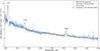 |
Fig. 2. Rest-frame spectrum of SDSS J101353 (blue) shown with the fitted continuum (orange) and the broadened iron emission (dashed violet). For comparison, composite quasar spectrum 2 from Richards et al. (2003) is also displayed (black). |
3.2. Mg II emission line fitting and black hole mass estimation
The masses of black holes (BHs) in AGNs can be estimated using several complementary techniques. The most direct approach is the reverberation mapping, which measures time delays between continuum and emission-line variations to infer the BLR size and, hence, the virial mass. When such monitoring data are unavailable, single-epoch methods based on broad-line widths and empirical scaling relations provide a reliable alternative. Therefore, we used the Mg II emission line (commonly referred to as Mg II λ 2800 Å) to determine the central BH mass of SDSS J101353. The Mg II feature is a resonance doublet at λ 2797 Å and λ 2803 Å. In broad-line AGNs, the typical line width (a few thousand km s−1) exceeds the separation of the two components (corresponding to a velocity difference of ∼770 km s−1), so they are blended and treated as a single feature near 2800 Å. This approximation is widely adopted in single-epoch virial mass estimators and has a negligible impact on the inferred BH mass. The line was fitted using a Gaussian profile, as shown in Fig. 3. The results of the fit are summarized in Table 2. We found a rest frame EW of 10.89 ± 0.57 Å. To verify the robustness of the derived line parameters, we tested whether the fit depends on the data binning. We found that the FWHM remains consistent within the fitting uncertainties for different binning methods, and therefore its value can be reliably used for the BH mass estimation. The monochromatic luminosity at 3000 Å taken from the SDSS spectrum of SDSS J101353 is λ Lλ (3000 Å) = 2.07 × 1045 erg s−1. This luminosity is typical for a quasar (Dempsey & Zakamska 2018). We used the bolometric correction at 3000 Å from Shen et al. (2011), BC3000 = 5.15 and obtained a bolometric luminosity of 1.06 × 1046 erg s−1. We calculated the mass of the BH (in units of solar mass M⊙) using Eq. (1) from Vestergaard & Osmer (2009):
![Mathematical equation: $$ \begin{aligned} {M}_{\text{BH}} = 10^{6.86} \left[ \frac{\text{ FWHM}(\text{ Mg} \text{ II})}{1000\ \text{ km/s}} \right]^2 \left[ \frac{\lambda L_{\lambda }(3000\,\AA )}{10^{44}\, \text{ erg/s}} \right]^{0.5}. \end{aligned} $$](/articles/aa/full_html/2026/04/aa58737-25/aa58737-25-eq1.gif)
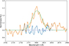 |
Fig. 3. Mg II emission line fitting. The re-binned rest-frame spectrum of SDSS J101353 after iron subtraction is displayed in orange. The underlying continuum is shown in blue. The dashed green line shows the best fit with a single Gaussian. |
Rest-frame Mg II properties of SDSS J101353.
We found a mass of (4.95 ± 0.64)×108 M⊙, consistent with those found in the literature, in particular with those from Vestergaard et al. (2008, their Fig. 1). Knowing the BH mass, we could determine the Eddington accretion rate using the relation: ṁ = Lbol/LEdd, where Lbol is the bolometric luminosity and LEdd is the Eddington luminosity (Rybicki & Lightman 1979). The accretion rate of our WLQ is 0.17. In the sample of about 300 type-1 quasars studied by Sulentic et al. (2006), quasars with similar redshifts have masses ranging from ∼6 × 10⁸ to ∼1010 M⊙ (see their Fig. 5) and show an accretion rate ranging from ∼0.15 to ∼1.20 (see their Fig. 7).
4. Disk fitting method
Another method of estimating the mass and the accretion rate of an accreting source is to model its broadband SED. Therefore, we fitted the broadband SED of SDSS J101353 using the X-ray Spectral fitting package XSPEC (version 12.13.1, Arnaud 1996). The optical-UV bump is attributed to the emission generated by the accretion disk surrounding the central engine. The X-ray data points are interpreted as emission from a Comptonizing reservoir, such as a hot corona and a warm region. A file containing additional optical-UV continuum photometric data, in addition to ugriz, was created from the SDSS spectrum file by selecting the continuum windows of Kuraszkiewicz et al. (2002) listed in Table 1. The SDSS spectrum was binned and converted into XSPEC compatible files. For this step, we used the tool ftflx2xsp. The generated SED file used in XSPEC contains 20 data points.
Corrections are necessary for the data because they are tainted by various factors. We explain these corrections first in the next subsection. The spectral analyses using XSPEC are detailed further below.
4.1. Data corrections
We corrected our observed data for Galactic reddening using the command redden. We used the color excess E(B − V) of 0.0081 ± 0.0009 mag that was previously determined for SDSS J101353 from the dust reddening map (Schlegel et al. 1998; Schlafly & Finkbeiner 2011).
We also applied a photoelectric absorption correction caused by the Galactic and intergalactic medium using the command phabs. This photoelectric absorption influences in particular the X-ray fluxes. We used the measurement of the Galactic neutral atomic hydrogen column density, NH, derived from the HI 4π all-sky survey (HI4PI Collaboration 2016), which is 9.15 × 1019 cm−2. In all the fitted models, the color excess, NH, the redshift and the distance of the quasar are fixed.
4.2. Starlight and torus contributions
Another factor to consider is the contribution of starlight to the SED from the stars of the galaxy hosting the quasar. It is often suggested that this contribution is negligible (Shen et al. 2011). However, we decided to include it. We tested different templates of Polletta et al. (2007). Assuming that the galaxies hosting quasars are elliptical, we used in particular the template of a 5 gigayear-old elliptical galaxy that matches our redshift. We created this component in the form of a readable XSPEC file due to the absence of such a model in this package. Adding a starlight component to our SED gives better fit results, especially for the IR data.
As the WISE data show evidence of a dusty torus surrounding the central engine and its accretion disk, we added one blackbody component to our SED (bbody model in XSPEC) as thermal emission from the torus. The mean temperature obtained is 930 ± 100 K. The typical hot thermal dust emission in WLQs ranges from 870 K to 1240 K according to Diamond-Stanic et al. (2009). This is close to the typical emission of host dust in type-1 quasars, ranging from 1100 K to 2200 K, according to Collinson et al. (2017).
4.3. Fitting using a multi-temperature blackbody model and a power law
We fitted the available photometric points with a minimal physical model consisting of a relativistic multicolor blackbody model using the kerrbb component (Li et al. 2005) in XSPEC to represent the accretion disk emission, along with a simple power-law component intended to model the X-ray emission (hereafter Model 1a, illustrated in Fig. 4).
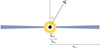 |
Fig. 4. Schematic geometry used in the fitting process for Model 1a. The BH is in black, the standard geometrically thin accretion disk in blue-gray, and the hot corona in yellow. |
All additive components of Model 1a are corrected for the quasar’s redshift. This model is described as follows:
 (1)
(1)
The relativistic model kerrbb describes the emission of a thin disk around a BH described by a Kerr metric. The key assumption of the kerrbb model is that all the heat generated within the accretion disk is instantaneously radiated away, with no significant energy advection or internal storage. This model was originally developed to describe the thermal emission from accretion disks around stellar-mass BHs, particularly in X-ray binaries. However, in our study, we extended its application to supermassive BHs.
The starlight and bbody components represent the starlight contribution from the host galaxy and the dusty torus, respectively (as explained in the previous subsection). Since supermassive BHs in the centers of quasars are expected to possess nonzero spin, we tested whether our data can constrain the spin of SDSS J101353. To do this, we generated χ2 confidence contours in the spin-inclination plane, allowing the BH mass and the mass accretion rate to vary freely. The confidence contours (Fig. 5) indicate a mild preference for high-spin values. A nonrotating BH remains allowed at the 99% confidence level. The inclination is best constrained around 50°, with a 68% confidence range of approximately 45°–60°. We also examined how the inferred BH mass and accretion rate depend on the assumed spin value. The results are shown in Fig. 6. Overall, the spin remains unconstrained. Adopting a zero-spin configuration therefore provides a reasonable baseline for the disk modeling. We fixed the torque parameter (defined as the ratio of the disk power produced by a torque at the disk inner boundary to the disk power arising from accretion) to zero, corresponding to a standard Keplerian disk configuration around a nonrotating BH. We assumed a disk’s inclination angle (that is, the angle between the axis of the disk and the line of sight) to 30°, consistent with the properties of type-1 quasars. However, we tested it, modifying the inclination angle gives results that remain in a reasonable range, as shown in Table 3. We decided to keep the value of 30° as a reference value for the next more sophisticated models.
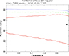 |
Fig. 5. χ2 confidence contours in the spin-inclination (a–i) plane determined using Model 1a: kerrbb + power-law components. They were obtained by allowing the BH mass and mass accretion rate to vary. The solid red, dashed green, and dotted blue contours correspond to the 68%, 90%, and 99% confidence levels, respectively. The cross indicates the best-fit solution. |
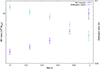 |
Fig. 6. Dependence of the inferred BH mass and Eddington ratio on the adopted spin parameter, a, calculated for Model 1a, with an inclination i = 50°. |
kerrbb parameter results for different values of the inclination angle, i.
The best-fit parameters are summarized in Table 4 and the broadband SED fit is shown in Fig. 7. The fit quality (χ2/d.o.f. = 10.31/13) indicates that this simple model is sufficient to describe the data within the observational uncertainties. The fundamental parameters, BH mass and Eddington accretion rate, are typical to normal quasars (Shen et al. 2011). The results show that the source emission in hard X-rays is very weak, ≈10−5 of the total luminosity. The fitted photon index, Γ = 1.8 ± 0.8, is consistent with typical AGN values (Γ ≈ 1.7 − 2.5). This suggests either an intrinsically weak hot corona or the presence of a partial obscuration (i.e., shielding) of the corona such that only reflected X-rays reach the observer.
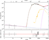 |
Fig. 7. Broadband SED fit of SDSS J101353 using Model 1a: kerrbb + power-law components. Top panel: Best-fit model (solid red line) to the data (black dots). The dashed green and blue lines represent kerrbb and power-law components, respectively. The starlight and torus contributions are shown in yellow and violet, respectively. Bottom panel: Residuals of χ2 related to the total model. |
Fitting results for SDSS J101353 using different models and assuming an inclination angle of 30° from the accretion disk axis.
We performed a stepping investigation on the BH mass (parameter Mbh) and the mass accretion rate of the disk (parameter Mdd) to test the robustness of the fit and to explore possible parameter degeneracies. Figure 8 displays the χ2 confidence contours between the BH mass and the mass accretion rate obtained from this analysis. The red, green, and blue contours correspond to the 68%, 90%, and 99% confidence levels, respectively. The elongated shape of the contours reveals a degeneracy between the two parameters: larger BH masses require lower accretion rates to reproduce the same continuum shape. This trend reflects the intrinsic coupling between these parameters in thin-disk models, as both govern the disk temperature distribution and normalization. The best-fit solution (black cross) corresponds to Mbh ≈ 2 × 10⁹ M⊙ and Mdd ≈ 6.5 M⊙ yr−1. These values imply an Eddington ratio (ṁ ≈ 0.087) consistent with a moderately accreting quasar, supporting the physical plausibility of the fit within the standard thin-disk framework.
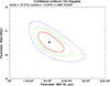 |
Fig. 8. Confidence contours for the BH mass and the mass accretion rate for Model 1a. The solid red, dashed green, and dotted blue contours correspond to the 68%, 90%, and 99% confidence levels, respectively. The cross marks the best-fit values. |
The Eddington accretion rates inferred from the single-epoch method (Sect. 3.2) and from the SED fitting differ by some factor. Such differences are expected, as single-epoch virial estimates rely on broad-line widths and are therefore sensitive to uncertainties in the BLR geometry and dynamics, whereas the SED-based method provides a BLR-independent estimate of the accretion flow. In particular, the FWHM measured from single-epoch spectra may be affected in WLQs, leading to biased virial mass and accretion rate estimates (e.g., Mejía-Restrepo et al. 2018; Marculewicz & Nikolajuk 2020).
4.4. Fitting using an AGN SED model
While kerrbb provides a relativistic model of the disk emission around a BH, assuming local energy dissipation and purely thermal radiation, it does not include other important emission components known to shape AGNs continua, such as Comptonization in warm and hot corona. To model these features, we adopted the model relagn (Hagen & Done 2023), a relativistic extension of the agnsed framework (Kubota & Done 2018). relagn retains the physical three-zone structure of agnsed – a standard outer disk, a warm Comptonizing region responsible for the soft excess, and a hot corona producing the X-ray power law – while incorporating full relativistic effects on the disk emission. In both agnsed and relagn, all radiative power originates from gravitational energy released in the accretion disk. A fraction of this energy is locally diverted to power the warm and hot Comptonizing regions, while the remainder is emitted as thermal disk radiation. Thus, the warm and hot coronae do not constitute independent energy sources but reprocess disk dissipation within their respective radial zones. This makes relagn a more appropriate model for modeling the full broadband SED of quasars.
The strength of both the hot and warm coronae are parameterized by their outer radius, Rhot and Rwarm, respectively, with their minimum values at the innermost stable circular orbit (ISCO) indicating no corona at all. In all the fits performed, we fixed the outer radius of the accretion disk Rout to 105Rg, the upper limit of the scale height for the hot component to the default value, 10 Rg, and we did not consider reprocessing mechanisms. We assumed a non-spinning BH, so ISCO is at 6 Rg. As previously, we fixed the inclination angle (between the axis of the disk and the line of sight) to 30°.
We fitted the broadband SED of SDSS J101353, focusing on the possible contribution of a hot corona and a warm region. For that, we tested two configurations with the following model:
 (2)
(2)
We first attempted to fit Rhot, meaning the strength of the hot corona, assuming no warm corona, Rwarm fixed at 6 Rg. The best fit was obtained for Rhot = 6Rg, meaning no hot corona at all, even though the data show the weak X-ray emission. We conclude that this result is obtained because, due to numerical reasons, the relagn model is not able to reproduce such a weak hot corona. Therefore, in the following we simply fix Rhot at 6 Rg and add the weak power law4 with fixed index of 1.8 to describe the X-ray data points. Letting the multicolor disk component of the relagn model to reproduce the optical-UV emission, the fit yields, with acceptable statistics, a slightly lower BH mass of 1.51 × 10⁹ M⊙, but this solution stresses the disk energetics, leading to a higher accretion rate ṁ of 0.174, and does not naturally produce the soft X-ray excess. This is our Model 1b. The fitting parameters are shown in Table 4 and the corresponding best fit is displayed in Fig. 9a. The plot includes the separate power-law component modeling the X-ray data points.
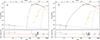 |
Fig. 9. Broadband SED fit of SDSS J101353 using relagn model. Panel (a): Accretion disk with a very weak and compact hot corona configuration (Model 1b). Panel (b): Same configuration as in (a) but leaving the warm region parameters free (Model 2). Top subpanels: Best-fit model (solid red line) to the data (black dots). The dashed green line represents the relagn component. The starlight and torus contributions are shown in yellow and violet, respectively. An artificial power law (dotted blue line) is displayed to show the contribution of a compact weak hot corona. Bottom subpanels: Residuals of χ2 related to the total model in red (without taking the artificial power law into account). |
Secondly, we focused on the warm region. Although the results of the previous fit formally indicate that a warm region contribution is not required by the data (χ2 < 1), we decided to test for the presence of a warm corona. The motivation comes from the fact that the spectral component attributed to a warm corona is quite often observed in spectra of high accretion rate AGN and X-ray binaries (Done et al. 2007; Petrucci et al. 2018). This is our Model 2, illustrated in Fig. 10.
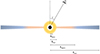 |
Fig. 10. Schematic geometry used in the fitting process for Model 2. As in Fig. 4, the BH is in black, the standard accretion disk in blue-gray, and the compact and weak hot corona in yellow. The warm region is in light orange. |
Allowing for a warm corona in the relagn model considerably improves the fit, with Δχ2 = 8.69 for three fewer degrees of freedom. The best-fit warm region has  ,
,  , and
, and  , consistent with an optically thick warm corona extending to tens of gravitational radii and invoked to produce the soft X-ray – UV excess. The best-fit results are reported in Table 4 and plotted in Fig. 9b. So, Model 2 provides a significantly improved fit, although we do note that the improvement mainly comes from the two highest energy points in UV, around 1000 Å, and there are no data points in FUV – soft X-ray range where this spectral component would be directly observable. To evaluate the influence of the 10-keV X-ray data point, we also performed a fit excluding it: the fit quality improved from χ2 = 3.93 for 12 d.o.f. to χ2 = 2.37 for 11 d.o.f., as expected when removing the highest-energy constrain.
5. The obscuration scenario and X-ray reflection
The low level of X-ray emission in SDSS J101353 can a priori be explained in two ways. Firstly, it can be a very weak intrinsic emission from the central X-ray source, similar to spectral states observed in some soft X-ray transients. This spectral state is referred to as the ultrasoft state (USS) and occurs at an accretion rate not too high above the transition from hard state to soft state (see, e.g., Done et al. 2007 for a review).
The second possibility is to assume that the central X-ray source is obscured and only a reflected component is reaching the distant observer; we refer to this as Model 3 (see Fig. 11). This scenario, which is compatible with general ideas about a broad range of X-ray emission in WLQs (Cheng et al. 2025), assumes that the obscuration, which is generally invoked to reduce the high-energy radiation reaching the BLR and to explain the WLQ phenomenon, can also affect the emission directed toward the observer. Thus, the observed emission corresponds only to the reprocessed component while the intrinsic X-ray level is noticeably higher.
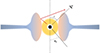 |
Fig. 11. Schematic illustration of the obscuration scenario (Model 3) showing the reflected emission received by an observer with an inclination angle i = 45°. The central BH and the hot corona are depicted as in Fig. 10. The gaseous obscurer is represented by the puffed-up shape and has an opening angle θ0. |
This scenario would require that the obscurer is, for example, geometrically extended to the lines of sight toward an observer and its optical depth is high enough to completely block the X-rays that, when redshifted to the observer’s frame, would have been observed in the typical energy band of our X-ray detectors, E > 0.1 keV. We attempted to estimate the level of intrinsic emission in this scenario. We used a Monte Carlo code for radiative transfer in optically thick media that had previously been done in the context of obscuration in Seyfert 2 galaxies (e.g., Madejski et al. 2000).
We considered a simple torus geometry with a rectangular cross section, parameterized by its vertical and radial Thomson depth and by its half-opening angle. By assumption, the torus is Thomson very thick along the line of sight to the observer. Considering that quasars are expected to be viewed at low to moderate inclination angle, the opening angle cannot be too large. In our baseline case, the torus has a half-opening angle of 20° and a square cross section with τT = 10.
Monte Carlo simulations of photons isotropically emitted at the center of the system and transferred through this medium include the processes of photoelectric absorption and Compton scattering. The implemented atomic data allow for simulations of the fluorescent Fe Kα line photons to be considered in the case of non-ionized plasma. We investigated two limiting scenarios: (i) a neutral torus with solar elemental abundances, and (ii) a pure-scattering case with no photoelectric absorption, as might approximate a hot, puffed-up inner disk obscuring structure (but note that we do not consider Compton up-scattering in this case).
The results presented in Fig. 12 show unfolded spectra where FE is the energy flux density per unit energy. The spectrum is shown as EFE to illustrate the energy at which the broadband SED peak occurs. The spectra indicate that the reflected hard X-ray spectrum is not significantly suppressed compared to the intrinsic emission. At ∼30 keV, the ratio of primary to reflected flux is not higher than 4 for viewing angles of ∼40° (see the magenta histogram). Having estimated the primary emission in this way, we could then construct the spectrum reaching the BLR, i.e., the intrinsic spectrum. For this, we modeled the data replacing the power law with the pexrav model (representing the reflected component; see Magdziarz & Zdziarski 1995), and using the nthcomp model to represent a thermally Comptonized continuum (Zdziarski et al. 1996; Życki et al. 1999), to fit to the hard X-ray points, and then adjust the amplitude of the required primary emission so that the ratio of fluxes at 10 keV (approximately 30 keV redshifted to the observer frame) is equal to 4. nthcomp thus provides the primary continuum emission. This is represented in Fig. 13, where the resulting spectrum is plotted. The results of our spectrum inspection and our SED fitting highlight both the extreme X-ray weakness and the lack of prominent emission lines in SDSS J101353, raising important questions about the physical processes at play. In the following discussion, we consider several possible scenarios that could explain these peculiar properties.
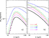 |
Fig. 12. Spectra of the component reflected by the toroidal material obscuring the central source. Panel (a): Case of cold, non-ionized plasma. Panel (b): Fully ionized case (but note that Compton up-scattering is not taken into account). The thin black line is the primary emission (we assumed a thermal Comptonization of kTe = 100 keV), the thick black line shows the angle-averaged reflected component, and the colored lines show the dependence of the reflected spectra on the viewing angle, i, for i < 50°. |
 |
Fig. 13. Broadband SED fit of SDSS J101353 with the primary emission (dashed blue curve) estimated using pexrav and nthcomp in Model 3. As previously, the solid red line represents the total model. The relagn component and the starlight and torus contributions are shown in green, yellow, and violet, respectively. The data are displayed with the black dots. |
6. Discussion
The WLQ SDSS J101353 combines two properties that place it among the most extreme WLQs: a nearly featureless UV-optical spectrum, with only a weak Mg II emission line (while both C III] and C IV are almost absent), and a pronounced X-ray weakness, ∼4 orders of magnitude below expectations for normal quasars. This dual deficit challenges standard quasar models and requires considering both accretion physics and BLR conditions. The quasi-absence of high-ionization emission lines may result from a combination of factors: a sparsely populated BLR, shielding of ionizing photons, or a fundamentally different X-ray SED (Shemmer et al. 2009; Luo et al. 2015). Nevertheless, in this article, we do not consider the production of emission lines by the BLR or the presence of the BLR itself. Our analysis focuses exclusively on the continuum emission. More precisely, our fitting constrains the thermal emission from the accretion disk, the presence of a parsec-scale torus, and the starlight from the host galaxy. These components alone, however, cannot account for the suppression of the emission lines.
We confirm that the shape of the IR/optical continuum of SDSS J101353 is standard, lying within the range of shapes observed in other type-1 quasars (the photon index of our WLQ αν = −0.46). However, the low level of X-ray radiation is puzzling. There are two possible explanations. The first is that the central X-ray emitter is intrinsically faint. The second is that the weak signal results from heavy obscuration of the primary X-ray source.
Investigating the first scenario, we modeled the continuum of SDSS J101353 using both kerrbb and relagn models (in XSPEC), which provided an independent and physically motivated estimate of the accretion flow. The best fits of both models suggest that the thermal emission extends down to the ISCO, consistent with a standard thin disk. A disk-dominated configuration with an exceptionally weak hot corona (which is inefficient, very compact, or partially quenched) is therefore favored. The hot corona can only generate a very small amount of energy, to account for the observed X-ray data. Nevertheless, the inferred coronal parameters themselves are comparable to those reported for typical quasars. Its photon index Γ = 1.8.
The weak emission lines observed in SDSS J101353 are difficult to interpret. Laor & Davis (2011) proposed that an inefficient cold accretion disk caused by a very massive BH could generate a non-ionizing continuum. In their model, the accretion disk becomes too cold to ionize when MBH > 3.6 × 10⁹ M⊙ for a nonrotating BH. This threshold is derived under the assumptions that the typical X-ray luminosity observed in quasars satisfies LX ≲ Lbol and that the ionizing luminosity of a cold accretion disk is only Lion ∼ 0.01 Lbol (where Lbol is the bolometric luminosity). For SDSS J101353, in the case of Models 1a/1b, we got log(LX/Lbol) = − 4.87 and Lion/Lbol ≃ 0.002, and the supermassive BH may be lighter than the aforementioned upper limit. From the single-epoch Mg II line, we found a BH mass of ∼5 × 10⁸ M⊙, typical of normal quasars. Nevertheless, these estimates are subject to biases affecting WLQs. Marculewicz & Nikolajuk (2020) show that virial masses derived from the FWHM of Hβ can be underestimated by factors of 4-5 in WLQs, compared with disk-fitting techniques, due to geometric or dynamical differences in their BLRs. If a similar bias affects the Mg II line, then the true mass of SDSS J101353 may be significantly higher than the single-epoch estimate. Indeed, our continuum modeling using the disk-fitting methods (both kerrbb and relagn models) provides a physically motivated, BLR-geometry-independent estimate of the accretion flow. The two methods converge toward a higher BH mass of ∼(1.5 − 2.1)×109 M⊙, but this is still lower than the upper limit found by Laor & Davis (2011).
The inclusion, in our relagn fit (i.e., Model 2), of a warm, optically thick Comptonizing region substantially improves the fit. From this warm-corona fit (kTe ≈ 0.20 keV, Γ ≈ 3.80) and using the definition of Γ in Beloborodov et al. (1999), we found that the warm corona has an optical depth of τ ≈ 7.26. The presence of a warm Comptonizing region supports a configuration seen in many AGNs (e.g., Kubota & Done 2018; Petrucci et al. 2018; Middei et al. 2020), although the limited X-ray data prevent us from placing strong constraints. These works show that such warm Comptonizing layers are a robust explanation for the soft X-ray excess and line production in quasars. Our results suggest that SDSS J101353 shares similar physical conditions with them, despite its extreme weakness in the hard X-ray band. In Model 2, we obtained log(LX/Lbol) = − 4.29 and Lion/Lbol ≃ 0.05, both of which are still low.
This suggests that the X-ray level and the reduced coronal contribution are intrinsic, indicating that the corona is either physically absent or unusually compact. The quasar continuum resembles the spectral behavior observed in certain soft X-ray transients – a subclass of X-ray binaries. These transients typically appear when the accretion rate is only slightly above the threshold that separates the hard and soft states. As shown by Done et al. (2007), the transitions from the hard state to the USS are accompanied by dramatic changes in the geometry of the inner accretion flow, particularly a strong suppression or disappearance of the hot Comptonizing corona (see their Fig. 9). In the USS, the spectrum becomes almost entirely disk-dominated, with only a faint high-energy tail. This configuration closely resembles the SED of SDSS J101353. If this analogy holds, then this WLQ may represent an AGN version of a low-corona state, naturally suppressing the production of high-energy photons and the ionizing continuum required to power high-ionization emission lines. This provides a unified explanation for the simultaneous weakness of emission lines and the X-ray deficit.
Regarding the X-ray weakness, we propose a second explanation for this phenomenon seen in SDSS J101353. While the USS analogy offers a compelling physical picture, geometric effects may also contribute. The production of a shielding gas or a puffed-up inner disk between the inner region and the observer (Model 3) means that the observer only detects radiation that has been reflected or reprocessed. The X-ray level is lower than typical and the shielding gas attenuates the ionizing continuum reached by HILs while still allowing the outer BLR to receive some radiation by LILs (e.g., Wu et al. 2011; Gallo et al. 2011; Cheng et al. 2025). Our SED fits cannot rule out such a configuration. Therefore, we tested a reflection-dominated X-ray flux that could mimic the observed faintness. The resulting estimated primary X-ray flux is still 102–103 times fainter than that of a typical quasar. The explanation for the emergence of the puffed-up inner disk is the slim disk solution (Abramowicz et al. 1988; Czerny 2019). It requires a high accretion rate (sub- or super-Eddington). From the single-epoch Mg II line, we found an Eddington accretion rate of 0.17, typical of normal quasars. The corresponding accretion rate is modest compared to the range values of 0.3–0.6 reported for WLQ samples (Marculewicz & Nikolajuk 2020). In contrast, Cheng et al. (2025) argue that WLQ accretion rates may be underestimated in single-epoch methods, especially when the EW of C IV decreases. Notably, their figure 12 shows that the Eddington ratio distribution of WLQs (at redshifts from 1.45 to 1.90) is not dramatically higher than for normal quasars. Their calculated mean Eddington ratios are ṁ = 0.151 for WLQs, and ṁ = 0.119 for normal quasars. This indicates that the high-Eddington WLQ picture may not apply uniformly across all redshifts and all WLQ subclasses. Our result for SDSS J101353 fits naturally into this more nuanced view. Additionally, our continuum modeling using XSPEC models for the disk fitting provides a still moderate Eddington accretion rate ṁ ∼ 0.1 in this WLQ. This may suggest a greater likelihood of SDSS J101353 being in the USS state than of the presence of the shielding gas or puffed-up inner accretion disk.
According to the Mg II emission line fit, we know that the FWHM of this line is 3875 ± 250 km s−1. In addition, its UV iron-to-magnesium ratio RFeII, UV, defined as EW(Fe IIUV(λ2700−2900Å))/EW(Mg II)}, lies in the range 5.5–7.9. These values were derived using the relations between FWHM(MgII),EW(MgII) and EW(FeIIUV) for quasars (Śniegowska et al. 2020). It is worth mentioning that these values classify our WLQ as a member of the A population of the quasar main sequence. Sources belonging to this population are characterized by higher accretion rates (e.g., log ṁ ≳ −1.3 in Marziani’s sample), narrower lines, a higher intensity Fe II to Mg II ratio, blueshifted C IV, and the presence of a strong wind (Marziani et al. 2024).
All our conclusions are further confirmed by the value of the so-called X-ray loudness, i.e., the αOX parameter (Sobolewska et al. 2009), which represents the ratio of optical to X-ray luminosity weighted by the wavelength for which both luminosities have been calculated. In the case of the data collected of our special quasar, and for two energy points 2500 Å and 2 keV5, we obtained αOX = 2.06. Together with the derived Eddington accretion rate, it puts SDSS J101353 in the top-right corner of the αOX versus ṁ plane for quasars presented by Ruan et al. (2019, see their Fig. 3). This finding fully confirms conclusions of this paper that the source is in its high (soft) spectral state, where the corona is confined to the compact inner hot region.
The weak corona might also be episodic. Indeed, another possibility is that SDSS J101353 is undergoing a changing-look, or state-change phase. A reduced coupling between the disk and corona could lead to a transient phase characterized by diminished X-ray emission and suppressed HILs. Such a behavior has been reported in nearby AGNs, where quasars have transitioned from X-ray-bright to X-ray-weak states, sometimes accompanied by spectral changes in the BLR (e.g., Noda & Done 2018; Ruan et al. 2019). If SDSS J101353 is caught during such a weak-corona state, this could simultaneously explain its current X-ray faintness and line suppression. Recent observations of a “reawakening” in the AGN Markarian 590 (Palit et al. 2025) show that a rising continuum, including a reemerging warm corona and increased soft X-ray/UV flux, is accompanied by the return of broad Balmer lines and HILs.
7. Conclusions
We performed a detailed broadband spectral analysis of the WLQ SDSS J101353, a quasar with two remarkable features: a nearly featureless optical-UV continuum, with only a faint Mg II line clearly detected, and exceptionally weak X-ray emission. We have focused on its continuum and X-ray properties. Our main conclusions are summarized as follows:
-
Robust continuum fitting: The relativistic thin-disk model kerrbb combined with a power law and the multicomponent relagn model yields consistent BH parameters (MBH ∼ 2 × 10⁹ M⊙, ṁ ∼ 0.1), confirming that SDSS J101353 accretes at a typical quasar rate. However, the coronal emission is markedly suppressed.
-
Evidence of a warm corona: Including a warm, optically thick Comptonizing region (kTe, warm ≈ 0.20 keV, Γwarm ≈ 3.8, and Rwarm extended to 34 Rg) significantly improves the fit, pointing toward an inefficient or compact corona as the primary cause of the X-ray faintness.
-
Additional mechanisms: We investigated additional physical mechanisms, such as shielding by a thick inner disk and a partial absorption of ionizing photons. If we assume that we only see the X-ray emission reflected by the shielding gas, the primary X-ray level remains low, no more than 4 times the observed one. This indicates the intrinsic weakness of the hot corona.
-
Implications for WLQ diversity: SDSS J101353 reinforces the view that WLQs constitute a heterogeneous population in which both structural and temporal effects can suppress the production of high-energy photons and broad emission lines. This source may represent an AGN version of the ultrasoft state (USS) seen in some soft X-ray transients. This spectral state occurs in X-ray binaries at an accretion rate not too high above the transition from the hard state to the soft state.
Taken together, our results suggest that SDSS J101353 offers a valuable counterexample to the idea that all WLQs are extreme high-Eddington accretors.
Future work (Paper II) will explore detailed photoionization simulations using Cloudy, testing whether the observed emission line weakness can be reproduced under different continuum and geometry assumptions. Multi-epoch observations could also be essential for determining whether the X-ray weakness of SDSS J101353 reflects a stable configuration or a transient state of the accretion flow.
Acknowledgments
The authors thank Marianne Vestergaard for providing the iron emission template, and Profs. Czerny and Done for helpful discussions and advice. They also thank the anonymous referee for constructive comments that improved the manuscript. The research leading to these results has received funding from the European Union’s Horizon 2020 Programme under the AHEAD2020 project (grant agreement n. 871158). RW has been fully and AR has been partially supported by the Polish National Science Center grant No. 2021/41/B/ST9/04110.
References
- Abdurro’uf, Accetta, K., Aerts, C., et al. 2022, ApJS, 259, 35 [NASA ADS] [CrossRef] [Google Scholar]
- Abramowicz, M. A., Czerny, B., Lasota, J. P., & Szuszkiewicz, E. 1988, ApJ, 332, 646 [Google Scholar]
- Andika, I. T., Jahnke, K., Onoue, M., et al. 2020, ApJ, 903, 34 [Google Scholar]
- Arnaud, K. A. 1996, in Astronomical Data Analysis Software and Systems V, eds. G. H. Jacoby, & J. Barnes, ASP Conf. Ser., 101, 17 [NASA ADS] [Google Scholar]
- Beloborodov, A. M. 1999, in High Energy Processes in Accreting Black Holes, eds. J. Poutanen, & R. Svensson, ASP Conf. Ser., 161, 295 [Google Scholar]
- Bianchi, L., Herald, J., Efremova, B., et al. 2011, Ap&SS, 335, 161 [Google Scholar]
- Boller, T., Freyberg, M. J., Trümper, J., et al. 2016, A&A, 588, A103 [NASA ADS] [CrossRef] [EDP Sciences] [Google Scholar]
- Cardelli, J. A., Clayton, G. C., & Mathis, J. S. 1989, ApJ, 345, 245 [Google Scholar]
- Cheng, X., Wu, J., & Wu, Q. 2025, arXiv e-prints [arXiv:2510.08135] [Google Scholar]
- Collinson, J. S., Ward, M. J., Landt, H., et al. 2017, MNRAS, 465, 358 [NASA ADS] [CrossRef] [Google Scholar]
- Collin-Souffrin, S., & Lasota, J.-P. 1988, PASP, 100, 1041 [NASA ADS] [CrossRef] [Google Scholar]
- Czerny, B. 2019, Universe, 5, 131 [NASA ADS] [CrossRef] [Google Scholar]
- Dempsey, R., & Zakamska, N. L. 2018, MNRAS, 477, 4615 [NASA ADS] [CrossRef] [Google Scholar]
- Diamond-Stanic, A. M., Fan, X., Brandt, W. N., et al. 2009, ApJ, 699, 782 [NASA ADS] [CrossRef] [Google Scholar]
- Done, C., Gierliński, M., & Kubota, A. 2007, A&A Rev., 15, 1 [CrossRef] [Google Scholar]
- Evans, I. N., Primini, F. A., Glotfelty, K. J., et al. 2010, ApJS, 189, 37 [NASA ADS] [CrossRef] [Google Scholar]
- Fitzpatrick, E. L. 1999, PASP, 111, 63 [Google Scholar]
- Gallo, L. C., Grupe, D., Schartel, N., et al. 2011, MNRAS, 412, 161 [NASA ADS] [CrossRef] [Google Scholar]
- Gaskell, C. M., Goosmann, R. W., Antonucci, R. R. J., & Whysong, D. H. 2004, ApJ, 616, 147 [NASA ADS] [CrossRef] [Google Scholar]
- Hagen, S., & Done, C. 2023, MNRAS, 525, 3455 [NASA ADS] [CrossRef] [Google Scholar]
- HI4PI Collaboration (Ben Bekhti, N., et al.) 2016, A&A, 594, A116 [NASA ADS] [CrossRef] [EDP Sciences] [Google Scholar]
- Hryniewicz, K., Czerny, B., Nikołajuk, M., & Kuraszkiewicz, J. 2010, MNRAS, 404, 2028 [NASA ADS] [Google Scholar]
- Kubota, A., & Done, C. 2018, MNRAS, 480, 1247 [Google Scholar]
- Kuraszkiewicz, J. K., Green, P. J., Forster, K., et al. 2002, ApJS, 143, 257 [NASA ADS] [CrossRef] [Google Scholar]
- Laor, A., & Davis, S. W. 2011, MNRAS, 417, 681 [NASA ADS] [CrossRef] [Google Scholar]
- Leighly, K. M., Halpern, J. P., Jenkins, E. B., et al. 2007, ApJ, 663, 103 [Google Scholar]
- Li, L.-X., Zimmerman, E. R., Narayan, R., & McClintock, J. E. 2005, ApJS, 157, 335 [NASA ADS] [CrossRef] [Google Scholar]
- Luo, B., Brandt, W. N., Hall, P. B., et al. 2015, ApJ, 805, 122 [Google Scholar]
- Madejski, G., Życki, P., Done, C., et al. 2000, ApJ, 535, L87 [NASA ADS] [CrossRef] [Google Scholar]
- Magdziarz, P., & Zdziarski, A. A. 1995, MNRAS, 273, 837 [Google Scholar]
- Marculewicz, M., & Nikolajuk, M. 2020, ApJ, 897, 117 [NASA ADS] [CrossRef] [Google Scholar]
- Marziani, P., Floris, A., Deconto-Machado, A., et al. 2024, Physics, 6, 216 [NASA ADS] [CrossRef] [Google Scholar]
- McDowell, J. C., Canizares, C., Elvis, M., et al. 1995, ApJ, 450, 585 [NASA ADS] [CrossRef] [Google Scholar]
- Mejía-Restrepo, J. E., Lira, P., Netzer, H., Trakhtenbrot, B., & Capellupo, D. M. 2018, Nat. Astron., 2, 63 [CrossRef] [Google Scholar]
- Middei, R., Petrucci, P. O., Bianchi, S., et al. 2020, A&A, 640, A99 [NASA ADS] [CrossRef] [EDP Sciences] [Google Scholar]
- Ni, Q., Brandt, W. N., Luo, B., et al. 2018, MNRAS, 480, 5184 [NASA ADS] [Google Scholar]
- Nikołajuk, M., & Walter, R. 2012, MNRAS, 420, 2518 [CrossRef] [Google Scholar]
- Noda, H., & Done, C. 2018, MNRAS, 480, 3898 [Google Scholar]
- Palit, B., Śniegowska, M., Markowitz, A., et al. 2025, MNRAS, 540, L14 [Google Scholar]
- Petrucci, P. O., Ursini, F., De Rosa, A., et al. 2018, A&A, 611, A59 [NASA ADS] [CrossRef] [EDP Sciences] [Google Scholar]
- Plotkin, R. M., Anderson, S. F., Brandt, W. N., et al. 2010, ApJ, 721, 562 [NASA ADS] [CrossRef] [Google Scholar]
- Polletta, M., Tajer, M., Maraschi, L., et al. 2007, ApJ, 663, 81 [NASA ADS] [CrossRef] [Google Scholar]
- Richards, G. T., Hall, P. B., Vanden Berk, D. E., et al. 2003, AJ, 126, 1131 [Google Scholar]
- Ruan, J. J., Anderson, S. F., Eracleous, M., et al. 2019, ApJ, 883, 76 [NASA ADS] [CrossRef] [Google Scholar]
- Rybicki, G. B., & Lightman, A. P. 1979, Radiative Processes in Astrophysics (New York: Wiley) [Google Scholar]
- Schlafly, E. F., & Finkbeiner, D. P. 2011, ApJ, 737, 103 [Google Scholar]
- Schlegel, D. J., Finkbeiner, D. P., & Davis, M. 1998, ApJ, 500, 525 [Google Scholar]
- Shemmer, O., Brandt, W. N., Anderson, S. F., et al. 2009, ApJ, 696, 580 [NASA ADS] [CrossRef] [Google Scholar]
- Shemmer, O., Trakhtenbrot, B., Anderson, S. F., et al. 2010, ApJ, 722, L152 [NASA ADS] [CrossRef] [Google Scholar]
- Shen, Y., Richards, G. T., Strauss, M. A., et al. 2011, ApJS, 194, 45 [Google Scholar]
- Śniegowska, M., Kozłowski, S., Czerny, B., Panda, S., & Hryniewicz, K. 2020, ApJ, 900, 64 [CrossRef] [Google Scholar]
- Sobolewska, M. A., Gierliński, M., & Siemiginowska, A. 2009, MNRAS, 394, 1640 [Google Scholar]
- Sulentic, J. W., Repetto, P., Stirpe, G. M., et al. 2006, A&A, 456, 929 [NASA ADS] [CrossRef] [EDP Sciences] [Google Scholar]
- Vestergaard, M., & Osmer, P. S. 2009, ApJ, 699, 800 [Google Scholar]
- Vestergaard, M., & Wilkes, B. J. 2001, ApJS, 134, 1 [Google Scholar]
- Vestergaard, M., Fan, X., Tremonti, C. A., Osmer, P. S., & Richards, G. T. 2008, ApJ, 674, L1 [NASA ADS] [CrossRef] [Google Scholar]
- Wills, B. J., Netzer, H., & Wills, D. 1985, ApJ, 288, 94 [NASA ADS] [CrossRef] [Google Scholar]
- Wright, E. L. 2006, PASP, 118, 1711 [NASA ADS] [CrossRef] [Google Scholar]
- Wright, E. L., Eisenhardt, P. R. M., Mainzer, A. K., et al. 2010, AJ, 140, 1868 [Google Scholar]
- Wu, J., Brandt, W. N., Hall, P. B., et al. 2011, ApJ, 736, 28 [NASA ADS] [CrossRef] [Google Scholar]
- Young, M., Elvis, M., & Risaliti, G. 2009, ApJS, 183, 17 [NASA ADS] [CrossRef] [Google Scholar]
- Zdziarski, A. A., Johnson, W. N., & Magdziarz, P. 1996, MNRAS, 283, 193 [NASA ADS] [CrossRef] [Google Scholar]
- Życki, P. T., Done, C., & Smith, D. A. 1999, MNRAS, 309, 561 [Google Scholar]
In XSPEC, the power law is defined in energy space as a photon spectrum NE ∝ E−Γ, where NE is the photon flux density (photons/keV/cm2/s), E is the photon energy (keV), and Γ is the photon index.
αOX = −0.3838 log [L(2 keV)/L(2500 Å)]. We use the minus sign; therefore, our αOX parameter is positive.
All Tables
Fitting results for SDSS J101353 using different models and assuming an inclination angle of 30° from the accretion disk axis.
All Figures
|
Fig. 1. Data points (black) and spectrum (blue; extracted from SDSS DR17) of SDSS J101353 in the observed frame. The light gray box represents the typical X-ray flux measured in the 2–10 keV energy band of classical quasars (e.g., Young et al. 2009). |
| In the text | |
|
Fig. 2. Rest-frame spectrum of SDSS J101353 (blue) shown with the fitted continuum (orange) and the broadened iron emission (dashed violet). For comparison, composite quasar spectrum 2 from Richards et al. (2003) is also displayed (black). |
| In the text | |
|
Fig. 3. Mg II emission line fitting. The re-binned rest-frame spectrum of SDSS J101353 after iron subtraction is displayed in orange. The underlying continuum is shown in blue. The dashed green line shows the best fit with a single Gaussian. |
| In the text | |
|
Fig. 4. Schematic geometry used in the fitting process for Model 1a. The BH is in black, the standard geometrically thin accretion disk in blue-gray, and the hot corona in yellow. |
| In the text | |
|
Fig. 5. χ2 confidence contours in the spin-inclination (a–i) plane determined using Model 1a: kerrbb + power-law components. They were obtained by allowing the BH mass and mass accretion rate to vary. The solid red, dashed green, and dotted blue contours correspond to the 68%, 90%, and 99% confidence levels, respectively. The cross indicates the best-fit solution. |
| In the text | |
|
Fig. 6. Dependence of the inferred BH mass and Eddington ratio on the adopted spin parameter, a, calculated for Model 1a, with an inclination i = 50°. |
| In the text | |
|
Fig. 7. Broadband SED fit of SDSS J101353 using Model 1a: kerrbb + power-law components. Top panel: Best-fit model (solid red line) to the data (black dots). The dashed green and blue lines represent kerrbb and power-law components, respectively. The starlight and torus contributions are shown in yellow and violet, respectively. Bottom panel: Residuals of χ2 related to the total model. |
| In the text | |
|
Fig. 8. Confidence contours for the BH mass and the mass accretion rate for Model 1a. The solid red, dashed green, and dotted blue contours correspond to the 68%, 90%, and 99% confidence levels, respectively. The cross marks the best-fit values. |
| In the text | |
|
Fig. 9. Broadband SED fit of SDSS J101353 using relagn model. Panel (a): Accretion disk with a very weak and compact hot corona configuration (Model 1b). Panel (b): Same configuration as in (a) but leaving the warm region parameters free (Model 2). Top subpanels: Best-fit model (solid red line) to the data (black dots). The dashed green line represents the relagn component. The starlight and torus contributions are shown in yellow and violet, respectively. An artificial power law (dotted blue line) is displayed to show the contribution of a compact weak hot corona. Bottom subpanels: Residuals of χ2 related to the total model in red (without taking the artificial power law into account). |
| In the text | |
|
Fig. 10. Schematic geometry used in the fitting process for Model 2. As in Fig. 4, the BH is in black, the standard accretion disk in blue-gray, and the compact and weak hot corona in yellow. The warm region is in light orange. |
| In the text | |
|
Fig. 11. Schematic illustration of the obscuration scenario (Model 3) showing the reflected emission received by an observer with an inclination angle i = 45°. The central BH and the hot corona are depicted as in Fig. 10. The gaseous obscurer is represented by the puffed-up shape and has an opening angle θ0. |
| In the text | |
|
Fig. 12. Spectra of the component reflected by the toroidal material obscuring the central source. Panel (a): Case of cold, non-ionized plasma. Panel (b): Fully ionized case (but note that Compton up-scattering is not taken into account). The thin black line is the primary emission (we assumed a thermal Comptonization of kTe = 100 keV), the thick black line shows the angle-averaged reflected component, and the colored lines show the dependence of the reflected spectra on the viewing angle, i, for i < 50°. |
| In the text | |
|
Fig. 13. Broadband SED fit of SDSS J101353 with the primary emission (dashed blue curve) estimated using pexrav and nthcomp in Model 3. As previously, the solid red line represents the total model. The relagn component and the starlight and torus contributions are shown in green, yellow, and violet, respectively. The data are displayed with the black dots. |
| In the text | |
Current usage metrics show cumulative count of Article Views (full-text article views including HTML views, PDF and ePub downloads, according to the available data) and Abstracts Views on Vision4Press platform.
Data correspond to usage on the plateform after 2015. The current usage metrics is available 48-96 hours after online publication and is updated daily on week days.
Initial download of the metrics may take a while.