| Issue |
A&A
Volume 708, April 2026
|
|
|---|---|---|
| Article Number | A175 | |
| Number of page(s) | 17 | |
| Section | Extragalactic astronomy | |
| DOI | https://doi.org/10.1051/0004-6361/202558828 | |
| Published online | 10 April 2026 | |
Comparing next-generation detector configurations for high-redshift gravitational wave sources with neural posterior estimation
1
Gran Sasso Science Institute (GSSI), I-67100 L’Aquila, Italy
2
INFN, Laboratori Nazionali del Gran Sasso, I-67100 Assergi, Italy
3
Marietta Blau Institute (MBI) – Austrian Academy of Sciences, 1010 Vienna, Austria
★ Corresponding author: This email address is being protected from spambots. You need JavaScript enabled to view it.
Received:
30
December
2025
Accepted:
22
February
2026
Abstract
The coming decade will be crucial for determining the final design and configuration of a global network of next-generation (XG) gravitational-wave detectors, including the Einstein Telescope (ET) and Cosmic Explorer (CE). In this study, and for the first time, we assessed the performance of various network configurations using neural posterior estimation (NPE) implemented in DINGO-IS – a method based on normalizing flows and importance sampling that enables fast and accurate inference. We focused on a specific science case involving short-duration, massive and high-redshift binary black hole mergers with detector-frame chirp masses (ℳd) > 100 M⊙. These systems encompass early-Universe stellar and primordial black holes, as well as intermediate-mass black hole binaries, for which XG observatories are expected to deliver major discoveries. Validation against standard Bayesian inference demonstrates that NPE robustly reproduces complex and disconnected posterior structures across all network configurations. For a network of two misaligned L-shaped ET detectors (2L MisA), the posterior distributions on luminosity distance can become multimodal and degenerate with the sky position, leading to less precise distance estimates compared to the triangular ET configuration. However, the number of sky-location multimodalities is substantially lower than the eight expected with the triangular ET, resulting in improved sky and volume localization. Adding CE to the network further reduces sky-position degeneracies, and the better performance of the 2L MisA configuration over the triangle remains evident.
Key words: gravitational waves / methods: statistical / stars: black holes
© The Authors 2026
 Open Access article, published by EDP Sciences, under the terms of the Creative Commons Attribution License (https://creativecommons.org/licenses/by/4.0), which permits unrestricted use, distribution, and reproduction in any medium, provided the original work is properly cited.
This article is published in open access under the Subscribe to Open model. This email address is being protected from spambots. You need JavaScript enabled to view it. to support open access publication.
1. Introduction
Next-generation (XG) detectors such as the Einstein Telescope (ET; Punturo et al. 2010; Maggiore et al. 2020; Branchesi et al. 2023) and Cosmic Explorer (CE; Reitze et al. 2019; Evans et al. 2023; Gupta et al. 2024) will shape the future of gravitational-wave (GW) astronomy. Two of the greatest scientific breakthroughs expected with XG detectors are the observation of early-Universe binary black hole (BBH) mergers, potentially detectable up to redshifts ≲100, and the detection of intermediate-mass black hole (IMBH) binary mergers, with source-frame total masses reaching up to ≲104 M⊙ (Hall & Evans 2019). High-redshift BBHs include two main types of systems: (i) BBHs formed from Population III (Pop. III) stars have been extensively and recently studied as promising high-redshift GW sources of astrophysical origin (Hartwig et al. 2016; Belczynski et al. 2017; Kinugawa et al. 2020; Liu & Bromm 2020; Tanikawa et al. 2022; Wang et al. 2022; Mestichelli et al. 2024; Santoliquido et al. 2024). In particular, in Santoliquido et al. (2023) we found that between ∼20% and ∼70% of Pop. III BBHs detectable with ET could merge at z > 8. (ii) Primordial black holes (PBHs), which originate from the collapse of large inhomogeneities during the radiation era (Zel’dovich & Novikov 1967; Hawking 1974; Chapline 1975; Carr 1975), are also expected to form at high redshifts and span a wide mass spectrum, including the stellar-mass regime accessible to XG observatories, and a broad range of merger rates (Ivanov et al. 1994; Guth & Sfakianakis 2012; Ivanov 1998; Blinnikov et al. 2016; De Luca et al. 2020; Franciolini et al. 2022; Ng et al. 2022; Carr et al. 2021; Franciolini et al. 2023).
In the 102–103 M⊙ range, IMBHs are thought to form primarily through stellar collisions (Portegies Zwart & McMillan 2002; Giersz et al. 2015; Mapelli 2016; Arca Sedda et al. 2021, 2023), hierarchical black hole mergers (Gerosa & Berti 2017; Fishbach et al. 2017; Gerosa & Fishbach 2021; Miller & Hamilton 2002; Gültekin et al. 2004; Antonini et al. 2019; Arca Sedda et al. 2021; Kritos et al. 2024), close interactions between stars and black holes (Stone et al. 2017; Rizzuto et al. 2023; Arca Sedda et al. 2023), or a combination of these mechanisms (Giersz et al. 2015; Arca Sedda et al. 2023). Accurate parameter estimation is essential for uncovering the origins of early-Universe BBHs and for determining the relative importance of the various formation pathways of IMBHs. However, the high expected detection rate of XG observatories, about 105 events per year (Baibhav et al. 2019), poses unprecedented challenges for parameter estimation and data analysis (see also chapter 10 of Abac et al. 2025a).
To handle the vast amount of data expected, it is crucial to accelerate parameter estimation for individual sources, as current stochastic sampling methods, often requiring several hours per event (Smith et al. 2020), are inadequate for the era of XG detectors. The acceleration of parameter estimation can be pursued through three complementary strategies: simplifying the likelihood function (Cornish 2010; Veitch et al. 2015; Zackay et al. 2018; Leslie et al. 2021; Narola et al. 2024; Vinciguerra et al. 2017; Aubin et al. 2021; Morisaki 2021; Alléné et al. 2025; Canizares et al. 2015; Smith et al. 2021; Tissino et al. 2023; Morras et al. 2023; Smith et al. 2021; Narola et al. 2025; Hu & Veitch 2025), improving sampling efficiency (Williams et al. 2021, 2023; Williams 2021; Prathaban et al. 2025a; Wong et al. 2023a,b; Wouters et al. 2024; Perret et al. 2025; Negri & Samajdar 2025; Prathaban et al. 2025b), and employing methods based on deep neural networks (Cuoco et al. 2021).
In recent years, likelihood-free inference (or simulation-based inference) – particularly neural posterior estimation (NPE; Green et al. 2020; Green & Gair 2021; Dax et al. 2021a; Chatterjee et al. 2023; Wildberger et al. 2023; Langendorff et al. 2023; Dax et al. 2023; De Santi et al. 2024; Lanchares et al. 2025; Marx et al. 2025; Srinivasan et al. 2025; Kofler et al. 2025; Chan et al. 2026) – has enabled much faster and accurate parameter estimation, producing posterior samples within minutes. Dax et al. (2021b) implemented NPE in DINGO using conditional normalizing flows (Papamakarios et al. 2021; Kobyzev et al. 2021), which are invertible neural networks that transform a base distribution, typically a standard normal, into a more complex distribution, which serves as an approximation of the posterior. Santoliquido et al. (2025) trained DINGO on the triangular configuration of ET and showed that NPE performs effectively in the XG-detector regime, delivering accurate parameter estimation with excellent computational efficiency.
The science goals of XG observatories critically depend on design choices that are effectively irreversible, including the detectors’ geometry, geographic location, and orientation (e.g., Branchesi et al. 2023; Gupta et al. 2024). Making the right decisions at the design stage is therefore crucial to maximizing the scientific potential of XG detectors.
This work presents the first quantitative assessment of how different XG detector configurations affect the parameter estimation performance for massive BBH mergers (ℳd > 100 M⊙), based on full Bayesian analyses. Leveraging NPE enables the accurate evaluation of key metrics, including localization volumes and the presence of multimodal sky posteriors.
This manuscript is structured as follows. Section 2.1 outlines the examined detector configurations, while Sect. 2.2 introduces DINGO-IS, which combines NPE with importance sampling. Section 2.3 defines the performance metrics used throughout the work. Section 3.1 shows that DINGO-IS correctly recovers a large fraction of injections, between 85% and 96% depending on the detector configuration. Section 3.2 presents a single-injection study showing that a standard inference method and DINGO-IS yield statistically indistinguishable posteriors, with the latter requiring far less computational time. Section 3.3 compares parameter-estimation performance across detector configurations, highlighting that two misaligned L-shaped ET detectors outperform the triangular ET for sky localization and volume. Finally, Sect. 4 summarizes our conclusions.
2. Methods
2.1. Detector and network configurations
We considered seven different XG detector configurations:
-
Δ. One single triangular ET with 10 km arms located in Sardinia (Branchesi et al. 2023).
-
2L A. Two L-shaped ET detectors, each with 15 km arms, positioned in Sardinia and in the Meuse-Rhine Euro (EMR) region, with parallel arms (Branchesi et al. 2023).
-
2L MisA. Same as 2L A but with the detector arms misaligned by 45° (Branchesi et al. 2023).
-
2L MisA + LHI. Same as the 2L MisA configuration but including three LIGO observatories – Livingston, Hanford, and India (Unnikrishnan 2013) – operating at the mid-2030s A# LIGO sensitivity.
-
1L + CE. An L-shaped ET detector with 15 km arms in Sardinia combined with a single CE detector with 40 km arms located near Hanford (Reitze et al. 2019). This configuration, introduced in Maggiore et al. (2025) but not adopted as an official design by the ET Collaboration, is included here solely for comparison purposes.
-
Δ + CE. A single triangular ET detector located in Sardinia with 10 km arms observing with CE, as defined in 1L + CE.
-
2L MisA + CE. Same as 1L + CE but with a second L-shaped ET detector located in the EMR region, rotated by 45° relative to the first ET.
During the development of this work, the Lusatia region in Germany, near Kamenz (51.275°, 14.100°), was announced as the third official candidate site for ET. Its chord distance from the Sardinian site is approximately 1248 km, only about 82 km longer than the distance between the EMR region and Sardinia. Given this minimal difference, we consider the two sites effectively equivalent for hosting the second L-shaped interferometer for the specific science case considered here.
Additional details, including coordinates, chord distances between interferometers, and further information on the amplitude spectral densities (ASDs), are provided in Appendix A.
2.2. DINGO-IS
We conducted our analysis using NPE implemented in DINGO, where a conditional probabilistic neural network (qϕ(θ|d)) with tunable parameters (ϕ) approximates the true posterior (p(θ|d)). DINGO is trained on simulated datasets (θ, d), where the parameters (θ) are sampled from the priors and the corresponding data (d) consist of a GW signal embedded in stationary Gaussian noise, d = h(θ)+n. The prior distribution is the same as that adopted in Santoliquido et al. (2025) and is listed in Appendix B, along with the choices of waveform parameters and approximants.
Compared to the network architecture in Santoliquido et al. (2025), where all DINGO hyperparameters were kept at their default values, we enlarged the embedding network that compresses the input strain data into a set of features. Specifically, the output dimensionality was increased from 128 to 256 features, and several additional hidden layers were added, resulting in a total of 4 × 10⁸ learnable parameters. Appendix C shows the learning curves for each considered detector configuration, along with the corresponding probability–probability plots.
After training, DINGO can rapidly generate approximate posterior samples. These samples, however, can deviate from the true posterior. A practical way to assess and refine them is via importance sampling (Tokdar & Kass 2010; Payne et al. 2019; Elvira & Martino 2021; Ashton 2025). Combining this technique with DINGO leads to DINGO-IS (Dax et al. 2023), which assigns weights to a set of n samples of θi drawn from the proposal distribution qϕ(θ|d):
 (1)
(1)
where ℒ(d|θ) is the likelihood function defined in Appendix D. Ideally, all weights (wi) would be equal; in practice, the sample efficiency quantifies how well qϕ(θ|d) approximates the target distribution:
![Mathematical equation: $$ \begin{aligned} \epsilon = \frac{n_{\mathrm{eff} }}{n} \in \left[\frac{1}{n},\,1\right], \end{aligned} $$](/articles/aa/full_html/2026/04/aa58828-25/aa58828-25-eq2.gif) (2)
(2)
with the effective number of samples given by neff = (∑iwi)2/∑iwi2 (Kong 1992). The lower bound ϵ = 1/n corresponds to the extreme case where one weight dominates and all others are negligible, which is the minimum possible as the weights are normalized to have a mean equal to 1. We compared the results obtained with DINGO-IS to those derived using standard inference methods implemented in BILBY (see Appendix D for additional details).
2.3. Metrics to assess detector performance
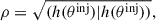
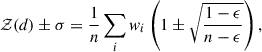
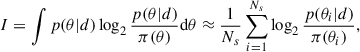
We defined the metrics to evaluate the performance in estimating parameters of the various configurations of XG detectors. The information gain (I) is defined as the Kullback–Leibler (KL) divergence (Kullback & Leibler 1951) between the prior and the posterior (Buchner 2022). In particular, we computed the KL divergence of the posterior from the prior:
 (3)
(3)
which quantifies the extent to which the prior volume has been constrained by the data, i.e., by a factor of 2I (Skilling 2004). As opposed to single- or few-parameter metrics, the information gain fully characterizes the size of the 11-dimensional posterior distribution, accounting for correlations across any parameters. Equation (3) was evaluated using a Monte Carlo integral. Additional details on this are provided in Appendix E.
Because DINGO-IS provides full parameter estimates for each source, we can define precise metrics to assess how different detector networks perform in source localization. For each event, we computed the area (in deg2) enclosed by the smallest 90% confidence region. The sky maps were sampled using equal-area HEALPix (Hierarchical Equal Area isoLatitude Pixelization) pixels (Gorski et al. 1999; Górski et al. 2005), where each of the N pixels carries a posterior probability (pi) that the source lies within that pixel.
We employed the ligo-skymap library (Singer & Price 2016; Singer et al. 2016a,b), which also identifies the number of disconnected sky modes (or probability islands) within a given area using a flood-fill algorithm (Foley et al. 1996), which finds all pixels connected to a starting one. Additionally, by including the posterior on luminosity distance, we computed the 90% highest probability density comoving volume ( ; see Sect. 3 of Singer et al. 2016a).
The other reported interval widths, for example Δx/xinj, indicate the relative variation of a parameter from its injected value. Here, Δx corresponds to the square root of the associated covariance matrix element and represents the 1σ uncertainty of the parameter estimate.
3. Results
3.1. High signal-to-noise ratio versus high sample efficiency
We generated 1000 sets of BBH merger parameters sampled from the prior and used the same samples for all configurations. From the DINGO proposal distribution qϕ(θ|d), we drew 105 posterior samples and computed the corresponding importance weights (see Sect. 2.2). For each injected signal, we then evaluated the sample efficiency. To ensure unbiased estimates of the inferred parameters, we required at least 103 effective samples per source, corresponding to a sample efficiency > 1%.
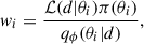
The top panel of Fig. 1 shows that a large fraction of injected signals achieves a sample efficiency greater than 1%, ranging from 96% for Δ and 2L A configurations to a minimum of 85% for 2L MisA + CE. These values remain consistently high, with even better performance for the Δ configuration than previously reported in Santoliquido et al. (2025). This improvement arises from the increased dimensionality of the embedding network (see Sect. 2.2), emphasizing the crucial role of this component within the NPE framework.
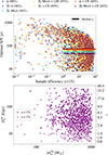 |
Fig. 1. Top panel: Injections as a function of sample efficiency (ϵ, x-axis) and optimal S/N (ρ, y-axis) for each detector configuration (color-coded). Filled markers indicate injections with sample efficiencies > 1%. Percentages in parentheses denote the fraction of sources with a sample efficiency above 1%, while the horizontal colored lines indicate the median ρ for sources exceeding this threshold. Bottom panel: Injections as a function of detector-frame chirp mass (x-axis) and luminosity distance (left y-axis), with corresponding redshifts (right y-axis). Colored markers indicate events with a sample efficiency greater than 1% in all considered detector configurations. See Sect. 3.1 for details. |
The top panel of Fig. 1 also shows that 50% of the events have an optimal signal-to-noise ratio (S/N; see Appendix D) exceeding 40 for the Δ configuration and up to 70 for 2L MisA + CE, while still achieving sample efficiencies above 1%. This demonstrates that the sample efficiency remains high even for high-S/N events, indicating that NPE may represent a promising approach to addressing the parameter estimation challenges posed by XG detectors.
To ensure an unbiased evaluation of parameter estimation performance, we included only injections with sample efficiencies exceeding 1% across all seven detector configurations. We further restricted the dataset to sources with optimal S/N ρ > 8. The bottom panel of Fig. 1 illustrates the parameter space of the retained sources, which account for 78% of the total, showing that events with ℳd ≲ 150 M⊙ and DL ≲ 6 Gpc are almost entirely excluded. These sources have low sample efficiencies because their high S/N makes them more challenging for NPE to model, as their posteriors are much narrower than the prior. This behavior is further evident in the top panel of Fig. 1, where sample efficiency drops sharply for sources with optimal S/Ns of around ∼1000.
We are currently exploring several strategies to improve sample efficiency in regions of parameter space where performance remains below the threshold, including training DINGO-IS with neural population priors (e.g., Wouters et al. 2025). The results of these efforts will be presented in future work.
3.2. Multimodal posterior of a single event
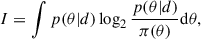
The top panel of Fig. 2 shows that DINGO-IS yields posterior distributions that are statistically indistinguishable from those obtained using BILBY (see Appendix D for a formal validation). Crucially, this accuracy is achieved at a dramatically lower computational cost: DINGO-IS requires only a few minutes per source, whereas BILBY needs more than 22 hours (50 hours) to converge for this event with the Δ (2L MisA) configuration.
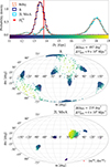 |
Fig. 2. Top panel: Marginalized one-dimensional posterior distributions for the luminosity distance, recovered with DINGO-IS, for an event observed with the Δ (dark blue) and 2L MisA (light blue) configurations. The results are compared with BILBY (orange). The vertical line marks the injected luminosity distance. The remaining parameters are shown in Appendix D. Middle panel: Posterior samples obtained with DINGO-IS in the Δ configuration for right ascension (ra) and declination (dec), color-coded by luminosity distance. The red cross marks the injected sky position. We also report the sky-localization area (ΔΩ90%) and comoving-volume localization (ΔV90%c) errors. Bottom panel: Same as the middle panel but for the 2L MisA configuration. See Sect. 3.2 for details. |
Figure 2 also shows that DINGO-IS accurately captures the complex structure of multimodal posteriors. These multimodalities include both the eight-fold sky degeneracy arising from the triangular geometry of ET, extensively discussed in Santoliquido et al. (2025), and modes introduced by the 2L MisA configuration, which affect both sky localization and luminosity distance.
The bottom panel of Fig. 2 shows that for the 2L MisA configuration, the sky location is correlated with luminosity distance: distinct islands of probability on the sky correspond to different modes in DL. For this source, we identify three such modes. The occurrence rate of multimodal posteriors in luminosity distance is discussed in Appendix F and shown in Fig. F.1. The 2L MisA (2L A) configurations produce a multimodal DL posterior more frequently than the Δ configuration, with rates of about 20% compared to ∼2%. In Appendix G we show that the multimodalities in luminosity distance and sky localization observed for the 2L configurations are robust features, persisting across different waveform approximants.
These multimodalities are expected when observing short-duration, high-mass BBHs with both the 2L A and 2L MisA configurations of ET. They arise from the combined effect of the short baseline between the two interferometers (∼1000 km) and the low merger frequencies of massive BBHs (typically ≲50 Hz). We provide an illustrative example in Appendix H, showing that for a signal with higher merger frequencies, the multimodalities in both sky position and distance disappear.
Despite the multimodality in DL, the number of sky-position modes is significantly reduced compared to the triangular configuration, resulting in improved sky-area and comoving-volume localization for the 2L MisA configuration. Additional details, including the same source as observed with the 2L MisA + CE configuration, are provided in Appendix D.
3.3. Parameter estimation performance
The top-left panel of Fig. 3 shows the parameter estimation performance of the considered detector configurations, measured by the information gain, revealing a clear ranking. Among the ET configurations (Δ, 2L A, and 2L MisA), when no other XG detectors are observing simultaneously, the 2L MisA setup performs best. Moreover, adding three LIGO observatories operating at A# sensitivity to the 2L MisA configuration further increases the information gain, underscoring the capability of this global network to estimate the parameters of the specific sources examined in this study – namely, both massive and high-redshift BBHs. The information gain further increases when 1L ET observes jointly with CE, as the longer baseline enhances both sky and volume localization. However, the separation between the 2L MisA detectors also plays a role: when observing together with CE, the 2L MisA + CE configuration outperforms Δ + CE.
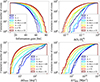 |
Fig. 3. Cumulative distributions of events as a function of the information gain (top-left panel; see also Sect. 2.3), the relative variation in luminosity distance (top-right panel; |


The top-right panel of Fig. 3 shows that the luminosity distance is best measured with the Δ configuration, outperforming both the 2L A and 2L MisA configurations. Compared to Branchesi et al. (2023, see their Fig. 5), we find a reversed hierarchy in detector performance. We stress that our analysis is restricted to both massive and high-redshift BBH mergers. For this class of source, the 2L configurations give rise to multimodal posteriors in DL (see Fig. 2 and Appendix F), an effect that is not captured with Fisher-matrix-based analyses.
Nevertheless, the 2L MisA configuration leads to better sky and volume localization, allowing it to outperform the Δ and 2L A setup in these metrics (bottom panels of Fig. 3). Improving the accuracy of the localization volume critically enhances the prospects for dark siren cosmology, which relies on the statistical association between the GW source and galaxies contained within the reconstructed localization volume (Schutz 1986; Del Pozzo 2012; Chen et al. 2018; Libanore et al. 2021; Gair et al. 2023; Bosi et al. 2023; Borghi et al. 2024).
Table 1 summarizes the sky localization performance for all detector configurations, showing a clear improvement from the 2L A configuration, which performs worst, to 2L MisA + CE, which achieves the best results. In the latter case, more than 70% of sources are localized within 100 deg2.
Percentage of injections (color-coded) with estimated sky localization errors within the specified areas (columns) for different detector configurations (rows).
Figure 4 shows that more than 80% of events exhibit eight sky modes in the Δ configuration. This fraction is substantially reduced for the two L-shaped detector configurations: in the 2L MisA setup, the occurrence of eight sky modes drops to about 20% of the events. The 2L MisA configuration exhibits an eight-sky-mode pattern for events located close to the local horizon defined at the midpoint between the two L-shaped interferometers. For such events, the time-of-arrival difference is negligible, effectively making the two interferometers colocated (Marsat et al. 2021).
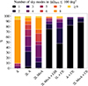 |
Fig. 4. Percentage of sky maps (y-axis) with ΔΩ90% ≤ 100 deg2 exhibiting one to eight or more disconnected modes (color-coded), for all detector configurations (x-axis). See Sect. 3.3 for details. |
The 2L A setup localizes nearly 30% of the sources in two distinct sky modes, outperforming the 2L MisA configuration, for which this fraction remains below 10%. However, the average sky-localization area per mode is significantly larger in 2L A compared to 2L MisA. None of the ET configurations are able to localize events in a single sky mode unless ET operates as part of a global network that includes either the three LIGO interferometers at A# sensitivity (including LIGO–India) or CE.
For completeness, Fig. 5 presents the performance of the considered detector configurations in estimating the remaining parameters, such as optimal S/N, detector-frame chirp mass, mass ratio, the aligned spin components, and inclination angle. The overall trend is confirmed, as the Δ and 2L A configurations provide the poorest performance, while the 2L MisA + CE setup delivers the most accurate estimates.
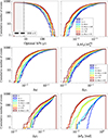 |
Fig. 5. Cumulative distributions of events as a function of the optimal S/N (ρ; Eq. (D.4)), the relative variations in detector-frame chirp mass ( |

The performance of ET configurations in estimating parameters of compact binary coalescences arises from the interplay between polarization measurements and a baseline that enables triangulation (Fairhurst 2009). Breaking the degeneracy between DL and θjn requires measuring both polarizations (Usman et al. 2019), and the ability to do so is quantified by the alignment factor (Klimenko et al. 2006; de Souza & Sturani 2023; Mascioli et al. 2025). A network composed of two L-shaped interferometers that are perfectly aligned provides no information on the cross-polarization. In contrast, the Δ configuration exhibits the highest alignment factor, yielding the most accurate polarization measurements. However, the sky maps produced by this configuration feature eight distinct sky modes owing to the colocated nature of the detectors (Singh & Bulik 2021, 2022; Santoliquido et al. 2025). As a result, the 2L MisA configuration offers a tradeoff, enabling polarization measurements while reducing the number of sky modes (see Fig. 4).
4. Conclusions
Given the unique sensitivity that ET and other XG GW detectors will provide for early-Universe stellar and PBHs, as well as IMBH binaries, we focused our analysis on BBH mergers with detector-frame chirp masses (ℳd) > 100 M⊙. Although this study addresses a more restricted science case than the full range of sources observable with XG detectors (Branchesi et al. 2023; Abac et al. 2025a), it targets a regime with strong potential for breakthrough discoveries.
We assessed the performance of seven configurations of XG detectors using NPE enhanced with importance sampling, as implemented in DINGO-IS (Dax et al. 2023). We conduced a large injection campaign by sampling 1000 BBH merger parameters from the prior. As shown in Fig. 1, DINGO-IS achieves excellent performance, recovering 85–96% of signals with a sample efficiency above 1%, depending on the detector configuration, for median S/Ns between 40 and 70. This demonstrates that its efficiency remains high even for high-S/N events.
In Sect. 3.2 we present a single-injection study showing that DINGO-IS accurately reproduces complex, disconnected posteriors consistent with standard stochastic-sampling methods but at a fraction of the computational cost – a few minutes instead of several hours. Our analysis shows that a network of two misaligned L-shaped ET detectors (2L MisA) can produce multimodal luminosity–distance posteriors (see the top panel of Fig. 2), and its distance estimates are generally less precise than those obtained with the triangular ET design (Δ). However, Fig. 3 demonstrates that the 2L MisA outperforms the Δ configuration in terms of information gain, sky localization, and volume reconstruction. The Δ configuration’s larger number of sky modes leads to poorer sky-localization performance, which in turn dominates its volume uncertainty.
For both high-mass and high-redshift BBH events, the fraction of sources recovered within a single sky mode remains low for all ET configurations (Δ, 2L A, and 2L MisA). It surpasses 50% when CE is added to the global XG network and exceeds 70% when, instead, three LIGO detectors operate at A# sensitivity, as shown in Fig. 4.
Data availability
The data used in this study are publicly available on Zenodo. The dataset corresponding to the Δ configuration can be found at https://zenodo.org/records/18911700; the datasets for the 2L A, 2L MisA, and Δ + CE configurations are available at https://zenodo.org/records/18911495; and the datasets for 2L MisA + LHI, 1L + CE, and 2L MisA + CE are available at https://zenodo.org/records/18911380. The latest public release of DINGO is available at https://github.com/dingo-gw/dingo; this work is based on commit DF6E586 in the fork DINGO-ET (https://github.com/filippo-santoliquido/dingo-ET). Additional data and code are available from the corresponding authors upon reasonable request.
Acknowledgments
We thank the anonymous referee for their thorough and careful review of our manuscript. We thank Stephen R. Green, Francesco Iacovelli, Luca Reali, Alexandre Toubiana, Manuel Arca Sedda, Michele Maggiore, Archisman Gosh, Elisa Maggio and Emanuele Berti for useful discussions. F.S. has been funded by the European Union – NextGenerationEU under the Italian Ministry of University and Research (MUR) “Decreto per l’assunzione di ricercatori internazionali post-dottorato PNRR” – Missione 4 “Istruzione e Ricerca” Componente 2 “Dalla Ricerca all’Impresa” del PNRR – Investimento 1.2 “Finanziamento di progetti presentati da giovani ricercatori” – CUP D13C25000700001. M.B. and J.H. acknowledge support from the Astrophysics Center for Multi-messenger Studies in Europe (ACME), funded under the European Union’s Horizon Europe Research and Innovation Program, Grant Agreement No. 101131928. The data analysis has been performed on the HPC workstations “Merac2A” financially supported by the MERAC Foundation and the European Astronomical Society through the 2023 MERAC Prize and the MERAC Support to research (PI Manuel Arca Sedda). The research leading to these results has been conceived and developed within the Einstein Telescope Observational Science Board ET-0611A-25.
References
- Abac, A., Abramo, R., Albanesi, S., et al. 2025a, arXiv e-prints [arXiv:2503.12263] [Google Scholar]
- Abac, A. G., Abouelfettouh, I., Acernese, F., et al. 2025b, ApJ, 993, L25 [Google Scholar]
- Abac, A. G., Abouelfettouh, I., Acernese, F., et al. 2025c, Phys. Rev. Lett., 135, 111403 [Google Scholar]
- Ajith, P., Hannam, M., Husa, S., et al. 2011, Phys. Rev. Lett., 106, 241101 [NASA ADS] [CrossRef] [Google Scholar]
- Alléné, C., Aubin, F., Bentara, I., et al. 2025, Class. Quant. Grav., 42, 105009 [Google Scholar]
- Antonini, F., Gieles, M., & Gualandris, A. 2019, MNRAS, 486, 5008 [NASA ADS] [CrossRef] [Google Scholar]
- Arca Sedda, M., Amaro Seoane, P., & Chen, X. 2021, A&A, 652, A54 [NASA ADS] [CrossRef] [EDP Sciences] [Google Scholar]
- Arca Sedda, M., Kamlah, A. W. H., Spurzem, R., et al. 2023, MNRAS, 526, 429 [NASA ADS] [CrossRef] [Google Scholar]
- Ashton, G. 2025, arXiv e-prints [arXiv:2510.11197] [Google Scholar]
- Ashton, G., Huebner, M., Lasky, P. D., et al. 2019, ApJS, 241, 27 [NASA ADS] [CrossRef] [Google Scholar]
- Aubin, F., Brighenti, F., Chierici, R., et al. 2021, Class. Quant. Grav., 38, 095004 [Google Scholar]
- Baibhav, V., Berti, E., Gerosa, D., et al. 2019, Phys. Rev. D, 100, 064060 [NASA ADS] [CrossRef] [Google Scholar]
- Belczynski, K., Ryu, T., Perna, R., et al. 2017, MNRAS, 471, 4702 [Google Scholar]
- Bini, S., Król, K., Chatziioannou, K., & Isi, M. 2026, arXiv e-prints [arXiv:2601.09678] [Google Scholar]
- Blackman, J., Field, S. E., Galley, C. R., et al. 2015, Phys. Rev. Lett., 115, 121102 [Google Scholar]
- Blinnikov, S., Dolgov, A., Porayko, N. K., & Postnov, K. 2016, JCAP, 11, 036 [Google Scholar]
- Borghi, N., Mancarella, M., Moresco, M., et al. 2024, ApJ, 964, 191 [Google Scholar]
- Bosi, M., Bellomo, N., & Raccanelli, A. 2023, JCAP, 11, 086 [Google Scholar]
- Branchesi, M., Maggiore, M., Alonso, D., et al. 2023, JCAP, 07, 068 [CrossRef] [Google Scholar]
- Buchner, J. 2022, Res. Notes AAS, 6, 89 [Google Scholar]
- Buonanno, A., & Damour, T. 1999, Phys. Rev. D, 59, 084006 [Google Scholar]
- Buonanno, A., & Damour, T. 2000, Phys. Rev. D, 62, 064015 [Google Scholar]
- Buonanno, A., Pan, Y., Baker, J. G., et al. 2007, Phys. Rev. D, 76, 104049 [Google Scholar]
- Canizares, P., Field, S. E., Gair, J., et al. 2015, Phys. Rev. Lett., 114, 071104 [Google Scholar]
- Carr, B. J. 1975, ApJ, 201, 1 [NASA ADS] [CrossRef] [Google Scholar]
- Carr, B., Kohri, K., Sendouda, Y., & Yokoyama, J. 2021, Rept. Prog. Phys., 84, 116902 [Google Scholar]
- CE Collaboration. 2022, CE 40-km baseline noise curve, https://dcc.cosmicexplorer.org/CE-T2000017/public [Google Scholar]
- Chan, J. C. L., Magaña Zertuche, L., Ezquiaga, J. M., et al. 2026, Phys. Rev. D, 113, 024041 [Google Scholar]
- Chapline, G. F. 1975, Nature, 253, 251 [NASA ADS] [CrossRef] [Google Scholar]
- Chatterjee, C., Kovalam, M., Wen, L., et al. 2023, ApJ, 959, 42 [Google Scholar]
- Chatziioannou, K., Dent, T., Fishbach, M., et al. 2024, arXiv e-prints [arXiv:2409.02037] [Google Scholar]
- Chen, H.-Y., Fishbach, M., & Holz, D. E. 2018, Nature, 562, 545 [Google Scholar]
- Christensen, N., & Meyer, R. 2022, Rev. Mod. Phys., 94, 025001 [NASA ADS] [CrossRef] [Google Scholar]
- Colleoni, M., Vidal, F. A. R., García-Quirós, C., Akçay, S., & Bera, S. 2025, Phys. Rev. D, 111, 104019 [Google Scholar]
- Cook, Samantha R. A. G. & Rubin, D. B. J. Comput. Graphical, 2006, Stat., 15, 675 [Google Scholar]
- Cornish, N. J. 2010, arXiv e-prints [arXiv:1007.4820] [Google Scholar]
- Cuoco, E., Powell, J., Cavaglià, M., et al. 2021, Mach. Learn.: Sci. Technol., 2, 011002 [Google Scholar]
- Dax, M., Green, S. R., Gair, J., et al. 2021a, arXiv e-prints [arXiv:2111.13139] [Google Scholar]
- Dax, M., Green, S. R., Gair, J., et al. 2021b, Phys. Rev. Lett., 127, 241103 [NASA ADS] [CrossRef] [Google Scholar]
- Dax, M., Green, S. R., Gair, J., et al. 2023, Phys. Rev. Lett., 130, 171403 [NASA ADS] [CrossRef] [Google Scholar]
- De Luca, V., Franciolini, G., Pani, P., & Riotto, A. 2020, JCAP, 06, 044 [CrossRef] [Google Scholar]
- De Santi, F., Razzano, M., Fidecaro, F., et al. 2024, Phys. Rev. D, 109, 102004 [Google Scholar]
- de Souza, J. M. S., & Sturani, R. 2023, Phys. Rev. D, 108, 043027 [Google Scholar]
- Del Pozzo, W. 2012, Phys. Rev. D, 86, 043011 [NASA ADS] [CrossRef] [Google Scholar]
- Dupletsa, U. 2025, Tutorial on GWFish+Priors, https://github.com/janosch314/GWFish/blob/main/priors_tutorial.ipynb, accessed: March 11, 2025 [Google Scholar]
- Elvira, V., & Martino, L. 2021, Advances in Importance Sampling (Wiley) [Google Scholar]
- ET Collaboration. 2023, ET 10-km and 15-km noise curve, https://apps.et-gw.eu/tds/?r=18213 [Google Scholar]
- Evans, M., Corsi, A., Afle, C., et al. 2023, arXiv e-prints [arXiv:2306.13745] [Google Scholar]
- Fairhurst, S. 2009, New J. Phys., 11, 123006 [Erratum: New J. Phys., 13, 069602 (2011)] [Google Scholar]
- Field, S. E., Galley, C. R., Hesthaven, J. S., Kaye, J., & Tiglio, M. 2014, Phys. Rev. X, 4, 031006 [Google Scholar]
- Finn, L. S. 1992, Phys. Rev. D, 46, 5236 [NASA ADS] [CrossRef] [Google Scholar]
- Fishbach, M., Holz, D. E., & Farr, B. 2017, ApJ, 840, L24 [NASA ADS] [CrossRef] [Google Scholar]
- Foley, J. D., van Dam, A., Feiner, S. K., & Hughes, J. F. 1996, Computer Graphics: Principles and Practice, 2nd edn. (Addison-Wesley) [Google Scholar]
- Franciolini, G., Musco, I., Pani, P., & Urbano, A. 2022, Phys. Rev. D, 106, 123526 [NASA ADS] [CrossRef] [Google Scholar]
- Franciolini, G., Iacovelli, F., Mancarella, M., et al. 2023, Phys. Rev. D, 108, 043506 [NASA ADS] [CrossRef] [Google Scholar]
- Gair, J. R., Ghosh, A., Gray, R., et al. 2023, AJ, 166, 22 [NASA ADS] [CrossRef] [Google Scholar]
- Gerosa, D., & Berti, E. 2017, Phys. Rev. D, 95, 124046 [NASA ADS] [CrossRef] [Google Scholar]
- Gerosa, D., & Fishbach, M. 2021, Nat. Astron., 5, 749 [NASA ADS] [CrossRef] [Google Scholar]
- Giersz, M., Leigh, N., Hypki, A., et al. 2015, MNRAS, 454, 3150 [Google Scholar]
- Gorski, K. M., Wandelt, B. D., Hansen, F. K., Hivon, E., & Banday, A. J. 1999, arXiv e-prints [arXiv:astro-ph/9905275] [Google Scholar]
- Górski, K. M., Hivon, E., Banday, A. J., et al. 2005, ApJ, 622, 759 [Google Scholar]
- Green, S. R., & Gair, J. 2021, Mach. Learn. Sci. Technol., 2, 03LT01 [Google Scholar]
- Green, S. R., Simpson, C., & Gair, J. 2020, Phys. Rev. D, 102, 104057 [NASA ADS] [CrossRef] [Google Scholar]
- Gültekin, K., Miller, M. C., & Hamilton, D. P. 2004, ApJ, 616, 221 [Google Scholar]
- Gupta, I., Afle, C., Arun, K., et al. 2024, Class. Quant. Grav., 41, 245001 [Google Scholar]
- Guth, A. H., & Sfakianakis, E. I. 2012, arXiv e-prints [arXiv:1210.8128] [Google Scholar]
- Hall, E. D., & Evans, M. 2019, Class. Quant. Grav., 36, 225002 [NASA ADS] [CrossRef] [Google Scholar]
- Hartigan, P. M. 1985, J. R. Stat. Soc. Ser. C (Appl. Stat.), 34, 320 [Google Scholar]
- Hartigan, J. A., & Hartigan, P. M. 1985, Ann. Stat., 13, 70 [Google Scholar]
- Hartwig, T., Volonteri, M., Bromm, V., et al. 2016, MNRAS, 460, L74 [NASA ADS] [CrossRef] [Google Scholar]
- Hawking, S. W. 1974, Nature, 248, 30 [CrossRef] [Google Scholar]
- Heinzel, J., & Vitale, S. 2025, arXiv e-prints [arXiv:2509.07221] [Google Scholar]
- Hu, Q., & Veitch, J. 2025, Phys. Rev. D, 112, 084039 [Google Scholar]
- Ivanov, P. 1998, Phys. Rev. D, 57, 7145 [NASA ADS] [CrossRef] [Google Scholar]
- Ivanov, P., Naselsky, P., & Novikov, I. 1994, Phys. Rev. D, 50, 7173 [CrossRef] [Google Scholar]
- Kandhasamy, S., & Bose, S. 2020, LIGO India Observatory (LIO) coordinate system for GW analyses, https://dcc.ligo.org/public/0167/T2000158/001/LIO_coordinateSystem.pdf [Google Scholar]
- Kinugawa, T., Nakamura, T., & Nakano, H. 2020, MNRAS, 498, 3946 [NASA ADS] [CrossRef] [Google Scholar]
- Klimenko, S., Mohanty, S., Rakhmanov, M., & Mitselmakher, G. 2006, J. Phys. Conf. Ser., 32, 12 [CrossRef] [Google Scholar]
- Kobyzev, I., Prince, S. J., & Brubaker, M. A. 2021, IEEE Trans. Pattern Anal. Mach. Intell., 43, 3964 [NASA ADS] [CrossRef] [Google Scholar]
- Kofler, A., Dax, M., Green, S. R., et al. 2025, arXiv e-prints [arXiv:2512.02968] [Google Scholar]
- Kong, A. 1992, A Note on Importance Sampling using Standardized Weights (University of Chicago, Dept. of Statistics), Tech. Rep 384 [Google Scholar]
- Kritos, K., Strokov, V., Baibhav, V., & Berti, E. 2024, Phys. Rev. D, 110, 043023 [Google Scholar]
- Kullback, S., & Leibler, R. A. 1951, Ann. Math. Stat., 22, 79 [CrossRef] [Google Scholar]
- Lanchares, D., Freitas, O. G., González-Nuevo, J., & Font, J. A. 2025, arXiv e-prints [arXiv:2505.08089] [Google Scholar]
- Lange, J., O’Shaughnessy, R., & Rizzo, M. 2018, arXiv e-prints [arXiv:1805.10457] [Google Scholar]
- Langendorff, J., Kolmus, A., Janquart, J., & Van Den Broeck, C. 2023, Phys. Rev. Lett., 130, 171402 [Google Scholar]
- Leslie, N., Dai, L., & Pratten, G. 2021, Phys. Rev. D, 104, 123030 [Google Scholar]
- Libanore, S., Artale, M. C., Karagiannis, D., et al. 2021, JCAP, 02, 035 [Google Scholar]
- LIGO Collaboration. 2020, A# sensitivity curve, https://dcc.ligo.org/LIGO-T2300041/public [Google Scholar]
- Lin, J. 1991, IEEE Trans. Inf. Theory, 37, 145 [Google Scholar]
- Liu, B., & Bromm, V. 2020, MNRAS, 495, 2475 [NASA ADS] [CrossRef] [Google Scholar]
- Mackay, D. J. C. 2003, Information Theory, Inference and Learning Algorithms (Cambridge University Press) [Google Scholar]
- Maggiore, M., Broeck, C. V. D., Bartolo, N., et al. 2020, J. Cosmol. Astropart. Phys., 2020, 050 [CrossRef] [Google Scholar]
- Maggiore, M., Iacovelli, F., Belgacem, E., Mancarella, M., & Muttoni, N. 2025, Class. Quant. Grav., 42, 215004 [Google Scholar]
- Mapelli, M. 2016, MNRAS, 459, 3432 [NASA ADS] [CrossRef] [Google Scholar]
- Marsat, S., Baker, J. G., & Dal Canton, T. 2021, Phys. Rev. D, 103, 083011 [NASA ADS] [CrossRef] [Google Scholar]
- Marx, E., Chatterjee, D., Desai, M., et al. 2025, arXiv e-prints [arXiv:2509.22561] [Google Scholar]
- Mascioli, A. F., Crescimbeni, F., Pacilio, C., Pani, P., & Pannarale, F. 2025, Phys. Rev. D, 112, 062003 [Google Scholar]
- Mestichelli, B., Mapelli, M., Torniamenti, S., et al. 2024, A&A, 690, A106 [NASA ADS] [CrossRef] [EDP Sciences] [Google Scholar]
- Miller, M. C., & Hamilton, D. P. 2002, MNRAS, 330, 232 [Google Scholar]
- Morisaki, S. 2021, Phys. Rev. D, 104, 044062 [Google Scholar]
- Morras, G., Siles, J. F. N., & Garcia-Bellido, J. 2023, Phys. Rev. D, 108, 123025 [CrossRef] [Google Scholar]
- Narola, H., Janquart, J., Meijer, Q., Haris, K., & Van Den Broeck, C. 2024, Phys. Rev. D, 110, 084085 [Google Scholar]
- Narola, H., Wouters, T., Negri, L., et al. 2025, Phys. Rev. D, 112, 024079 [Google Scholar]
- Negri, L., & Samajdar, A. 2025, arXiv e-prints [arXiv:2509.17606] [Google Scholar]
- Ng, K. K. Y., Franciolini, G., Berti, E., et al. 2022, ApJ, 933, L41 [NASA ADS] [CrossRef] [Google Scholar]
- Owen, A. B. 2013, Monte Carlo theory, methods and examples, https://artowen.su.domains/mc/ [Google Scholar]
- Papamakarios, G., Nalisnick, E., Rezende, D. J., Mohamed, S., & Lakshminarayanan, B. 2021, J. Mach. Learn. Res., 22, 2617 [Google Scholar]
- Payne, E., Talbot, C., & Thrane, E. 2019, Phys. Rev. D, 100, 123017 [NASA ADS] [CrossRef] [Google Scholar]
- Perret, J., Aréne, M., & Porter, E. K. 2025, arXiv e-prints [arXiv:2505.02589] [Google Scholar]
- Planck Collaboration VI. 2020, A&A, 641, A6, [Erratum: A&A 652, C4 (2021)] [NASA ADS] [CrossRef] [EDP Sciences] [Google Scholar]
- Portegies Zwart, S. F., & McMillan, S. L. W. 2002, ApJ, 576, 899 [Google Scholar]
- Prathaban, M., Bevins, H., & Handley, W. 2025a, MNRAS, 541, 200 [Google Scholar]
- Prathaban, M., Yallup, D., Alvey, J., et al. 2025b, arXiv e-prints [arXiv:2509.04336] [Google Scholar]
- Pratten, G., García-Quirós, C., Colleoni, M., et al. 2021, Phys. Rev. D, 103, 104056 [NASA ADS] [CrossRef] [Google Scholar]
- Punturo, M., Abernathy, M., Acernese, F., et al. 2010, Class. Quant. Grav., 27, 194002 [Google Scholar]
- Ramos-Buades, A., Buonanno, A., & Gair, J. 2023, Phys. Rev. D, 108, 124063 [Google Scholar]
- Reitze, D., Adhikari, R. X., Ballmer, S., et al. 2019, Bull. Am. Astron. Soc., 51, 035 [Google Scholar]
- Rizzuto, F. P., Naab, T., Rantala, A., et al. 2023, MNRAS, 521, 2930 [NASA ADS] [CrossRef] [Google Scholar]
- Romano, J. D., & Cornish, N. J. 2017, Liv. Rev. Relat., 20, 2 [CrossRef] [Google Scholar]
- Romero-Shaw, I. M., Talbot, C., Biscoveanu, S., et al. 2020, MNRAS, 499, 3295 [NASA ADS] [CrossRef] [Google Scholar]
- Rubin, D. B. 1988, in Bayesian Statistics 3, eds. J. M. Bernardo, M. H. de Groot, D. V. Lindley, & A. F. M. Smith (Oxford, UK: Oxford University Press), 395 [Google Scholar]
- Santoliquido, F., Mapelli, M., Iorio, G., et al. 2023, MNRAS, 524, 307 [NASA ADS] [CrossRef] [Google Scholar]
- Santoliquido, F., Dupletsa, U., Tissino, J., et al. 2024, A&A, 690, A362 [NASA ADS] [CrossRef] [EDP Sciences] [Google Scholar]
- Santoliquido, F., Tissino, J., Dupletsa, U., et al. 2025, Phys. Rev. D, 112, 103015 [Google Scholar]
- Schutz, B. F. 1986, Nature, 323, 310 [Google Scholar]
- Singer, L. P., & Price, L. R. 2016, Phys. Rev. D, 93, 024013 [CrossRef] [Google Scholar]
- Singer, L. P., Chen, H.-Y., Holz, D. E., et al. 2016a, ApJ, 829, L15 [NASA ADS] [CrossRef] [Google Scholar]
- Singer, L. P., Chen, H.-Y., Holz, D. E., et al. 2016b, ApJS, 226, 10 [NASA ADS] [CrossRef] [Google Scholar]
- Singh, N., & Bulik, T. 2021, Phys. Rev. D, 104, 043014 [NASA ADS] [CrossRef] [Google Scholar]
- Singh, N., & Bulik, T. 2022, Phys. Rev. D, 106, 123014 [NASA ADS] [CrossRef] [Google Scholar]
- Skilling, J. 2004, AIP Conf. Proc., 735, 395 [Google Scholar]
- Smith, R. J. E., Ashton, G., Vajpeyi, A., & Talbot, C. 2020, MNRAS, 498, 4492 [Google Scholar]
- Smith, R., Borhanian, S., Sathyaprakash, B., et al. 2021, Phys. Rev. Lett., 127, 081102 [Google Scholar]
- Srinivasan, R., Barausse, E., Korsakova, N., & Trotta, R. 2025, Phys. Rev. D, 112, 103043 [Google Scholar]
- Stone, N. C., Küpper, A. H. W., & Ostriker, J. P. 2017, MNRAS, 467, 4180 [NASA ADS] [Google Scholar]
- Talbot, C., & Golomb, J. 2023, MNRAS, 526, 3495 [NASA ADS] [CrossRef] [Google Scholar]
- Talts, S., Betancourt, M., Simpson, D., Vehtari, A., & Gelman, A. 2020, Validating Bayesian Inference Algorithms with Simulation-Based Calibration, https://arxiv.org/abs/1804.06788 [Google Scholar]
- Tanikawa, A., Chiaki, G., Kinugawa, T., Suwa, Y., & Tominaga, N. 2022, PASJ, 74, 521 [NASA ADS] [CrossRef] [Google Scholar]
- Thompson, J. E., Hamilton, E., London, L., et al. 2024, Phys. Rev. D, 109, 063012 [Google Scholar]
- Thrane, E., & Talbot, C. 2019, PASA, 36, e010 [Erratum: PASA, 37, e036 (2020)] [NASA ADS] [CrossRef] [Google Scholar]
- Tissino, J., Carullo, G., Breschi, M., et al. 2023, Phys. Rev. D, 107, 084037 [CrossRef] [Google Scholar]
- Tokdar, S. T., & Kass, R. E. 2010, WIREs Comp. Stats., 2, 54 [Google Scholar]
- Unnikrishnan, C. S. 2013, Int. J. Mod. Phys. D, 22, 1341010 [Google Scholar]
- Usman, S. A., Mills, J. C., & Fairhurst, S. 2019, ApJ, 877, 82 [NASA ADS] [CrossRef] [Google Scholar]
- van der Sluys, M. V., Röver, C., Stroeer, A., et al. 2008, ApJ, 688, L61 [Google Scholar]
- van der Sluys, M., Mandel, I., Raymond, V., et al. 2009, Class. Quant. Grav., 26, 204010 [Google Scholar]
- Varma, V., Field, S. E., Scheel, M. A., et al. 2019, Phys. Rev. Res., 1, 033015 [NASA ADS] [CrossRef] [Google Scholar]
- Varma, V., Isi, M., Biscoveanu, S., Farr, W. M., & Vitale, S. 2022, Phys. Rev. D, 105, 024045 [Google Scholar]
- Veitch, J., Raymond, V., Farr, B., et al. 2015, Phys. Rev. D, 91, 042003 [NASA ADS] [CrossRef] [Google Scholar]
- Vinciguerra, S., Veitch, J., & Mandel, I. 2017, Class. Quant. Grav., 34, 115006 [Google Scholar]
- Wang, L., Tanikawa, A., & Fujii, M. 2022, MNRAS, 515, 5106 [NASA ADS] [CrossRef] [Google Scholar]
- Wildberger, J. B., Dax, M., Buchholz, S., et al. 2023, in Machine Learning for Astrophysics, 34 [Google Scholar]
- Williams, M. J. 2021, https://doi.org/10.5281/zenodo.4550693 [Google Scholar]
- Williams, M. J., Veitch, J., & Messenger, C. 2021, Phys. Rev. D, 103, 103006 [NASA ADS] [CrossRef] [Google Scholar]
- Williams, M. J., Veitch, J., & Messenger, C. 2023, Mach. Learn.: Sci. Technol., 4, 035011 [NASA ADS] [CrossRef] [Google Scholar]
- Wong, K. W. K., Gabrié, M., & Foreman-Mackey, D. 2023a, J. Open Source Softw., 8, 5021 [Google Scholar]
- Wong, K. W. K., Isi, M., & Edwards, T. D. P. 2023b, ApJ, 958, 129 [NASA ADS] [CrossRef] [Google Scholar]
- Wouters, T., Pang, P. T. H., Dietrich, T., & Van Den Broeck, C. 2024, Phys. Rev. D, 110, 083033 [NASA ADS] [CrossRef] [Google Scholar]
- Wouters, T., Pang, P. T. H., Dietrich, T., & Van Den Broeck, C. 2025, arXiv e-prints [arXiv:2511.22987] [Google Scholar]
- Zackay, B., Dai, L., & Venumadhav, T. 2018, arXiv e-prints [arXiv:1806.08792] [Google Scholar]
- Zel’dovich, Y. B., & Novikov, I. D. 1967, Sov. Astron., 10, 602 [Google Scholar]
Appendix A: Detector and network configurations
We provide further details on the detector and network configurations considered in this study. We limited the frequency range from fmin = 6 Hz to fmax = 256 Hz, using 8-second time segments, which results in frequency bins of size df = 0.125 Hz. Setting the lower frequency limit to fmin = 6 Hz restricts the duration of all processed signals to less than 8 seconds. This approximation slightly underestimates ET performance, given its expected sensitivity down to ∼2 Hz, but remains adequate for CE, whose sensitivity declines markedly below 5 Hz.
All ET configurations (Δ, 2L A, and 2L MisA) adopt the high frequency–low frequency (HFLF) cryogenic ASD curve (ET Collaboration 2023), which incorporates both a high-frequency instrument and a cryogenic low-frequency instrument. Locations and orientations for the ET configurations are taken from Branchesi et al. (2023). The ASDs for the three LIGO observatories (Livingston, Hanford, and India) at A# sensitivity is taken from LIGO Collaboration (2020), while the coordinates and orientation of the Indian interferometer from Kandhasamy & Bose (2020). The location of CE is assumed to be the near the LIGO-Hanford Observatory (LHO), while the ASD for the 40-km arms in the baseline configuration is taken from CE Collaboration (2022). Figure A.1 shows the ASDs used in this study for each detector over the specified frequency range.
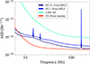 |
Fig. A.1. ASDs adopted in this work for different XG detectors. See Sect. 2.1 and Appendix A for details. |
Table A.1 summarizes the locations, orientations, and chord distances between interferometers of the various detector configurations. Chord distances are calculated assuming the Earth is a perfect sphere with radius R⊕ = 6378.1366 km.
Locations (latitude and longitude), orientations (x-arm azimuth), and chord distances for the different detector configurations considered in this work.
Appendix B: Waveforms and priors
We define spin-aligned, quasi-circular waveforms defined by the parameter set θ = {ℳd, q, DL, dec, ra, θjn, ψ, tgeocent, χ1, χ2, ϕc}, where ℳd, q, and DL denote the detector-frame chirp mass, mass ratio, and luminosity distance, respectively; ra and dec represent the right ascension and declination of the source; θjn denotes the angle between the line of sight and the total angular momentum (J). In the absence of precession, as assumed in this work, J is equal to the orbital angular momentum of the binary (L), and thus θjn corresponds to the inclination angle (ι); ψ is the polarization angle; tgeocent is the coalescence time at the Earth’s center; and ϕc is the phase at coalescence. The waveforms also depend on the aligned-spin parameters χ1 and χ2, defined as χi = ai cos θi, where ai = |χi| is the spin magnitude and θi is the angle with respect to the orbital angular momentum.
We employ frequency-domain waveforms with a reference frequency fixed at fref = 20 Hz (Varma et al. 2022), using the IMRPHENOMXPHM waveform approximant (Pratten et al. 2021; Colleoni et al. 2025), which includes the subdominant modes [(ℓ,|m|) = (2,1),(3,3),(3,2),(4,4)] in addition to the dominant [(ℓ,|m|) = (2,2)] mode. The prior distributions, π(θ), employed in training DINGO are reported in Table B1. In particular, for the detector-frame chirp mass and mass ratio, we chose a prior uniform in primary and secondary masses (Dupletsa 2025); therefore,
 (B.1)
(B.1)
Parameters defining GW signals and their adopted priors.
where ℳd ∈ [40, 1100] M⊙; and
 (B.2)
(B.2)
where q ∈ [0.125, 1]. For the luminosity distance, we chose a prior uniform in comoving volume and source-frame time,
 (B.3)
(B.3)
where DL ∈ [5, 500] Gpc, assuming cosmological parameters as provided by Planck Collaboration VI (2020). For the aligned spin component χi, we form a joint prior as follows:
 (B.4)
(B.4)
where π(ai) = 𝒰(0, 0.9) and cos θi = 𝒰(−1, 1) (Lange et al. 2018; Ashton et al. 2019).
By convention, we set the Earth’s orientation and the positions and orientations of interferometers to those corresponding to the reference time tref = 1126259462.391 s, which coincides with the GPS trigger time of GW150914 (Romero-Shaw et al. 2020). The merger time (tgeocent) of each event was randomly sampled around this reference time. Fixing tref does not entail any loss of generality for short signals, as any time offset can be recovered.
Appendix C: Learning curves and P-P plots
Figure C.1 shows that training and test losses remain consistent across all considered detector configurations, indicating the absence of overfitting. We observe an improvement in the training process compared to Fig. 3 of Santoliquido et al. (2025), where the test losses exhibited significant noise before epoch ∼200.
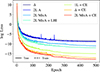 |
Fig. C.1. Log loss as a function of training epochs shown for all detector configurations considered in this study. The solid line represents the training set and the dashed line the test set. See Appendix C for further details. |
Figure C.2 displays the probability–probability (P–P) plots for the different detector configurations. P–P plots are commonly used to assess the reliability of inference algorithms (Cook 2006; Veitch et al. 2015; Talts et al. 2020; Green et al. 2020), by verifying whether the fraction of injected parameters recovered within a given credible interval follows a uniform distribution. This method also enables the computation of p-values for each parameter through a Kolmogorov–Smirnov test. The results reported in Table C.1 show good overall consistency. The plots in Fig. C.2 demonstrate that the improved training procedure produces an unbiased proposal distribution qϕ(θ|d), as evidenced by the curves lying close to a uniform distribution.
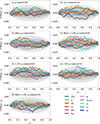 |
Fig. C.2. P–P plots showing the confidence interval (p) on the x-axis versus the difference between the observed fraction of events within that interval and the interval itself (CDF(p)−p) on the y-axis, for each GW parameter. Posteriors are obtained with DINGO (without importance sampling) from 1000 injected BBH signals sampled from the prior (Table B1) for all the considered detector configurations. Shaded regions denote the 1σ, 2σ, and 3σ confidence intervals, with combined p-values shown in the top-left corner of each panel. Individual p-values for each parameter and configuration are reported in Table C.1. See Appendix C for further details. |
p-values (color-coded) for each GW parameter (rows) across different detector configurations (columns).
Appendix D: DINGO-IS versus BILBY
The parameters (θ) of a GW signal are inferred from strain data (d) through Bayes’ theorem (van der Sluys et al. 2008, 2009; Thrane & Talbot 2019; Christensen & Meyer 2022):
 (D.1)
(D.1)
where ℒ(d|θ) is the likelihood function, π(θ) is the prior distribution (see Appendix B) and 𝒵(d) = ∫dθℒ(d|θ)π(θ) is the evidence. Assuming stationary Gaussian noise, the likelihood in Eq. D.1 takes the form (Finn 1992; Veitch et al. 2015; Romano & Cornish 2017; Ashton et al. 2019)
![Mathematical equation: $$ \begin{aligned} \mathcal{L} (d|\theta ) \propto \exp \left[\sum _i \left( (d_i|h_i(\theta )) -\frac{1}{2} (h_i(\theta )\,|\, h_i(\theta ))\right) \right], \end{aligned} $$](/articles/aa/full_html/2026/04/aa58828-25/aa58828-25-eq13.gif) (D.2)
(D.2)
where the index i labels the detectors in the network, hi(θ) denotes the GW signal, and ( ⋅ | ⋅ ) the noise-weighted inner product, defined as
 (D.3)
(D.3)
with Re indicating the real part and * the complex conjugate. The quantity  represents the noise ASD (see Appendix A for details). Equation D.3 is also used to compute the optimal S/N:
 (D.4)
(D.4)
where h(θinj) denotes the GW signal evaluated with injected parameters. For a network of detectors, the total optimal S/N is obtained by adding the individual detector S/Ns in quadrature.
To sample from Eq. D.1, we employed BILBY (Romero-Shaw et al. 2020), a Python library designed for Bayesian inference with the nested sampling algorithm NESSAI (Williams 2021). Thanks to its use of normalizing flows, NESSAI achieves rapid convergence. We fixed the number of live points to n_live = 10_000.
For the source shown in Fig. 2 and observed with the 2L MisA configuration, the default NESSAI settings yield suboptimal performance. To improve robustness, we increased the volume_fraction from 0.95 to 0.98. This parameter controls the fraction of the total probability enclosed by the contour in the latent space—the base space from which samples are initially drawn before being mapped to physical space through the normalizing flow (Williams et al. 2021). Although a higher volume fraction improves performance, it also increases computational cost, which explains the long runtime (∼ 50 hours) required for this source (see Table D.1).
Injected parameters (θinj) of the event shown in Fig. 2, along with the median JSD (⟨JSD⟩, in units of 10−4 nat), which quantifies the deviation between DINGO-IS and BILBY for one-dimensional marginal posteriors.
To quantify the agreement between posterior samples obtained with DINGO-IS and BILBY, we employ the Jensen–Shannon divergence (JSD; Lin 1991), a symmetrized variant of the KL divergence (Kullback & Leibler 1951). The JSD provides a measure of the similarity between two probability distributions, taking values from 0 nat, when the distributions are identical, up to ln(2) = 0.69 nat for completely distinct distributions.
To determine a threshold for the JSD beyond which one-dimensional posteriors can be regarded as statistically different, we follow the procedure outlined in Santoliquido et al. (2025). Using DINGO-IS, we generate 100 independent sets of 105 posterior samples. For each parameter θ, we compute the JSD across all 4950 unique pairs of these sets. Because all samples originate from the same underlying distribution, the resulting JSD values capture statistical fluctuations rather than meaningful discrepancies. We adopt the 95th percentile of these values as the threshold for each parameter (JSDthr in Table D.1). Finally, we compare the one-dimensional posteriors obtained with BILBY to each DINGO-IS set, and verify whether the median JSD lies below the corresponding threshold (⟨JSD⟩ in Table D.1).
Table D.1 lists the JSD values computed for the marginal one-dimensional posteriors of the source analyzed in Fig. 2. The results show that the posteriors obtained with BILBY and DINGO-IS are statistically indistinguishable for both the 2L MisA and 2L MisA + CE configurations. This excellent agreement is further illustrated in Figs. D.1 and D.2, which display the marginalized one- and two-dimensional posteriors for all parameters for the 2L MisA and 2L MisA + CE networks, respectively.
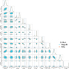 |
Fig. D.1. Marginalized one- and two-dimensional posterior distributions for all parameters for the event shown in Fig. 2 observed with the 2L MisA configuration. Results from DINGO-IS (light blue) are compared with BILBY (orange). Vertical and horizontal lines indicate the true injected values (see Table D.1) and contours represent the 68% and 95% credible regions. See Appendix D for further details. |
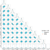 |
Fig. D.2. Marginalized one- and two-dimensional posterior distributions for all parameters of the same event shown in Fig. D.1, this time observed with the 2L MisA + CE configuration. Results from DINGO-IS (light blue) are compared with BILBY (orange). Vertical and horizontal lines indicate the true injected values (see Table D.1) and contours represent the 68% and 95% credible regions. See Appendix D for further details. |
Table D.1 also reports the Bayesian evidence 𝒵(d) defined in Eq. D.1, along with its uncertainty estimated by averaging the weights (Eq. 1) obtained with DINGO-IS (Owen 2013):
 (D.5)
(D.5)
where n denotes the total number of samples drawn from the proposal distribution qϕ(θ|d), and ϵ is the sampling efficiency defined in Eq. 2. The log evidences computed with DINGO-IS and BILBY are consistent within statistical uncertainties.
Appendix E: Information gain
We computed Eq. 3 through a Monte Carlo integration:
 (E.1)
(E.1)
where Ns = 3 × 10⁴ denotes the number of samples drawn from the posterior. In our case, these samples were obtained through sampling-importance resampling (Rubin 1988) based on the importance weights defined in Eq. 1. Using Bayes’ theorem, we can rewrite the ratio inside the logarithm as
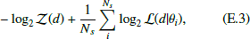 (E.3)
(E.3)
where the log evidence log2𝒵(d) is evaluated through the importance sampling weights (Eq. D.5). We estimated the variance associated with the Monte Carlo estimator of the information gain (Mackay 2003; Talbot & Golomb 2023; Heinzel & Vitale 2025) as follows:
![Mathematical equation: $$ \begin{aligned} \sigma _I^2 = \frac{1}{N_s} \left[ \frac{1}{N_s} \sum _{i=1}^{N_s} \left(-\log _2 \mathcal{Z} (d) + \log _2 \mathcal{L} (d|\theta _i)\right)^2 - I^2 \right], \end{aligned} $$](/articles/aa/full_html/2026/04/aa58828-25/aa58828-25-eq49.gif) (E.4)
(E.4)
where I is defined in Eq. E.2 and σI2 < 10−3 bits for all detector configurations.
Appendix F: Multimodal luminosity distance
We apply Hartigan’s dip test for unimodality (Hartigan & Hartigan 1985; Hartigan 1985) to the one-dimensional marginal posterior of the luminosity distance. A distribution is classified as unimodal if the p-value exceeds 0.01. As shown in Fig. F.1, about 19% (23%) of sources have a multimodal DL posterior for 2L MisA (2L A), while the Δ configurations display only ∼2%.
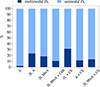 |
Fig. F.1. Percentage of luminosity distance posteriors (y-axis) that are multimodal (dark blue) or unimodal (light blue) for all detector configurations (x-axis). See Appendix F for details. |
Appendix G: Robustness to waveform approximant variations
To assess whether the multimodalities in luminosity distance and sky localization observed in Fig. 2 for the 2L MisA configuration persists under different waveform approximants, we repeat the analysis in zero noise using BILBY (see Appendix D). In addition to the fiducial IMRPHENOMXPHM waveform model (XPHM; Colleoni et al. 2025; see also Appendix B), we both injected and recovered the signals using three additional state-of-the-art inspiral–merger–ringdown (IMR) approximants: NRSUR7DQ4 (Varma et al. 2019), SEOBNRV5PHM (Ramos-Buades et al. 2023), and IMRPHENOMXO4A (Thompson et al. 2024, XO4A).
All considered waveform models describe precessing quasi-circular binaries and include higher-order multipole contributions; however, they adopt distinct modeling strategies (Chatziioannou et al. 2024). In brief, NRSUR7DQ4 is constructed by interpolating numerical-relativity simulations (Field et al. 2014; Blackman et al. 2015) and is therefore typically the most accurate for high-mass systems, such as GW231123 (Abac et al. 2025b; Bini et al. 2026). In contrast, XPHM, SEOBNRV5PHM, and XO4A combine analytical frameworks with numerical-relativity calibration to build complete IMR models that are applicable across the full range of total masses (Buonanno & Damour 1999, 2000; Buonanno et al. 2007; Ajith et al. 2011). The differing modeling strategies and treatments of precession dynamics render these waveform models largely independent. As shown in Fig. G.1, we find no evidence of waveform-induced systematics in the inferred parameters, with all four waveform models reproducing the same number and locations of multimodalities.
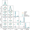 |
Fig. G.1. Marginalized one- and two-dimensional posterior distributions for the detector-frame chirp mass (ℳd), mass ratio (q), luminosity distance (DL), right ascension (ra), and declination (dec) of the event displayed in Fig. 2, observed with the 2L MisA configuration in zero noise. Results from BILBY are presented for different waveform approximants: XPHM (orange), XO4A (grey), NRSUR7DQ4 (teal), and SEOBNRV5PHM (blue). Vertical and horizontal lines indicate the true injected values (see Table D.1) and the contours denote the 95% credible regions. Further details are provided in Appendix G. |
Appendix H: Sky modes in the 2L misaligned configuration
Figure 2 illustrates multimodalities in sky localization for a source observed with the 2L MisA configuration. The presence of these multimodalities is further confirmed in Fig. 4, where almost no sources exhibit a single mode. Most sources (≳60%) display between two and six sky modes, while ∼20% exhibit eight distinct modes.
In this section we provide an intuitive example to illustrate that the presence of multiple sky modes in the 2L MisA configuration is specific to the sources considered in this study, after applying the sample efficiency selection (Sect. 3.1 and the bottom panel of Fig. 1). For a small subset of sources that are excluded from our analysis but still present in the prior space, it is reasonable to expect that the number of sky modes would be significantly lower. Intuitively, the baseline between the 2L ET interferometers becomes effectively long for sources with sufficiently high S/N above a certain frequency threshold, which depends on both the length of baseline and the source’s sky location. A comprehensive study to quantify this effect is beyond the scope of this manuscript and will be addressed in future work.
Figure H.1 shows the one- and two-dimensional marginal distributions obtained with BILBY for two sources at zero noise: a less massive, closer source with ℳdinj = 55.5 M⊙ and DLinj = 6.2 Gpc, with optimal S/N = 87.5, and a more massive, more distant source with ℳdinj = 145.3 M⊙ and DLinj = 37.2 Gpc with optimal S/N = 28.7. The sky location, source-frame chirp mass, mass ratio, and other parameters are fixed for both sources to the maximum-likelihood values estimated for GW250114 (Abac et al. 2025c), while only the luminosity distance—and thus the redshift—are varied. Figure H.1 illustrates that multimodalities in sky localization vanish for the less massive source, whereas they persist for the more massive one, yielding ΔΩ90% = 3 deg2 for the low-mass event and ΔΩ90% = 194 deg2 for the high-mass event.
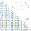 |
Fig. H.1. Marginalized one- and two-dimensional posterior distributions for all parameters, with the exception that this time we show the source-frame chirp mass (ℳs) and redshift (z). The results for the low-mass event (orange) are shown alongside those for the high-mass event (blue). Vertical and horizontal lines indicate the true injected values and contours represent the 68% and 95% credible regions. Top-right panel: Sky map of the low-mass (orange) and high-mass (blue) events, with contours indicating the 50% and 90% credible area. See Appendix H for further details. |
All Tables
Percentage of injections (color-coded) with estimated sky localization errors within the specified areas (columns) for different detector configurations (rows).
Locations (latitude and longitude), orientations (x-arm azimuth), and chord distances for the different detector configurations considered in this work.
p-values (color-coded) for each GW parameter (rows) across different detector configurations (columns).
Injected parameters (θinj) of the event shown in Fig. 2, along with the median JSD (⟨JSD⟩, in units of 10−4 nat), which quantifies the deviation between DINGO-IS and BILBY for one-dimensional marginal posteriors.
All Figures
|
Fig. 1. Top panel: Injections as a function of sample efficiency (ϵ, x-axis) and optimal S/N (ρ, y-axis) for each detector configuration (color-coded). Filled markers indicate injections with sample efficiencies > 1%. Percentages in parentheses denote the fraction of sources with a sample efficiency above 1%, while the horizontal colored lines indicate the median ρ for sources exceeding this threshold. Bottom panel: Injections as a function of detector-frame chirp mass (x-axis) and luminosity distance (left y-axis), with corresponding redshifts (right y-axis). Colored markers indicate events with a sample efficiency greater than 1% in all considered detector configurations. See Sect. 3.1 for details. |
| In the text | |
|
Fig. 2. Top panel: Marginalized one-dimensional posterior distributions for the luminosity distance, recovered with DINGO-IS, for an event observed with the Δ (dark blue) and 2L MisA (light blue) configurations. The results are compared with BILBY (orange). The vertical line marks the injected luminosity distance. The remaining parameters are shown in Appendix D. Middle panel: Posterior samples obtained with DINGO-IS in the Δ configuration for right ascension (ra) and declination (dec), color-coded by luminosity distance. The red cross marks the injected sky position. We also report the sky-localization area (ΔΩ90%) and comoving-volume localization (ΔV90%c) errors. Bottom panel: Same as the middle panel but for the 2L MisA configuration. See Sect. 3.2 for details. |
| In the text | |
|
Fig. 3. Cumulative distributions of events as a function of the information gain (top-left panel; see also Sect. 2.3), the relative variation in luminosity distance (top-right panel; |
| In the text | |
|
Fig. 4. Percentage of sky maps (y-axis) with ΔΩ90% ≤ 100 deg2 exhibiting one to eight or more disconnected modes (color-coded), for all detector configurations (x-axis). See Sect. 3.3 for details. |
| In the text | |
|
Fig. 5. Cumulative distributions of events as a function of the optimal S/N (ρ; Eq. (D.4)), the relative variations in detector-frame chirp mass ( |
| In the text | |
|
Fig. A.1. ASDs adopted in this work for different XG detectors. See Sect. 2.1 and Appendix A for details. |
| In the text | |
|
Fig. C.1. Log loss as a function of training epochs shown for all detector configurations considered in this study. The solid line represents the training set and the dashed line the test set. See Appendix C for further details. |
| In the text | |
|
Fig. C.2. P–P plots showing the confidence interval (p) on the x-axis versus the difference between the observed fraction of events within that interval and the interval itself (CDF(p)−p) on the y-axis, for each GW parameter. Posteriors are obtained with DINGO (without importance sampling) from 1000 injected BBH signals sampled from the prior (Table B1) for all the considered detector configurations. Shaded regions denote the 1σ, 2σ, and 3σ confidence intervals, with combined p-values shown in the top-left corner of each panel. Individual p-values for each parameter and configuration are reported in Table C.1. See Appendix C for further details. |
| In the text | |
|
Fig. D.1. Marginalized one- and two-dimensional posterior distributions for all parameters for the event shown in Fig. 2 observed with the 2L MisA configuration. Results from DINGO-IS (light blue) are compared with BILBY (orange). Vertical and horizontal lines indicate the true injected values (see Table D.1) and contours represent the 68% and 95% credible regions. See Appendix D for further details. |
| In the text | |
|
Fig. D.2. Marginalized one- and two-dimensional posterior distributions for all parameters of the same event shown in Fig. D.1, this time observed with the 2L MisA + CE configuration. Results from DINGO-IS (light blue) are compared with BILBY (orange). Vertical and horizontal lines indicate the true injected values (see Table D.1) and contours represent the 68% and 95% credible regions. See Appendix D for further details. |
| In the text | |
|
Fig. F.1. Percentage of luminosity distance posteriors (y-axis) that are multimodal (dark blue) or unimodal (light blue) for all detector configurations (x-axis). See Appendix F for details. |
| In the text | |
|
Fig. G.1. Marginalized one- and two-dimensional posterior distributions for the detector-frame chirp mass (ℳd), mass ratio (q), luminosity distance (DL), right ascension (ra), and declination (dec) of the event displayed in Fig. 2, observed with the 2L MisA configuration in zero noise. Results from BILBY are presented for different waveform approximants: XPHM (orange), XO4A (grey), NRSUR7DQ4 (teal), and SEOBNRV5PHM (blue). Vertical and horizontal lines indicate the true injected values (see Table D.1) and the contours denote the 95% credible regions. Further details are provided in Appendix G. |
| In the text | |
|
Fig. H.1. Marginalized one- and two-dimensional posterior distributions for all parameters, with the exception that this time we show the source-frame chirp mass (ℳs) and redshift (z). The results for the low-mass event (orange) are shown alongside those for the high-mass event (blue). Vertical and horizontal lines indicate the true injected values and contours represent the 68% and 95% credible regions. Top-right panel: Sky map of the low-mass (orange) and high-mass (blue) events, with contours indicating the 50% and 90% credible area. See Appendix H for further details. |
| In the text | |
Current usage metrics show cumulative count of Article Views (full-text article views including HTML views, PDF and ePub downloads, according to the available data) and Abstracts Views on Vision4Press platform.
Data correspond to usage on the plateform after 2015. The current usage metrics is available 48-96 hours after online publication and is updated daily on week days.
Initial download of the metrics may take a while.