| Issue |
A&A
Volume 709, May 2026
|
|
|---|---|---|
| Article Number | A119 | |
| Number of page(s) | 14 | |
| Section | The Sun and the Heliosphere | |
| DOI | https://doi.org/10.1051/0004-6361/202557024 | |
| Published online | 12 May 2026 | |
Testing spacecraft charging predictions as Parker Solar Probe approaches the Sun
1
Laboratory for Atmospheric and Space Physics, University of Colorado Boulder, 3665 Discovery Drive, Boulder 80303, CO, United States
2
Department of Astrophysical & Planetary Sciences, University of Colorado Boulder, 2000 Colorado Ave, Boulder 80309, CO, United States
3
Department of Physics, University of Colorado Boulder, 2000 Colorado Ave, Boulder 80309, CO, United States
4
Space Sciences Laboratory, University of California, 7 Gauss Way, Berkeley 94720, CA, United States
★ Corresponding author: This email address is being protected from spambots. You need JavaScript enabled to view it.
Received:
28
August
2025
Accepted:
6
March
2026
Abstract
Context. Surface charging must be carefully simulated and predicted for any spacecraft, but especially for those encountering highly variable plasma environments, such as spacecraft near the Sun. Parker Solar Probe (PSP) is a NASA mission that makes in situ solar wind measurements between 9.8 and 155 solar radii (RS). Prior to launch it was predicted that the plasma and photon environment near the closest solar approach would result in large negative spacecraft voltages. Charging of the predicted magnitude (−10 V to −100 V) would significantly modify the measured electron and ion distributions and potentially disturb electric field measurements.
Aims. Multiple surface charging models of PSP that were run prior to launch agreed that PSP should charge negatively as it approaches the Sun. This work aims to compare observational voltage data against pre-launch charging model predictions to investigate the physics of spacecraft charging in near-Sun plasma and photon conditions.
Methods. PSP measurements of spacecraft floating potential are evaluated and compared against pre-launch models. Numerical models and analytic estimates are employed to evaluate how various parameters impact PSP spacecraft surface charging, including variations in the ambient plasma conditions, surface resistance changes brought on by variations in temperature and photoelectron flux, consideration of higher-fidelity spacecraft geometry, and the presence of a second higher-energy population of photoelectrons.
Results. The observed PSP spacecraft floating potential is positive for the majority of each solar encounter at close solar radial distances (R < 25 RS). This directly disagrees with pre-launch simulation predictions. Multiple possibilities for the data-model discrepancy are explored, such as secondary electron emission, surface resistance changes, and photoelectron energy distributions. Simulations reveal that the most effective positive charging mechanism is an enhanced photoelectron yield, which may be caused by a population of higher-energy photoelectrons and lower than predicted plasma densities at perihelion.
Key words: plasmas / space vehicles / space vehicles: instruments / solar wind
© The Authors 2026
 Open Access article, published by EDP Sciences, under the terms of the Creative Commons Attribution License (https://creativecommons.org/licenses/by/4.0), which permits unrestricted use, distribution, and reproduction in any medium, provided the original work is properly cited.
This article is published in open access under the Subscribe to Open model. This email address is being protected from spambots. You need JavaScript enabled to view it. to support open access publication.
1. Introduction
Objects in contact with a plasma, including spacecraft, acquire an electric potential relative to the plasma as a result of charged particles being exchanged between the plasma and the object surface. Understanding and predicting spacecraft charging behavior is important for a wide range of spacecraft engineering applications, including solar panel design and surface material selection (Snyder et al. 1998; Dennison 2015). Spacecraft charging behavior is also critical for the accurate interpretation of in situ fields and particle data. For example, a sufficiently charged spacecraft body will prevent some charged particles from reaching a given detector, while accelerating others toward the detector (Isensee 1977; Maldonado et al. 2023). Spacecraft potential can also be used as a proxy for plasma density, but only when the variability in that potential with respect to ambient plasma parameters is well understood (Pedersen et al. 2008).
For these reasons, detailed spacecraft charging models have been developed, including NASCAP (Mandell et al. 2002) and SPIS (Forest et al. 2001), for scientific and commercial application. The accuracy of these models is tested primarily by comparison with the surface charging of near-Earth spacecraft (Anderson 2012; Yang et al. 2011; Mandell et al. 2002). Therefore, spacecraft sent to regions of space with significantly different plasma conditions present an opportunity to test these models, probing for the possibility of omitted physics.
This study examines the spacecraft charging of the Parker Solar Probe (PSP) spacecraft (Fox et al. 2016). PSP has traveled from ∼215 solar radii, RS (1 AU) to ∼9.8 RS from solar center. With its highly elliptical orbit, PSP encounters a wide range of plasma and environmental conditions, including spacecraft surface temperatures (∼200 K to ∼1800 K), plasma densities (0.1 cm−3 ∼104 cm−3), thermal plasma temperatures (< 1 eV to > 100 eV), and solar photon fluxes (> 500× variation).
This study compares measured PSP spacecraft potential with pre-launch predictions from spacecraft charging models (Ergun et al. 2010; Marchand et al. 2014; Guillemant et al. 2013). Large deviations are identified between model predictions and observations for specific radial distances, suggesting that the charging models did not capture some critical aspect of the system. This study examines possible origins for the data-model discrepancy.
First, secondary electron currents are examined. The magnitude of the secondary electron current on PSP was difficult to constrain prior to launch (Ergun et al. 2010). An analytic estimate for secondary electron current based on PSP observations of the thermal and suprathermal electron populations is compared against the order-of-magnitude secondary electron current required to produce the observed deviations from the modeled spacecraft potential.
Second, the importance of the temperature-dependent conductivity of the PSP heat shield to spacecraft charging is examined. The PSP heat shield has an alumina (Al2O3) coating that faces the sun (Figure 1). The conductivity of alumina varies greatly with temperature (Donegan et al. 2010), an effect that may impact the predicted potential. Although the alumina on PSP has been modeled as both an insulator and a conductor (Donegan et al. 2010; Diaz-Aguado et al. 2021), the bulk resistivity through the layers of the heat shield from alumina to radiator has not been estimated and modeled before. This test is accomplished using SPIS simulation runs, modeled after those used in prior studies (Diaz-Aguado et al. 2021).
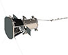 |
Fig. 1. Scale-accurate three-dimensional model of Parker Solar Probe used to highlight the relevant spacecraft geometry. This model includes all spacecraft structures, subsystems, and instruments, but no thermal blanketing or wire harnessing. Fine-scale structures (< 5 cm) are rendered with nonphysical rounded edges. |
Third, previous studies have shown that in sunlit areas of the spacecraft the photoelectron current is overwhelmingly dominant (Ergun et al. 2010; Diaz-Aguado et al. 2021) and that photoelectron production at close approach to the Sun is not well understood (Donegan et al. 2010). Photoemission occurs when photons with sufficient energy liberate electrons from surfaces. Photoelectron yields depend on incident angle and penetration depth of incoming photons, as well as spacecraft surface temperatures. Material properties relevant for photoemission, such as work functions, can vary with temperature (Seely 1941; Rahemi & Li 2015). This study uses SPIS to examine the impact of a reduced work function for alumina due to high temperatures by varying the energy of photoelectrons generated by PSP.
Fourth, previous studies on photoelectron populations in the solar wind suggest that photoelectrons may be more accurately modeled by two populations instead of one (Pedersen 1995; Ergun et al. 2010; Wilson et al. 2023). A higher-energy population of photoelectrons with a peak energy around 10 eV would be able to escape the spacecraft more easily, contributing to a stronger photoelectron current. Including geometric details, such as antenna heat shields, also enhances the estimated photoelectron escape. The effect of adding antenna heat shields to PSP and an additional population of photoelectrons is investigated using a simulation code based on the one used in Marchand et al. (2014).
Finally, the possibility that the PSP plasma wake influences the spacecraft potential observations is examined by comparing the amplitude of wake-related signal perturbations against the magnitude of spacecraft potential deviation from the pre-flight models. PSP travels with a high-velocity relative to the solar wind ion flow, which is expected to produce a strong plasma wake (Ergun et al. 2010). Plasma waves generated by this wake have been observed (Tigik et al. 2022; Malaspina et al. 2022), demonstrating its importance to interpretation of electric field and floating potential data on PSP. Testing these possible origins for the data-model discrepancy limits the possible explanations for why the pre-launch spacecraft charging models did not accurately predict the observed PSP spacecraft charging behavior.
2. Datasets
PSP performs 24 solar encounters during its nominal mission, reducing its perihelion from 35 RS to 9.86 RS using Venus gravity assists (Fox et al. 2016). This study examines the continuous waveform voltage data recorded on the Digital Fields Board (DFB) receiver (Malaspina et al. 2016) as part of the FIELDS instrument suite (Bale et al. 2016) collected over solar encounters 1–23 (10/27/2018–03/22/2023). The voltage data has a sample rate dependent on proximity to the Sun, ranging from ∼1.14 samples/s (DC – ∼1 Hz bandwidth) when PSP is outside of encounter (R > 55 RS), then increasing up to ∼2443 samples/s (DC – ∼2000 Hz bandwidth) when PSP is at closest approach.
PSP is an asymmetric spacecraft, with a long hexagonal bus, a prominent heat shield (sunward directed during close approach), solar panels that can extend out from behind the heat shield, and a long instrument boom in the anti-sunward direction (Figure 1). Most scientific instruments on PSP are mounted on the bus, behind the heat shield, to protect them from the intense solar photon flux. The heat shield is a hexagon prism comprised of multiple layers: two layers of carbon-carbon sandwich approximately 11 cm of carbon foam. The side of the heat shield that faces the Sun is coated in a layer of alumina (Al2O3) to further reflect solar radiation.
There are five voltage probes onboard PSP to measure electric fields between DC and 20 MHz (Bale et al. 2016). Four voltage probes (V1, V2, V3, and V4) are ∼2 m whip antennas mounted nearly orthogonally in pairs in the plane of the heat shield (Figure 1). The fifth voltage probe (V5) is a short rigid antenna, and provides fluctuating electric field measurements along the spacecraft-Sun line. The fifth probe is mounted on the aft instrument boom entirely within the shadow created by the spacecraft heat shield. Consequently, it is often in the spacecraft plasma wake and is not coupled to the plasma via photoelectrons.
PSP’s voltage probes are current-biased, to enable DC electric field measurements. Bias current sweeps are run up to twice per day depending on proximity to the Sun to help determine an appropriate bias current set point. The bias current helps stabilize probe potentials against variability in the thermal plasma environment, by minimizing  (Mozer 2016). The bias currents on PSP are adjusted depending on PSP’s distance to the Sun, to account for the enhanced photoelectron flux close to the Sun.
PSP uses the double probe technique to measure electric potentials and derive electric fields (Bale et al. 2016), using whip antennas as voltage probes. The double probe technique is most successful for voltage probes that are separated from the spacecraft by more than a few Debye lengths (Mozer 2016). Therefore, the measured probe voltages are most independent from the spacecraft body floating potential when the Debye length is comparable or shorter than ∼2 m, the whip antenna length. This occurs close to the Sun (R < 35 RS), when the electron density increases more rapidly with decreasing distance to the Sun than the electron temperature.
The terms “voltage probe” and “antenna” typically refer to significantly different electric field instrument designs (Mozer 2016). PSP is unique in that it uses whip antennas for both high-frequency electric field measurements (> 1 MHz) and DC-coupled electric potential measurements. To simplify the following discussion, the PSP voltage probes are referred to as antennas. In this analysis, the DFB voltage data are taken from the V1, V2, V3, and V4 antennas, each of which measures voltages relative to the spacecraft body potential
 (1)
(1)
for antenna i.
Thermal electron density and electron temperature are determined using quasi-thermal noise (QTN) spectroscopy. On PSP, QTN data are derived by tracking the plasma upper hybrid resonance line in power spectral data, as outlined in Moncuquet et al. (2020).
Ion densities and temperatures are determined from the ion proton moments reported by the Solar Probe ANalyzer for Ions (SPAN-I) instrument (Livi et al. 2022), which is a part of the Solar Wind Electrons, Alphas, and Protons (SWEAP) instrument suite (Kasper et al. 2016). Proton moments are reported a cadence between 0.037 samples/s and 0.2857 samples/s depending on encounter. SPAN-I has field of view limitations caused by the heat shield. SPAN-I proton moment estimates are most reliable when the majority of the proton distribution function is in the instrument’s field of view (Livi et al. 2022). The ability to meet this criterion varies with PSP’s proximity to the Sun.
3. Observations
To compare observations with pre-flight spacecraft charging model predictions, PSP floating spacecraft potential data are examined as a function of radial distance to the Sun. This study focuses on the continuous waveform voltage data recorded by the four antennas in the plane of the heat shield. Data ±10 days from each perihelion were examined, with individual antenna measurements median down-sampled with one-minute windows. Voltage data recording during calibration bias sweeps were removed from consideration. The four antennas measure nearly identical signals, suggesting that wake effects minimally impact the spacecraft floating potential measurement (see Section 4.4).
The spacecraft floating potential (in volts) is defined as
 (2)
(2)
where the V1, V2, V3, and V4 are defined as Vi = Vantenna − Vsc. An offset of +4 V is included to compensate for the floating potentials of the four antennas relative to the ambient plasma. Liu et al. (2024) use calibration bias sweep data and estimated antenna surface photoelectron yields to demonstrate that the antenna floating potential is ≈ + 4 V relative to the ambient plasma for all antennas on all encounters.
A two-dimensional histogram of VSC data as a function of radial distance to the Sun is plotted in Figure 2a. The counts in each radial distance bin were normalized to the maximum count value in that bin. Figure 2b shows the voltage of the maximum count value in each radial bin as a function of solar radial distance (black line). Model predictions for PSP floating potential from Guillemant et al. (2013) (green line), Marchand et al. (2014) (blue star), and Diaz-Aguado et al. (2021) (red line) are overplotted for comparison. Figure 2c indicates the number of one-minute data points in each radial bin. Localized enhancements in Figure 2c correspond to perihelion passes at various radial distances.
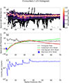 |
Fig. 2. (a) Two-dimensional histogram of the spacecraft floating potential as a function of radial distance (in solar radii, RS) from the Sun. Each radial distance bin of the histogram is normalized by the maximum of its distribution. (b) Voltage corresponding to the peak counts in each radial bin are plotted against radial distance (black). Spacecraft charging model predictions (green, red, blue star) are overplotted for comparison. (c) Number of data samples per radial distance bin of the two-dimensional histogram. |
The solar wind Debye length becomes comparable to or larger than the antenna length at distances > 35 Rs. At these large distances from the Sun, the probe voltage measurements used to determine the spacecraft potential become less independent from the spacecraft body floating potential. However, the primary analysis and conclusions of this study are focused on charging behavior closer to the Sun than 35 Rs, where the floating potential measurements are most accurate.
The value of VSC is positive and increases with decreasing distance to the Sun, demonstrating significant discrepancies between spacecraft charging models and the observations, especially at close approach (9.8 RS). The first step to investigate the source of the data-model discrepancy is to verify whether the spacecraft potential responds to variability in the ambient electron density and temperature in a way that is consistent with prior spacecraft charging studies and theory (e.g., Escoubet et al. 1997; Pedersen et al. 2008 and references therein). Figure 3 tests this idea by plotting scaled electron density (ne) versus VSC.
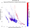 |
Fig. 3. Scaled electron density plotted as a function of spacecraft floating potential (see text for scaling description). The points are color-coded by the thermal electron temperature at the time of each observation. |
If the primary current balance determining spacecraft potential is between thermal electrons and photoelectron current, then ne should be proportional to the photoelectron current density (Jph0), the spacecraft potential, and the photoelectron energy (Vph, in eV), as: ne ∝ Jph0e−Vsc/Vph (Escoubet et al. 1997). As PSP moves toward and away from the Sun, it experiences a large variability in photon flux, and therefore Jph0. To compare the relationship between ne versus VSC across radial distances on the same plot, the measured electron density (nPSP) is scaled by PSP’s radial distance to the Sun (RPSP) as
 (3)
(3)
Here QTN electron densities are used for nPSP, and R0 is taken to be 1 AU. The data in Figure 3 are for PSP solar encounter 19, but all encounters show similar results. Each point is colored by the thermal electron temperature.
Several distinct nscale versus VSC curves are present. These separated curves imply that, while the expected exponential scaling between electron density and spacecraft potential is present, the varying bias current is causing the nscale versus VSC relationship to jump between otherwise quasi-stable states. The bias current is varied depending on the radial distance to the Sun, through a range of 0 μA to −100 μA over an Encounter, causing the nscale versus VSC relationship to shift. A similar effect has been reported in previous studies (Pedersen et al. 2008).
The data in Figure 3 show that the PSP spacecraft potential responds to variation in the thermal electron density in a way that is consistent with prior spacecraft charging studies and theory (Escoubet et al. 1997; Pedersen et al. 2008). Figure 3 shows that both higher electron temperatures and positive spacecraft floating potential values are measured more frequently close to the Sun (R < 25 RS).
4. Discussion
As shown in Figure 2, charging behavior which does not match model predictions is observed on every solar encounter. Instead of charging negatively, as predicted by all pre-launch models (Ergun et al. 2010; Marchand et al. 2014; Guillemant et al. 2013), PSP charges positively at closest approach. The spacecraft floating potential remains around +5 V at large radial distances R > 25 RS, then, around 25 RS, trends positively. This charging trend was not predicted in pre-launch modeling and suggests that there are important physical processes that were not included in the pre-launch modeling.
PSP was predicted to charge negatively at perihelion due to the formation of a nonlinear electrostatic barrier near the heat shield combined with a strong thermal electron current from the solar wind to the spacecraft (Ergun et al. 2010; Marchand et al. 2014). An electrostatic barrier forms near spatially uniform spacecraft surfaces, in the presence of intense solar photon flux, a few Debye lengths away from the surface edges, when the thickness of the photoelectron layer is smaller than the physical extent of the surface (Lphoto < Lsurface). The resulting dense layer of electrons adjacent to the surface creates a negative potential, reflecting electrons back to the surface and reducing photoelectron escape. At PSP’s perihelion, photoelectron loss was predicted to be reduced by 80% (Marchand et al. 2014).
Another physical driver of the negative charging observed in modeling is the ion wake. The relative velocity between the spacecraft and the solar wind plasma is higher than the thermal velocity of the solar wind ions, therefore a wake forms behind the spacecraft, mostly devoid of solar wind ions. The negative potential of this wake structure should further reduce electron escape from the spacecraft in the direction of the wake, leading to an even more negative spacecraft potential. The large negative potential well behind PSP due to its wake was modeled in Ergun et al. (2010).
These two physical phenomena were predicted to be the primary physical drivers for the negative spacecraft floating potential modeled at closest approach. However, as shown in Figure 2, this negative charging behavior is not consistently observed at perihelion. As PSP makes its closest approach at 9.8 RS, the spacecraft floating potential commonly reaches ≈+10 V.
There are two possible explanations for why the spacecraft charges positively at close approach rather than negatively. Either the true solar wind plasma conditions are significantly different than those used in the pre-flight modeling, or the spacecraft surface interactions with the solar wind plasma and solar photons were not fully captured by the pre-flight models.
4.1. Analytic estimates
The first physical explanation investigated is underestimation of secondary electron emission. Secondary electrons are created when an energetic electron or ion strikes the surface of a spacecraft and causes the emission of one or more electrons, causing the spacecraft to charge positively.
The efficacy of this process depends on the material that the electron strikes and the energy of the incoming particle. The effectiveness of secondary emission via ions is thought to be 50% (Garrett 1981), making the secondary current from this source essentially equal to half the ion current, and therefore a negligible contribution to the overall charging behavior (Ergun et al. 2010).
Electrons can eject other electrons from the spacecraft surface if they have sufficient energy. The secondary electron yield varies significantly across material. For example, the Niobium-C103 used on the antennas can eject multiple electrons with just a 30 eV electron strike, whereas the alumina on the heat shield may require an electron strike up to 200 eV (Diaz-Aguado et al. 2020). Since the energies of electrons in the solar wind vary significantly, an incoming electron can liberate no electrons, or up to five or six per strike, depending on incoming energy. Prior experiments estimating PSP secondary electron yields did not use materials consistent with the as-flown PSP spacecraft (Figs. 1 and 4, Donegan et al. 2010). Thus, it is possible that the secondary electron yield estimates were underestimated in pre-flight spacecraft charging models, which based their secondary electron yields on Donegan et al. (2010).
Secondary electron yields can also be effected by surface contamination, possibly leading to further variation from prior estimates. However, this was not explored in the current study.
The secondary electron yield for alumina was found to be four at an incident energy of 200 eV, as shown in Figure 4 of Donegan et al. (2010). As PSP approaches the Sun, an increasing portion of the thermal electron population from the solar wind can be energetic enough to generate secondary electrons. If this charging mechanism was underestimated, the models could be missing a significant positive current.
To examine the viability of this explanation, an analytic code is employed that solves the spacecraft charging equation:
 (4)
(4)
Equation terms are defined following (Ergun et al. 2010), where ϕ is the spacecraft potential, and Ix describes currents due to photoelectrons, thermal electrons, secondary electrons, protons, and the applied bias current.
This equation is solved for a simplified geometrical model of PSP, comprised of the sum of surface areas from two cylinders (one for the spacecraft main bus, one for the heat shield) and a truncated cone representing the spacecraft thermal radiators. The truncated cone did not include flat circular caps to the shape, to better mimic PSP’s radiator geometry. The total external surface area of this geometry is 25.3 m2. The total external surface area of PSP is not precisely known because the addition of multilayer insulation (MLI) over the spacecraft bus increases the surface area beyond estimates based on spacecraft mechanical drawings. Therefore this approximation is used. Solar wind particle densities and temperatures were taken from the QTN electron data and the SPAN-I proton data as median values of data recorded in 0.1 RS windows around desired radial distances.
The spacecraft potential is solved for over a range of radial distances between 32 RS and 9.8 RS. Plasma parameters used as input to the analytic equation are outlined in Table 1. Since this equation is only expected to be accurate to order-of-magnitude, SPAN-I plasma moments were used for all radial distances despite field-of-view limitations.
Plasma parameters used in analytic estimate.
To estimate the secondary electron current, equations given by Diaz-Aguado et al. (2020) were used, specifically equations A.2 and A.6 which quantify the secondary emission efficiency and the output energy. Both the electron core distribution and the electron strahl distribution were included in the analytic estimate.
The density of the electron strahl population is estimated from previous solar wind studies (Halekas et al. 2020; Abraham et al. 2022), which find that the strahl population of electrons close to the Sun should be about 1−2% of the core density. Our model estimated the strahl density to be 2% of the observed QTN electron density, since only order-of-magnitude estimates were desired.
The electron distribution function for the strahl population is modeled as
 (5)
(5)
where ne, s is the density of the strahl electrons, and vth, ∥ and vth, ⊥ are the thermal velocities of the strahl electrons in the parallel and perpendicular directions:  ,
,  . The velocities of the strahl electrons in the parallel and perpendicular directions are v∥ = vpar − upar, vpar, v⊥, 1, and v⊥, 2. upar is the bulk velocity of the strahl electrons, defined as
  , where Es, peak is defined as 200 eV for all radial distances.
To estimate the secondary electron current emitted from the surface of PSP, the effectiveness of the emission with respect to impact angle and incident energy must be quantified. The output energy distribution of the emitted secondary electrons is also important. The output distribution used for the analytic calculation is from Diaz-Aguado et al. (2020):
![Mathematical equation: $$ \begin{aligned} g_{\rm SE}(E_{\rm SE}) = \left\{ \frac{6 * \frac{E_{\rm SE}}{\Phi }}{[1+\frac{E_{\rm SE}}{\Phi }]^4}\right\} . \end{aligned} $$](/articles/aa/full_html/2026/05/aa57024-25/aa57024-25-eq10.gif) (6)
(6)
Here Φ represents the work function and ESE represents the energy of the emitted secondary electrons. The distribution typically peaks between 1−3 eV (Hoffmann 2010; Diaz-Aguado et al. 2020).
The following equation for emission efficiency from (Hoffmann 2010; Diaz-Aguado et al. 2020) is also used:
![Mathematical equation: $$ \begin{aligned} \delta (E) = \frac{\delta _{\rm max}}{[1-e^{-r_{\rm max}}]}\left(\frac{E}{E_{\rm max}}\right)^{1-n}[1-e^{-r_{\rm max}(\frac{E}{E_{\rm max}})^{n-m}}]. \end{aligned} $$](/articles/aa/full_html/2026/05/aa57024-25/aa57024-25-eq11.gif) (7)
(7)
Here E is the incident electron energy, defined as
 (8)
(8)
The δmax is the maximum secondary electron yield for the material, which is approximated for the spacecraft using the value for unannealed tungsten, as the value for germanium black Kapton, used as the upper layer of the spacecraft body MLI, was not available. The maximum secondary electron yield for unannealed tungsten is 1.5 ± 0.1 electrons per incident electron. The Emax is the incident electron energy at maximum secondary electron yield, which is 276 eV for unannealed tungsten. n and m are power law coefficients that correspond to the slope of log–log plots of the secondary electron yield (Wood et al. 2019), with n being the slope of the function below maximum yield and m being the slope of the function above maximum yield. The fitting parameter, rmax, is entirely determined by n, m, and Emax, and determined by the normalization of the fitting function. Details for all variables are outlined in Diaz-Aguado et al. (2020).
Using the above definitions, the secondary electron current density due to the strahl electrons is
 (9)
(9)
The secondary electron current due to the core solar wind electron distribution is calculated similarly, as outlined in the Appendix. The total secondary electron current density is given by jse, tot = jse, s + jse, c, where jse, c is the secondary electron current density due to the core solar wind electron distribution.
These equations provide an order of magnitude estimate for the secondary electron current throughout PSP’s orbit. The calculated secondary electron current can then be scaled arbitrarily within Equation (4) to determine how large it would need to be in order to recreate the positive charging trend observed.
The results of the analytic calculation are shown in Table 2. The secondary current scaling needed to replicate the observed charging trend at various radial distances is included in the bottom row. The secondary current may be a plausible explanation R > 25 RS. However, the secondary electron current must be increased by 10x to 40x over physically reasonable estimates to replicate the observed positive charging close to the Sun. Based on these results, it is unlikely that inaccuracies in secondary electron current modeling are sufficient to explain the model-data discrepancy.
Results from analytic estimate at each simulated radial distance.
4.2. SPIS modeling
The alumina-coated side of the heat shield is the largest photoelectron producing surface on PSP. However, alumina is not a conductor, and its conductivity varies considerably in the PSP environment. This creates uncertainty in how well the photocurrents associated with the heat shield couple to the rest of the spacecraft bus.
The resistance of alumina is dependent on temperature (Donegan et al. 2010). As PSP approaches the Sun, the resistance of the alumina is expected to drop ten orders of magnitude, causing a significant change in electrical conductivity on a large surface of the spacecraft (Donegan et al. 2010).
Additionally, since the photoelectron current should dominate all other currents on PSP sunlit surfaces, an underestimation of the photoelectron yield would produce an inaccurately modeled spacecraft potential. Further, photoelectron yield can be extremely variable across material, temperature, radiation conditions, and incident angles of incoming photons (Donegan et al. 2010). It is possible that this current contribution was underestimated in previous models (Ergun et al. 2010; Marchand et al. 2014; Diaz-Aguado et al. 2021).
The Spacecraft Plasma Interaction System (SPIS) code is used to explore how assumptions about the conductivity of alumina and photoelectrons impact charging model predictions. SPIS is a three-dimensional particle-in-cell code that takes spacecraft geometry, surface conductivity, and ambient plasma properties as inputs, then self-consistently solves the Vlasov-Poisson equations for the spacecraft floating potential.
This study uses a simplified geometrical model of PSP as defined in prior study (Diaz-Aguado et al. 2021). At the time of the prior study, PSP had only passed within 35 RS of solar center. Now, solar wind data exists as close as 9.8 RS and can be incorporated into the model. The PSP geometry and model mesh are shown in Figure 4.
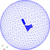 |
Fig. 4. Spacecraft geometry and mesh used for the SPIS model. The geometry is from Diaz-Aguado et al. (2021). The heat shield and singular FIELDS antenna are not connected to the spacecraft bus due to mesh convergence errors. |
The following cases were defined to investigate the role of heat shield resistivity in the observed positive charging. All cases were modeled using plasma parameters relevant to 9.8 RS. (Case 1) Assume that the heat shield is fully insulated from the spacecraft body (1.4 × 10⁹ Ohms). (Case 2) Assume that the total resistance between the heat shield and spacecraft body is 14.1 MOhms. (Case 3) Assume that the total resistance between the heat shield and spacecraft body is 14.1 Ohms. (Case 4) Assume that the total resistance between the heat shield and spacecraft body is 0.00143 Ohms. A summary of the simulation cases is included in Table 3 for reference.
Description for Cases 1−4 and the resulting spacecraft floating potential.
In each case, SPIS treats the heat shield and the spacecraft bus as two separate electrical nodes. Resistance between the heat shield and the spacecraft bus is estimated by modeling the heat shield layers as resistors in series and determining the through resistance from the front of the heat shield to the spacecraft body. The resistance is calculated as
 (10)
(10)
where RAlO3 is the resistance of alumina, RC − C is the resistance of carbon-carbon, and Rfoam is the resistance of carbon foam.
The alumina resistances for Cases 3 and 4 are determined empirically over temperatures ranging from 875 K to 1350 K (Donegan et al. 2010). Resistivities corresponding to 0.08 AU (17 RS) and 0.05 AU (10.8 RS) were selected, 105Ω-m and 10Ω-m, respectively. The alumina resistance for Case 2 was selected arbitrarily as a data point to bridge Case 1 and Cases 3 and 4. The resistance for the carbon-carbon and the carbon foam layers were kept constant for all cases. The resistivity of carbon-carbon is approximated using the resistivity of graphite (9.8 × 10⁻⁶Ω-m, Powell & Childs 1972), since the value for carbon-carbon was not available. The resistivity of carbon foam, 7 × 10⁻⁴Ω-m, was taken from the carbon foam manufacturer who supplied the PSP heat shield material (Ultramet 1990). The plasma parameters were held fixed at the 9.8 RS values while the resistivity was changed to isolate the effect of varying the resistance on the spacecraft floating potential.
A fifth SPIS simulation case is defined to determine how the energy of photoelectrons generated at the heat shield may contribute to the observed positive charging (Salem et al. 2023). Case 5 systematically increases the escape energy of liberated photoelectrons to observe the effect on the spacecraft floating potential.
Case 5 investigates the impact of varying the energy of photoelectrons created on the alumina-coated surface of the heat shield. As PSP approaches the Sun, the temperature on the heat shield of the spacecraft is estimated to increase to temperatures upwards of 2000°C. The work function of metals has been observed to decrease slightly at high temperatures (Seely 1941), due to the thermal expansion of the material’s crystal lattice (Kiejna 1986). The thermal expansion separates electrons from the metal’s nuclei, reducing the energy barrier necessary for electron liberation. A reduction in work function for a material results in a higher energy of liberated photoelectrons, due to the conservation of energy. By systematically increasing the energy of the liberated photoelectrons, Case 5 investigates the impact a reduced work function of alumina has on the spacecraft floating potential.
Solar spectrum variability related to the solar cycle was not considered in previous modeling (Ergun et al. 2010; Marchand et al. 2014; Diaz-Aguado et al. 2021). Prior studies showed that solar cycle variability can lead to changes in solar irradiance at wavelengths relevant for photoelectron production (Sternovsky et al. 2008). Higher-energy (∼10 eV) photoelectron fluxes have been shown to be affected by solar cycle at 1 AU (Wilson et al. 2023). Since the PSP nominal mission spanned solar minimum to solar maximum, it is possible that higher-energy photoelectron fluxes are increasing with solar cycle on PSP.
Prior studies assume that heat shield photoelectrons should have an energy of ∼2 eV, but energies up to ∼3 eV are possible (Diaz-Aguado et al. 2020). Prior studies predicted that photoelectrons generated on the heat shield would form an electrostatic barrier (Ergun et al. 2010; Marchand et al. 2014). The properties of this barrier may vary if the energy of liberated photoelectrons is changed due to a reduced work function for alumina or some solar cycle variability.
Finally, to quantify the impact of the assumptions made in each of these cases, a baseline case was run. The baseline case uses QTN plasma parameters with 3770 cm−3 for electron density and 76.8 eV for electron temperature. Proton density is assumed to be equal to the electron density. A proton temperature of 92.7 eV is used, determined from SPAN-I moments. The electron density used here is approximately a factor of two less than was assumed in prior PSP close-approach modeling studies (Ergun et al. 2010; Marchand et al. 2014; Diaz-Aguado et al. 2021). These plasma parameter values were determined by taking the median of the distribution of all available data recorded within 0.1 RS of 9.8 RS. A magnetic field of 2106 nT in the radial direction is also utilized.
Prior SPIS modeling results at 9.8 RS (Diaz-Aguado et al. 2021) were successfully replicated using SPIS version (6.1) and the geometry provided in Diaz-Aguado et al. (2021).
The baseline case, with updated solar wind temperatures and densities, produces a spacecraft floating potential of −11 V at 9.8 RS, similar to prior modeling (Ergun et al. 2010; Marchand et al. 2014; Diaz-Aguado et al. 2021). Therefore, differences between measured and previously assumed close-approach solar wind parameters alone are not sufficient to explain the observed positive charging.
Case 1 results in a floating potential of −19 V. Case 1 assumes that the sun-facing surface of the heat shield is electrically isolated from the spacecraft bus. Under these simulation conditions, the shadowed surfaces of the spacecraft are dominated by the thermal electron current, producing a significantly negative spacecraft floating potential.
As described earlier in this section, Cases 2, 3, and 4 test the influence of varying the resistivity of alumina between 14.1 MOhms and 0.00143 Ohms. Case 2 and Case 3 produce spacecraft floating potential values of −18 V and −12 V, respectively. Case 4 results in a spacecraft floating potential of −12 V. The simulated voltages for Cases 1 and 2 and for Cases 3 and 4 differ by less than a volt. When resistance between the heat shield and the rest of the spacecraft bus drops significantly due to changes in temperature, the spacecraft bus potential becomes more strongly influenced by photoemission. This effect is expected to become more significant as PSP approaches the Sun, as the heat shield gets hotter, decreasing the alumina resistance (Donegan et al. 2010; Diaz-Aguado et al. 2021).
Case 5 produces spacecraft potentials closer to positive as photoelectron energies are increased (Table 4), because more photoelectrons are able to escape the spacecraft. The baseline case assumes that the peak of the emitted photoelectron Maxwellian distribution is 2 eV. When the peak of the Maxwellian is increased to 4 eV or higher, the spacecraft floating potential reaches ∼ − 3.2 V. While none of the Case 5 simulated potentials are positive, they are more positive than the outcomes of other SPIS runs.
Case 5 Results at 9.8 RS.
The increase in photoelectron energy is the only simulated physical change that results in a significantly more positive floating potential compared to the baseline SPIS case. Increasing the photoelectron energy past 4 eV has no significant effect on the simulated spacecraft voltages.
To investigate this result, the simulated position-dependent volume potentials at 9.8 RS were plotted for two different simulated photoelectron energies. The first simulation plotted was the SPIS baseline case, which models photoelectron temperatures as 2 eV. The second simulation plotted maintains the same plasma conditions as the baseline case, but increases the photoelectron temperatures simulated to 14 eV. The output of these simulations contains the volume potential around the spacecraft, including the potential well due to the electrostatic barrier in front of the spacecraft heat shield along with the potential well due to the ion wake behind the spacecraft. Each of these volume potentials is sliced first along the spacecraft-Sun plane, then along the spacecraft-Sun line, as shown by the black dashed line in Figure 5a.
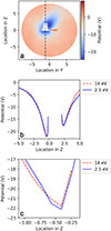 |
Fig. 5. (a) Volume plasma potential sliced along the spacecraft–Sun line in V for PSP at 9.8 RS when photoelectron temperatures are simulated as 14 eV. Dark blue represents areas of negative potential around the spacecraft, while red represents areas of positive potential. The electrostatic barrier is present in front of the heat shield and the ion wake is present behind the spacecraft in the anti-RAM direction. (b) Plasma potential along the black dashed vector shown in the top panel plotted for the simulated photoelectron temperatures of 2 eV (blue line, baseline case) and 14 eV (red line, high-end limit). The electrostatic barrier in front of the spacecraft is located at ∼−0.4 m. The potential well dips to −22.3 V for the baseline case and −21.7 V for the high-end limit case. The spacecraft floating potential itself is not included in the plot data, creating a gap in the plotted potential from ∼0 m to ∼2.4 m. (c) Zoomed-in view of the potential well at ∼−0.4 m in front of the spacecraft. |
The output of the slice is plotted in Figure 5b, where the blue line represents the potential along the black vector of the 2 eV photoelectron temperature baseline case and the red line represents the potential along the black line of the 14 eV high-end limit photoelectron temperature case. A zoomed-in view of the electrostatic barrier in front of the spacecraft heat shield (∼−0.4 m) is shown in Figure 5c. The electrostatic barrier becomes shallower (more positive) when the photoelectron energies increase. This implies that if the alumina’s work function reduces with the thermal expansion of the material, the potential surrounding the spacecraft becomes more positive. However, this mechanism alone cannot be responsible for the observed positive charging, as the simulated spacecraft remains negative at close approach.
4.3. Numerical simulation
4.3.1. Updated spacecraft, updated solar wind conditions, high-energy photoelectron tail
As discussed previously, an electrostatic barrier forms near spatially uniform spacecraft surfaces, a few Debye lengths away from the surface edges, when the thickness of the photoelectron layer is smaller than the physical extent of the surface. Photoelectron escape on PSP is enhanced on surfaces where the conditions of electrostatic barrier formation are not met. For example, these conditions are broken at the edges of the PSP primary heat shield and on the antenna heat shields. Adding geometric detail to photoemitting surfaces in models is therefore expected to result in a larger photoelectron current because weaker electrostatic barriers form on these features.
The PSP heat shield satisfies the above barrier conditions when near the Sun (R < 20 RS). It is a large (∼2.3 m diameter), spatially uniform surface exposed to the Sun. The electrostatic barrier thickness is related to the Debye length in the photoelectron layer (lDph). The layer thickness is roughly several lDph and depends on the photoelectron yield and intensity of sunlight. Under a relatively high yield, Jph0 is expected to be 16 mA/m2 at ∼9 RS, and the thickness of the electrostatic layer is on the order of 10 to 25 cm, which is significantly smaller than the PSP heat shield. Prior simulations showed that photoelectron escape is expected to be considerably higher at the edges of the primary heat shield (Ergun et al. 2010).
Photoelectrons in the solar wind are often modeled by single, isotropic Maxwell-Boltzmann distributions (Halekas et al. 2020). However, there is evidence to suggest that photoelectrons are more accurately represented by two populations: a primary population with a peak energy around 2 eV and a secondary population with a peak energy around 10 eV (Pedersen 1995; Ergun et al. 2010; Wilson et al. 2023). Most primary population photoelectrons have too little energy to escape to space through the electrostatic barrier (see Section 4). Most photoelectrons from the secondary higher-energy population will be energetic enough to penetrate the barrier and leave the spacecraft. These escaping photoelectrons may contribute significantly to the photoelectron current driving the spacecraft positive near perihelion.
There are several important disparities in the pre-flight simulations compared to the true PSP spacecraft and measured plasma conditions. The spacecraft geometry used in the Marchand et al. (2014) study, for example, used a 1 m2 shield whereas the PSP heat shield is closer to 4 m2. PSP, as launched, has four small heat shields at the base of the electric field antennas in the plane of the heat shield (Bale et al. 2016). These surfaces are exposed to direct sunlight, but were not included in prior modeling work. The pre-flight estimated plasma conditions had density and electron temperatures significantly different from what PSP commonly encounters. Importantly, the Marchand et al. (2014) study did not include a high-energy photoelectron population (Pedersen 1995; Ergun et al. 2010). It is important to mention that SPIS does not allow for more than one population of photoelectrons, making the addition of this physics impossible in the simulations discussed earlier in this study.
A new PSP simulation based on the modeling code used in the simulation from Marchand et al. (2014) is run, with several changes. The primary changes are an increase in the primary heat shield size, the addition of antenna heat shields, reduced simulation grid spacing, and solar wind parameters representative of those measured by PSP.
The shield size is increased to a 2.3 m diameter circle, and the heat shields for the electric field antennas are added; they are sized as 2.5 cm × 2.5 cm × 25 cm (see Figure 6, top). The simulation grid spacing is reduced to 2.5 cm to better model the photoelectron density and electrostatic barrier. The spacecraft body and magnetometer boom are modified to conform better with the in-flight PSP geometry. As in Marchand et al. (2014), many fine geometric details of the spacecraft bus behind the heat shield are not included; it was shown that such fine details did not dramatically alter the spacecraft potential in simulations (Marchand et al. 2014).
 |
Fig. 6. Spacecraft floating potential from the baseline numerical simulation. The heat shield is circular with a 2.3 m diameter and includes four small heat shields over the electric field antennas (top). The potential minimum to the lower left of PSP is due to the ion wake. The potential minimum just above the heat shield is the electrostatic barrier. |
To begin, a baseline simulation is run with the solar wind parameters listed in Table 5. The primary changes from Marchand et al. (2014) include a lower average solar wind density, as observed, with nSW = 4000 cm3, a lower electron temperature (Te = 50 eV), and a 10 eV photoelectron population corresponding to 5% of all photoelectrons produced (Pedersen 1995; Ergun et al. 2010; Wilson et al. 2023).
Baseline numerical simulation parameters.
The updated baseline simulation (Figure 6) results in a −1.10 V spacecraft floating potential, which is higher than those predicted in the Marchand et al. (2014) study (−5 V) for nSW = 4000 cm3. Figure 6 (bottom) displays the electric potential in the X − Y plane at Z = 0. The X direction is toward the Sun, the Y direction is the orbital direction of PSP, and the Z direction is normal to the orbital plane.
Figure 7 displays the ion and electron densities using the same format. The ion density (Figure 7a) has a deep ion wake due to the combination of the solar wind speed and orbital motion of PSP, the latter of which can reach 195 km/s at perihelion. The ion vacuum in the wake creates a deep negative potential seen in the lower left of Figure 6. The electron density is broken into three parts. Figure 7b displays the thermal electron density from the ambient solar wind, where depletions in the thermal electron density are visible in the ion wake and above the heat shield. These features are consistent with the potential wells modeled using SPIS from Section 4.2 (Figure 5).
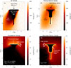 |
Fig. 7. Ion and electron densities from the baseline simulation. (a) Solar wind ion density. (b) Solar wind thermal electron density. (c) Photoelectron density. (d) Secondary electron density. |
Figure 7c displays the photoelectron density, and Figure 7d displays the secondary electron density, both on a logarithmic scales. The thin photoelectron layer just above the heat shield (white area in Figure 7c) is responsible for the negative electrostatic barrier seen in Figure 6. Few low-energy photoelectrons can penetrate the electrostatic barrier above the heat shield; escape of the low-energy photoelectrons is primarily from the edges. The high-energy photoelectrons, those above 10 eV (the electrostatic barrier depth), can directly escape. Without the high-energy photoelectron population, fewer photoelectrons would escape in the +X direction. Secondary electron edge escape is visible in Figure 7d, as few secondary electrons escape directly from the center of the heat shield but instead escape from the edge of the shield where the electrostatic barrier is lower. A lower-amplitude electrostatic barrier around the spacecraft below the heat shield is formed by the secondary electrons.
4.3.2. Sensitivity to parameters
To better understand how spacecraft floating potential depends on individual parameters, the baseline simulation in Figures 6 and 7 is rerun with parameter changes. The results are summarized in Figure 8 and Table 6. The basic principle that governs the spacecraft floating potential is the balance of currents. Here, four primary currents are considered. The thermal electron current (Itherm, e) to the spacecraft is the only negative current. The ion (Ii), photoelectron (Iphoto), and secondary electron (Ise) currents are positive. Current balance requires
 (11)
(11)
Sensitivity of VSC to changes in parameters.
Figure 8 displays the modeled spacecraft floating potential when the plasma density (nSW) is varied from 1000/cm3 to 9000/cm3. As expected, nSW has a strong influence on spacecraft floating potential. Higher nSW results in a strong (negative) Itherm, e, which cannot be offset by Iphoto and Ise currents if VSC > 0 due to the electrostatic barrier. Ii is largely insensitive to spacecraft floating potential and stays roughly ∼0.1 Itherm, e (∼1 mA in Figure 7a).
Interestingly, reducing nSW has a strong effect on spacecraft floating potential. The high-energy (10 eV) contribution of Iphoto is less sensitive to spacecraft floating potential than nSW. Thus, if nSW is reduced such that Itherm, e is less than the high-energy part of Iphoto, the spacecraft floating potential must increase to roughly +10 V to reduce Iphoto. Figure 8 shows a steep increase in spacecraft floating potential at low nSW.
To test the influence of the high-energy component of Iphoto on the spacecraft floating potential, two more simulations are run; one with no 10 eV photoelectron population (0%) and one where the 10 eV population is 10% of all photoelectrons. The results in Table 6 show a strong nonlinear sensitivity of spacecraft floating potential to the high-energy population. For the 0% case, the spacecraft floating potential changes by approximately −5 V relative to the baseline simulation. For the 10% case, the increase is smaller (∼3 V). This nonlinearity is also evident in Figure 8.
While the high-energy component of photoelectrons has been constrained by observation (Pedersen 1995), the energy distribution of secondary electrons and the net yields are largely unknown. The value of Ise (1.46 mA) is lower than Iphoto (7.12 mA) in the baseline simulation (see Figure 6), but a high-energy component or a higher production efficiency of secondary electrons could have a significant effect.
The solar wind electron temperature (Te) has several paths to impact VSC. The current, Itherm, e, is proportional to  , so a high Te forces Itherm, e more negative. The value of Te also influences the depth of the electrostatic barrier and ion wake potential (e.g., Figure 6), which effects Iphoto and Ise. A high Te increases the depth of the electrostatic barrier and the ion wake (less shielding), which decrease Iphoto and Ise. These impacts combine in the model. Reducing Te from 85 eV (simulated in prior works) to 50 eV (closed to typical measured values) increases VSC by ∼7 V. Thus, the earlier simulations that used Te = 85 eV as a baseline showed more negative VSC (Ergun et al. 2010; Marchand et al. 2014).
The geometric changes to the simulated spacecraft may also influence VSC. It was shown in Ergun et al. (2010) that a 1/4 scale model of the PSP spacecraft resulted in a higher VSC. Thus, one might have expected the increased size of PSP in the baseline simulation should have resulted in a more negative VSC. This increase appears to have been offset by the addition of the electric field heat shields. These four small heat shields (Figure 6) have direct exposure to sunlight and, even though they have a small area, their photoelectron escape efficiency is high. Table 6 shows a ∼3 V decrease in VSC when the electric field heat shields are removed.
4.3.3. Conclusions from updated simulations
The two most significant changes from prior simulations that can partly reconcile VSC derived from simulations with the observed VSC are the lower average values of nSW and Te compared to pre-flight estimates and that the simulations in Marchand et al. (2014) did not include an additional, higher-energy population of photoelectrons. The increased physical size of of the spacecraft and the addition of the electric field heat shields were shown to have opposing effects of similar magnitude; the larger heat shield causes VSC to be more negative whereas the electric field heat shields increased Iphoto, which drives VSC more positive.
The observations (e.g., Figure 3) demonstrate that VSC is sensitive to nSW and Te as insinuated by the simulations, placing the current simulations in qualitative agreement with the PSP observations, but some discrepancies remain. The secondary electron energy distribution and production rate is the least well understood of the simulation parameters. An energetic component of the secondary electrons could significantly alter Ise and thus change VSC. Lastly, the impact of a magnetic field on VSC is not fully studied. A 2 eV electron has a gyroradius of ∼3 m in a ∼1000 nT field so Ii and Itherm, e are not expected to be measurably impacted by a magnetic field, but Ise and Iphoto may have small changes.
4.4. Influence of the ion wake
Near closest approach, the PSP spacecraft velocity (∼180 km/s) approaches that of the solar wind (∼200 km/s). Therefore, PSP’s ion wake does not form directly behind the spacecraft, but rather diagonally behind it (Ergun et al. 2010). In this geometry, electric potential gradients generated by the wake may influence spacecraft potential measurements made by the antennas closest to the wake. Because the spacecraft potential is determined using the average of all four antennas in the plane of the heat shield, it is possible that the presence of the wake could bias the observed spacecraft potential.
To quantify this effect, the variance in electric potential measured by the four antennas is calculated. The calculation method examines the population variance of the potential data, defined as
 (12)
(12)
where Vi(t) represents the measured potential by each antenna at a time t. ⟨V1, 2, 3, 4⟩ is the average of all four antenna-measured potentials calculated in a given one-hour window, and N is the number of samples of measured antenna potential data in that window.
The value of Varp remains less than 1 V for most of each encounter, as shown for Encounter 23 in Figure 9. It increases as PSP approaches the Sun, reaching as high as ∼2 V on each encounter. The maximum Varp is ∼10−15% of the measured spacecraft floating potential within 25 RS and ≪10% for larger radial distances.
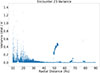 |
Fig. 9. Variance (Varp) calculated for Encounter 23. For most of each encounter, the variance remains small, less than 1 V. Each encounter has an average maximum (Varp) of approximately 2 V at closest approach, which is ∼10−15% of the measured spacecraft floating potential value. Features in the variance from 50 RS − 55 RS are likely due to the instrument mode transitioning from out-of-encounter to in-encounter. |
The observed variances demonstrate that the antennas do measure asymmetric potentials, likely due to the ion wake. However, the variance is small compared to the overall potential at all radial distances. Therefore, averaging over all four antennas is still an accurate representation of the spacecraft floating potential with respect to antenna asymmetries.
5. Results
A significant model-data discrepancy is demonstrated on PSP as the spacecraft approaches the Sun. While spacecraft charging models predicted significant negative spacecraft potentials, strongly positive potentials are observed. Five possible explanations were examined.
The first possible explanation is underestimation of secondary electron emission in spacecraft charging models. Secondary electron emission is found to be an unlikely candidate to explain the model-data discrepancy. Analytic estimates show that, at closest approach, the secondary electron current would need to be 43x higher than observed to replicate observed positive charging. This implies that every incoming particle striking the surface of the spacecraft would need to eject ∼43 electrons. While up to five secondary electrons can be liberated by single impacts (Ergun et al. 2010; Donegan et al. 2010), 43 is not physically reasonable.
A caveat to this analysis is that the PSP geometry used in the analytic estimates is highly simplified, and does not include features on the spacecraft that may impact electron loss (e.g., antennas, magnetometer boom). Another caveat is that the estimated secondary electron current was calculated using empirical parameters, such as rmax, whose origins are not well documented (Lundgreen & Dennison 2020).
The second possible explanation is a misrepresentation of alumina resistivity in prior spacecraft charging studies (Donegan et al. 2010). To test this, the resistance between the heat shield and spacecraft bus was varied and simulated in SPIS. The spacecraft floating potential did vary in response to changes in this resistance, but not enough to explain the observed positive charging.
A third possible explanation is that the work function of alumina was reduced due to high temperatures and thus the energy of photoelectrons generated on the heat shield is larger than assumed in most modeling. This was explored with SPIS simulations. These simulations showed that the spacecraft floating potential could become more positive as a result of increasing photoelectron energy, reaching ∼ − 3.2 V. However, this effect alone is insufficient to explain the positive charging observed at perihelion.
The SPIS model also uses a simplified PSP geometry. Due to mesh convergence errors, both the heat shield and the body can not be in direct contact for the geometry used in these simulations. This can be seen in Figure 4 as a small gap between the heat shield and spacecraft body. Further, the temperature of the PSP heat shield is not directly measured in flight. All values for heat shield temperatures are estimates based on thermal modeling and temperature measurements from behind the heat shield. This introduces uncertainty to the values for the temperature of the sun-facing side of the heat shield.
A fourth possible explanation is that the distribution of photoelectron energies is more complex than previous models estimated. There is evidence to suggest that two populations of photoelectrons are a more accurate physical representation than a simple, isotropic, Maxwell-Boltzmann distribution (Pedersen 1995; Ergun et al. 2010; Wilson et al. 2023). A higher-energy population of photoelectrons ∼10 eV may be present and contributing significantly to the positive charging by penetrating the electrostatic barrier in front of the heat shield and escape to space. An additional simulation was run to test this idea. The simulation also included an physically realistic primary heat shield size and heat shields on the antennas for improved geometric accuracy. Spacecraft geometric details such as this can increase electron escape and contribute to positive charging. A positive spacecraft floating potential is simulated for plasma densities below 3500 cm−3.
A fifth possible explanation is that wake effects may have influenced the measured spacecraft potential. This was tested by examining the variation among all four antennas across potential measurements. Ultimately, this effect is too small to explain the observed positive spacecraft potential.
The charging environment observed by PSP is highly variable, with primarily positive spacecraft floating potentials near the Sun. Intervals of negative charging are also experienced near the Sun, though with less frequency than pre-flight studies projected. Of the explanations tested, the most likely sources of the discrepancy between observations and pre-flight modeling are: (i) pre-flight models assumed a higher thermal plasma density than is typically measured, and (ii) pre-flight models did not include a secondary population of higher-energy photoelectrons, which can enhance photoelectron escape in the presence of the electrostatic barrier created by the primary lower-energy photoelectron population.
None of the five explanations tested can fully explain the observed model-data discrepancy. However, this study examined each explanation individually. It remains possible that multiple processes acting together could lead to positive charging near close approach. This is a avenue for future study.
Also, PSP’s orbital distance to the Sun decreased over its ∼6 year mission. The most significant model-data discrepancies were observed within 15 RS of the Sun, distances that were only reached after mid 2021. Therefore it remains possible the positive charging observed by PSP may be partially related to the solar cycle via variations in high-energy photoelectron fluxes (Wilson et al. 2023). Future work may explore this by modeling the liberation of photoelectrons under variable solar irradiance spectra (UV, EUV, and soft X-rays). The soft X-ray flux alone is observed to increase by factor of ∼1000 during solar maximum compared to solar minimum.
An additional explanation that is not considered in this study is the influence of the magnetic field on the spacecraft floating potential. Malaspina et al. (2014), Wang et al. (2014) found that increasing magnetic field leads to less positive charging due to an increased photoelectron return current. This could have an impact on the spacecraft floating potential at perihelion, where the magnetic field strength of the solar wind reaches approximately 1500 nT.
6. Conclusions
The PSP spacecraft floating potential was examined as a function of radial distance to the Sun, and compared with a range of predictive spacecraft potential models. Spacecraft data shows that PSP commonly charges positively close to the Sun, in direct disagreement with pre-flight spacecraft charging models. A variety of physical explanations were explored, and none were fully successful at replicating the observed positive charging. The most promising explanation explored was that pre-flight PSP charging models oversimplified photoelectron behavior on the heat shield surface and overestimated typical solar wind plasma densities near the Sun.
Exploring the spacecraft charging dynamics of PSP allows a direct test of spacecraft charging models in a new space plasma environment. This study highlights how pre-flight spacecraft charging models may not capture all physical processes relevant to a novel space plasma environment.
Acknowledgments
Parker Solar Probe was designed, built, and is now operated by the Johns Hopkins Applied Physics Laboratory as part of NASA’s Living with a Star (LWS) program (contract NNN06AA01C). Support from the LWS management and technical team has played a critical role in the success of the Parker Solar Probe mission. Mingzhe Liu is supported by NASA HGI-O grant 80NSSC25K7689. All data used here are publicly available on the FIELDS data archive: http://fields.ssl.berkeley.edu/data/ and the SWEAP data archive: http://sweap.cfa.harvard.edu/Data.html. The model of Parker Solar Probe used for illustrative purposes was created by NASA and is located at this URL: https://nasa3d.arc.nasa.gov/detail/parker. The authors acknowledge helpful discussions with Douglas Mehoke and Michelle Donegan.
References
- Abraham, J. B., Owen, C. J., Verscharen, D., et al. 2022, ApJ, 931, 118 [NASA ADS] [CrossRef] [Google Scholar]
- Anderson, P. C. 2012, J. Geophys. Res.: Space Phys., 117, A07308 [Google Scholar]
- Bale, S. D., Goetz, K., Harvey, P. R., et al. 2016, Space Sci. Rev., 204, 49 [Google Scholar]
- Dennison, J. R. 2015, IEEE Trans. Plasma Sci., 43, 2933 [Google Scholar]
- Diaz-Aguado, M. F., Bonnell, J. W., Bale, S. D., et al. 2020, J. Spacecraft Rockets, 57, 793 [Google Scholar]
- Diaz-Aguado, M. F., Bonnell, J. W., Bale, S. D., Wang, J., & Gruntman, M. 2021, J. Geophys. Res.: Space Phys., 126, e28688 [Google Scholar]
- Donegan, M. M., Sample, J. L., Dennison, J. R., & Hoffmann, R. 2010, J. Spacecraft Rockets, 47, 134 [Google Scholar]
- Ergun, R. E., Malaspina, D. M., Bale, S. D., et al. 2010, Phys. Plasmas, 17, 072903 [Google Scholar]
- Escoubet, C. P., Pedersen, A., Schmidt, R., & Lindqvist, P. A. 1997, J. Geophys. Res., 102, 17595 [Google Scholar]
- Forest, J., Eliasson, L., & Hilgers, A. 2001, ESA Spec. Publ., 476, 515 [Google Scholar]
- Fox, N. J., Velli, M. C., Bale, S. D., et al. 2016, Space Sci. Rev., 204, 7 [Google Scholar]
- Garrett, H. B. 1981, Rev. Geophys. Space Phys., 19, 577 [CrossRef] [Google Scholar]
- Guillemant, S., Génot, V., Vélez, J.-C. M., et al. 2013, IEEE Trans. Plasma Sci., 41, 3338 [CrossRef] [Google Scholar]
- Halekas, J. S., Whittlesey, P., Larson, D. E., et al. 2020, ApJS, 246, 22 [Google Scholar]
- Hoffmann, R. C. 2010, Ph.D. Thesis, Utah State University [Google Scholar]
- Isensee, U. 1977, J. Geophys. Z. Geophys., 42, 581 [Google Scholar]
- Kasper, J. C., Abiad, R., Austin, G., et al. 2016, Space Sci. Rev., 204, 131 [Google Scholar]
- Kiejna, A. 1986, Surf. Sci., 178, 349 [Google Scholar]
- Liu, M., Bonnell, J. W., Pulupa, M., et al. 2024, AGU Fall Meeting Abstracts, 2024, SH31F–268 [Google Scholar]
- Livi, R., Larson, D. E., Kasper, J. C., et al. 2022, ApJ, 938, 138 [NASA ADS] [CrossRef] [Google Scholar]
- Lundgreen, P., & Dennison, J. Â. R. 2020, Space Weather, 18, e02346 [Google Scholar]
- Malaspina, D. M., Ergun, R. E., Sturner, A., et al. 2014, Geophys. Res. Lett., 41, 236 [Google Scholar]
- Malaspina, D. M., Jaynes, A. N., Boulé, C., et al. 2016, Geophys. Res. Lett., 43, 7878 [Google Scholar]
- Malaspina, D. M., Tigik, S. F., & Vaivads, A. 2022, ApJ, 936, L20 [Google Scholar]
- Maldonado, C. A., Resendiz Lira, P. A., Delzanno, G. L., et al. 2023, Front. Astron. Space Sci., 9, 440 [Google Scholar]
- Mandell, M., Davis, V., Jongeward, G., Gardner, B., & Cooke, D. 2002, 34th COSPAR Scientific Assembly, 34, 2714 [Google Scholar]
- Marchand, R., Miyake, Y., Usui, H., et al. 2014, Phys. Plasmas, 21, 062901 [Google Scholar]
- Moncuquet, M., Meyer-Vernet, N., Issautier, K., et al. 2020, ApJS, 246, 44 [Google Scholar]
- Mozer, F. S. 2016, J. Geophys. Res.: Space Phys., 121, 10,942 [Google Scholar]
- Pedersen, A. 1995, Ann. Geophys., 13, 118 [NASA ADS] [CrossRef] [Google Scholar]
- Pedersen, A., Lybekk, B., André, M., et al. 2008, J. Geophys. Res.: Space Phys., 113, 7 [Google Scholar]
- Powell, R., & Childs, G. 1972, American Institute of Physics Handbook (McGraw-Hill) [Google Scholar]
- Rahemi, R., & Li, D. 2015, Scr. Mater., 99, 41 [Google Scholar]
- Salem, C. S., Pulupa, M., Bale, S. D., & Verscharen, D. 2023, A&A, 675, A162 [NASA ADS] [CrossRef] [EDP Sciences] [Google Scholar]
- Seely, S. 1941, Phys. Rev., 59, 75 [Google Scholar]
- Snyder, D. B., Ferguson, D. C., Vayner, B. V., & Galofaro, J. T. 1998, 6th Spacecraft Charging Technology, 297 [Google Scholar]
- Sternovsky, Z., Chamberlin, P., Horanyi, M., Robertson, S., & Wang, X. 2008, J. Geophys. Res.: Space Phys., 113, A10104 [Google Scholar]
- Tigik, S. F., Vaivads, A., Malaspina, D. M., & Bale, S. D. 2022, ApJ, 936, 7 [Google Scholar]
- Ultramet 1990, Open-Cell Foam Tech Sheet, ULTRAMET Advanced Material Solutions, Pacoima, CA, https://ultramet.com/wp-content/uploads/2017/10/Open-Foam-tech-sheet.pdf [Google Scholar]
- Wang, X., Malaspina, D. M., Hsu, H.-W., Ergun, R. E., & Horányi, M. 2014, J. Geophys. Res.: Space Phys., 119, 7319 [Google Scholar]
- Wilson, L. B., III, Salem, C. S., & Bonnell, J. W. 2023, ApJS, 269, 52 [NASA ADS] [CrossRef] [Google Scholar]
- Wood, B., Lee, J., Wilson, G., Shen, T. C., & Dennison, J. R. 2019, IEEE Trans. Plasma Sci., 47, 3801 [Google Scholar]
- Yang, F., Shi, L., Liu, S., & Gong, J. 2011, Chin. J. Space Sci., 31, 509 [Google Scholar]
Appendix A: Model details
The secondary electron current density due to the core population of electrons is calculated similarly to the strahl population. The distribution function for the core electron population is defined as
 (A.1)
(A.1)
where ne, c is the density of the core electrons; vth, c is the thermal velocity of the core electrons, defined as  , where kB is the Boltzmann constant; Te is the temperature of the core electrons; me is the mass of an electron; and v∥, v⊥1, and v⊥, 2 are the velocities of the core electron in three dimensions. The core electron secondary electron current density is therefore
 (A.2)
(A.2)
Both equation 6 and equation 7 are used in the secondary electron current estimate for the core population.
Equation 12 is integrated in three dimensions with the limits −1 × 10⁷ eV, 1 × 10⁷ eV, to obtain total current density. To obtain the secondary electron current, the total surface area of the spacecraft is multiplied by both current densities as follows:
 (A.3)
(A.3)
A.1. SPIS modeling
The numerical settings for the SPIS modeling used in this study are shown in Table A.1.
Numerical settings in SPIS to simulate the VSC at 9.8 RS.
All Tables
All Figures
|
Fig. 1. Scale-accurate three-dimensional model of Parker Solar Probe used to highlight the relevant spacecraft geometry. This model includes all spacecraft structures, subsystems, and instruments, but no thermal blanketing or wire harnessing. Fine-scale structures (< 5 cm) are rendered with nonphysical rounded edges. |
| In the text | |
|
Fig. 2. (a) Two-dimensional histogram of the spacecraft floating potential as a function of radial distance (in solar radii, RS) from the Sun. Each radial distance bin of the histogram is normalized by the maximum of its distribution. (b) Voltage corresponding to the peak counts in each radial bin are plotted against radial distance (black). Spacecraft charging model predictions (green, red, blue star) are overplotted for comparison. (c) Number of data samples per radial distance bin of the two-dimensional histogram. |
| In the text | |
|
Fig. 3. Scaled electron density plotted as a function of spacecraft floating potential (see text for scaling description). The points are color-coded by the thermal electron temperature at the time of each observation. |
| In the text | |
|
Fig. 4. Spacecraft geometry and mesh used for the SPIS model. The geometry is from Diaz-Aguado et al. (2021). The heat shield and singular FIELDS antenna are not connected to the spacecraft bus due to mesh convergence errors. |
| In the text | |
|
Fig. 5. (a) Volume plasma potential sliced along the spacecraft–Sun line in V for PSP at 9.8 RS when photoelectron temperatures are simulated as 14 eV. Dark blue represents areas of negative potential around the spacecraft, while red represents areas of positive potential. The electrostatic barrier is present in front of the heat shield and the ion wake is present behind the spacecraft in the anti-RAM direction. (b) Plasma potential along the black dashed vector shown in the top panel plotted for the simulated photoelectron temperatures of 2 eV (blue line, baseline case) and 14 eV (red line, high-end limit). The electrostatic barrier in front of the spacecraft is located at ∼−0.4 m. The potential well dips to −22.3 V for the baseline case and −21.7 V for the high-end limit case. The spacecraft floating potential itself is not included in the plot data, creating a gap in the plotted potential from ∼0 m to ∼2.4 m. (c) Zoomed-in view of the potential well at ∼−0.4 m in front of the spacecraft. |
| In the text | |
|
Fig. 6. Spacecraft floating potential from the baseline numerical simulation. The heat shield is circular with a 2.3 m diameter and includes four small heat shields over the electric field antennas (top). The potential minimum to the lower left of PSP is due to the ion wake. The potential minimum just above the heat shield is the electrostatic barrier. |
| In the text | |
|
Fig. 7. Ion and electron densities from the baseline simulation. (a) Solar wind ion density. (b) Solar wind thermal electron density. (c) Photoelectron density. (d) Secondary electron density. |
| In the text | |
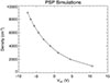 |
Fig. 8. Solar wind density and PSP potential (VSC) using the parameters in Table 5. |
| In the text | |
|
Fig. 9. Variance (Varp) calculated for Encounter 23. For most of each encounter, the variance remains small, less than 1 V. Each encounter has an average maximum (Varp) of approximately 2 V at closest approach, which is ∼10−15% of the measured spacecraft floating potential value. Features in the variance from 50 RS − 55 RS are likely due to the instrument mode transitioning from out-of-encounter to in-encounter. |
| In the text | |
Current usage metrics show cumulative count of Article Views (full-text article views including HTML views, PDF and ePub downloads, according to the available data) and Abstracts Views on Vision4Press platform.
Data correspond to usage on the plateform after 2015. The current usage metrics is available 48-96 hours after online publication and is updated daily on week days.
Initial download of the metrics may take a while.