| Issue |
A&A
Volume 709, May 2026
|
|
|---|---|---|
| Article Number | A228 | |
| Number of page(s) | 14 | |
| Section | Stellar structure and evolution | |
| DOI | https://doi.org/10.1051/0004-6361/202557615 | |
| Published online | 19 May 2026 | |
Testing the 3-equation Kuhfuss convection model using the Sun
1
Max-Planck-Institut für Astrophysik, Karl-Schwarzschild-Straße 1, 85741 Garching, Germany
2
Ludwig-Maximillians-Universität München, Geschwister-Scholl-Platz 1, 80539 Munich, Germany
3
Heidelberger Institut für Theoretische Studien, Schloss-Wolfsbrunnenweg 35, 69118 Heidelberg, Germany
4
Faculty of Comp. Sci. & Appl. Math., Univ. of Applied Sciences, Technikum Wien, Höchstädtplatz 6, A-1200 Wien, Austria
5
Wolfgang-Pauli-Institute c/o Faculty of Mathematics, University of Vienna, Oskar-Morgenstern-Platz 1, A-1090 Wien, Austria
6
Fakultät für Mathematik, Universität Wien, Oskar-Morgenstern-Platz 1, A-1090 Wien, Austria
★ Corresponding author: This email address is being protected from spambots. You need JavaScript enabled to view it.
Received:
9
October
2025
Accepted:
26
March
2026
Abstract
Context. Simplified one-dimensional models are necessary to model convection in the context of stellar evolution. By including the non-local effects of convection, turbulent convection models describe convection in a more physical way than does mixing length theory, which is typically used in one-dimensional stellar evolution models. We recently showed that the 1-equation Kuhfuss turbulent convection model is not sufficient to model the solar convective envelope satisfactorily.
Aims. Using the Sun as a benchmark, we test the physically more complete 3-equation Kuhfuss turbulent convection model.
Methods. We calculated a solar calibrated model with the 3-equation Kuhfuss turbulent convection model using the one-dimensional stellar evolution code GARSTEC. We compared the predicted interior structure of the model with helioseismic measurements of the Sun. Furthermore, we investigated how the free parameters and the closure relations of the 3-equation model affect the results.
Results. We find that with the 3-equation model, the temperature gradient at the inner boundary of the convective envelope is modelled more realistically than with the mixing length theory or the 1-equation model. This also improves the agreement for the sound speed profile between the model and the Sun and reduces the asteroseismic surface effect. However, close to the surface, the 3-equation model results in a layer with an unphysical negative temperature gradient. This layer is connected to the closure relations used in the 3-equation model.
Conclusions. Our results demonstrate the capabilities of turbulent convection models and can serve as a next step towards an improved and more realistic modelling of convection in stellar evolution codes.
Key words: convection / Sun: evolution / Sun: interior
© The Authors 2026
 Open Access article, published by EDP Sciences, under the terms of the Creative Commons Attribution License (https://creativecommons.org/licenses/by/4.0), which permits unrestricted use, distribution, and reproduction in any medium, provided the original work is properly cited.
This article is published in open access under the Subscribe to Open model.
Open access funding provided by Max Planck Society.
1. Introduction
Convection is one of the main energy transport mechanisms in stars, and it is very efficient in mixing chemical elements. Therefore, it is a crucial ingredient in stellar evolution. Convection is an inherently three-dimensional (3D) process, and 3D simulations are important for studying the detailed dynamics in a convective zone (see Käpylä et al. 2023; Lecoanet & Edelmann 2023, and references therein). However, when studying stellar evolution, one-dimensional (1D) stellar evolution codes are needed. This is because modelling convection in 3D is computationally expensive and often not feasible when timescales of stellar evolution are considered (Kupka & Muthsam 2017; Lecoanet & Edelmann 2023). This is due to the several orders of magnitude between the timescale important for convection and that important for stellar evolution. Thus, 1D stellar evolution codes will not become obsolete, and improving their input physics will remain important (Kupka & Muthsam 2017).
The modelling of convection in 1D stellar evolution codes goes back to Ludwig Prandtl, who, in analogy to the mean free path in diffusion processes of gas, introduced the mixing length as a length scale to describe the effects of turbulence (Prandtl 1925). Ludwig Biermann applied this theory to stars (Biermann 1932, 1948). This model, mainly in the formulations developed by Böhm-Vitense (1958) and Cox & Giuli (1968), is known as mixing length theory (MLT) and is widely used in 1D stellar evolution codes (e.g., MESA, CESAM, GARSTEC, Jermyn et al. 2023; Morel & Lebreton 2008; Weiss & Schlattl 2008, respectively; for a review see Joyce & Tayar 2023). It is the most frequently used version of all local convection theories. However, Prandtl (1925) already warned that MLT is merely a crude approximation. This assessment was soon confirmed by disagreements between stellar models and observations. For example, the predicted temperature profile in the envelope of a solar model does not match the solar temperature profile. This leads to disagreements between the theoretical and observed frequencies, the so-called asteroseismic surface effect (Christensen-Dalsgaard et al. 1996). Another example is the convectively mixed core size of intermediate-mass main-sequence stars. MLT predicts these to be too small, resulting in too short main-sequence lifetimes (e.g., Napiwotzki et al. 1991; Chiosi et al. 1992; Zhang 2012; Claret & Torres 2016; Tkachenko et al. 2020).
Disagreements between stellar models and observations, such as convective core sizes being too small, are affected by the local description of convection in MLT. In a local convection model, the decision as to whether a layer is convective is solely based on the state of the fluid at this specific local layer. In the framework of MLT, and when chemical gradients are neglected, this implies that all convective motion comes to a halt at the Schwarzschild boundary. This is the radius where the radiative and adiabatic temperature gradients are equal (∇rad = ∇ad). As a consequence, convective motions immediately cease at the same point at which the buoyancy force, which is the main driving force of convection, disappears. However, due to the inertia of the fluid parcels, it is expected that they penetrate, or overshoot into formally stable layers. The fluid parcels are decelerated until they reach a velocity of zero, thereby transporting energy and elements beyond unstable convective regions. To include this non-local process in a convection model, it needs to be considered that layers through which a fluid parcel travelled at earlier times also affect the characteristics of the fluid parcel. All such non-local processes are generally called convective boundary mixing (CBM; see the review by Anders & Pedersen 2023). There are subcategories based on the effect of CBM on the mixing of elements and the temperature stratification. Overshooting refers to CBM that only extends the chemically mixed region by a certain amount and does not change the temperature stratification. If, in addition to the extended chemical mixing, the temperature stratification in the CBM layer is altered to be close to adiabatic, it is called adiabatic overshooting or convective penetration (Zahn 1991). Convective boundary mixing is observed in 3D simulations (e.g., Hurlburt et al. 1986; Freytag et al. 1996; Käpylä 2019) and is needed to bring models and observations into agreement (e.g., Napiwotzki et al. 1991; Alongi et al. 1991; Chiosi et al. 1992; Demarque et al. 1994). MLT does not account for CBM, and additional mostly parametrised overshooting descriptions were introduced ad hoc to bring models and observations into agreement (e.g., Shaviv & Salpeter 1973; Maeder 1975; Freytag et al. 1996; Anders & Pedersen 2023).
More physically complete turbulent convection models (TCMs) are available, for example Xiong et al. (1997), Kuhfuss (1986, 1987), Canuto & Dubovikov (1998), Deng et al. (2006), Li & Yang (2007). These convection models have the advantage of including the non-local effects already from the start. However, due to the turbulent, and thus, highly non-linear nature of convection, they are more difficult to include in a stellar evolution code. Only a few studies within the framework of stellar evolution codes have been performed so far (e.g., Zhang et al. 2012; Zhang & Li 2012; Zhang 2012; Ahlborn et al. 2022; Braun et al. 2024; Deka et al. 2025).
Kuhfuss developed two models that fall into these more advanced frameworks (Kuhfuss 1986, 1987): the 1- and 3-equation Kuhfuss convection model (1KM and 3KM). Both models are implemented in the GARching STellar Evolution Code (GARSTEC, Weiss & Schlattl 2008) and were improved by Wuchterl & Feuchtinger (1998), Flaskamp (2003), Kupka et al. (2022), and Ahlborn et al. (2022). Both models include non-local effects of convection. The 3KM is physically more complete than the 1KM because it accounts for countergradient fluxes (i.e. positive enthalpy fluxes in locally stably stratified regions; see Sect. 5 for more details on the differences between 1KM and 3KM).
A new convection model first needs to be verified and tested against benchmarks. So far, both Kuhfuss convection models have been successfully tested against the size of convective cores of intermediate-mass main-sequence stars (Ahlborn et al. 2022). Application of the 1KM to Cepheid stars in binary systems confirmed that it can reproduce the observations as well as models applying MLT with ad hoc overshooting (Deka et al. 2025). In a previous paper (Braun et al. 2024), we applied the 1KM in a standard solar model (SSM). This resulted in an adiabatic overshooting layer at the bottom of the convective envelope, leading to a strong disagreement with helioseismic inferences of the solar structure.
Building on these results, we again use the Sun to test the more physically complete 3KM. We find that the 3KM improves the profile of the temperature gradient in the CBM region. The gradual change in the temperature gradient also significantly improves the agreement of the solar model sound speed profile with the sound speed profile of the Sun.
The paper is structured as follows: An overview over 3KM is provided in Sect. 2. In Sect. 3 we briefly discuss the available observables of the Sun and the stellar models we calculated, which are then compared in Sect. 4. We conclude this paper with a discussion (Sect. 5) and a summary and conclusion (Sect. 6). We briefly comment on the effect of an alternative solar composition in Appendix A.
2. The 3-equation Kuhfuss model
To derive the 3-equation Kuhfuss model (3KM), the Reynolds splitting (Reynolds 1895) was applied to the Navier-Stokes and the energy conservation equation. This means that hydrodynamic quantities a were split into a spherically averaged component  and a fluctuating component a′. The 3KM (Kuhfuss 1987) consists of equations for the turbulent kinetic energy (TKE)
  , the second-order entropy fluctuations
  , and the correlation of velocity and entropy fluctuations
  , which is connected to the convective flux Fconv by
 (1)
(1)
with the density ρ and the temperature T. The entropy and velocity fluctuations are denoted by s′ and u′, respectively. u′r is the radial component of the velocity fluctuations. The dynamical equations for ω, Π, and Φ are given as follows:
 (2)
(2)
 (3)
(3)
 (4)
(4)
The bar for mean quantities was omitted to enhance readability. These equations can also describe the time dependence of convection. For this work, we concentrated on studying the main-sequence evolution, where the timescale of stellar evolution is long enough to ensure that convection can reach a steady state. Thus, we neglected the time dependence and set  (a ∈ {ω, Π, Φ}). In the following, we discuss the individual terms constituting the equations of the 3KM in more detail. For a more detailed derivation of the model, we refer to Appendix A by Kupka et al. (2022) and to the original work by Kuhfuss (1987). Further details about the implementation of the 3KM can be found in the works by Flaskamp (2003), Kupka et al. (2022), and Ahlborn et al. (2022).
The driving by buoyancy force, caused by the pressure gradient, is described by the first terms of Eqs. (2) and (3) with the pressure scale height Hp and the adiabatic temperature gradient ∇ad.
The second term in Eq. (2) describes the dissipation of energy, where the dissipation law from Kolmogorov (1941, 1962) was used. The parameter CD is a free parameter. Following Wuchterl (1995), the parameter Λ is calculated by
 (5)
(5)
where r is the radius, α is a free parameter that is typically of order unity, and β is given by the modification derived by Kupka et al. (2022) to include the dissipation by buoyancy waves,
 (6)
(6)
The Brunt-Väisälä frequency  is given by
 (7)
(7)
using the pressure p, the gravitational acceleration g, and the dimensionless mean molecular weight gradient ∇μ. ∇ denotes the dimensionless temperature gradient. The free parameter c4 follows from c4 = c3/(c2cϵ), using model parameters c2 = 1.92 and c3 = 0.3 from Canuto & Dubovikov (1998), and the dissipation rate cϵ = CD in the case of the Kuhfuss model (Ahlborn et al. 2022).
The negative gradient of the specific entropy (∂s/∂r) acts as a driving term for Π and Φ. It is given as
 (8)
(8)
with the specific heat capacity cp. The effects caused by the entropy gradient are described by the second term in Eq. (3) and the first term in Eq. (4). The radiative losses (third term in Eq. (3), and second term in Eq. (4)) are modelled by a typical timescale for radiative cooling of a convective element τrad,
 (9)
(9)
This approximation is based on Vitense (1953) and Böhm-Vitense (1958). The opacity is denoted as κ, the Stefan-Boltzmann constant as σ, and γ is a free parameter.
The third-order moments (TOMs), denoted as ℱa in Eqs. (2) to (4), are modelled by a diffusion approximation,
 (10)
(10)
where a ∈ {ω, Π, Φ}, and αω, αΠ, αΦ are free parameters. These equations introduce the non-local effects into the convection model.
For the equations for Π and Φ (Eqs. (3) and (4)), Kuhfuss (1987) also derived a local closure relation, which is
 (11)
(11)
with a ∈ {Π, Φ}.
The temperature gradient is calculated with
 (12)
(12)
where the radiative diffusivity krad is given as
 (13)
(13)
Similar to MLT, mixing in convective regions is modelled with a diffusion process. The convective velocity vc is obtained from the TKE by assuming full isotropy  , and the diffusion coefficient D is calculated by (Ahlborn et al. 2022)
 (14)
(14)
In summary, the 3KM has seven free parameters: the parameters αω, αΠ, and αΦ are introduced by the modelling of the TOMs, γ affects the timescale of radiative cooling of convective elements, and three more parameters are in the dissipation term of the TKE: CD, α, and c4. The parameters α and c4 also appear in the closure relations for the TOMs. We stress that α does not have the same effect as αMLT in MLT because the convective flux is calculated from an additional differential equation.
Kuhfuss (1987) calibrated the parameters CD, γ, αΠ, and αΦ in the local case against MLT. This led to  ,
,  ,
,  , and
, and  . The overshooting parameter αω = 0.25 was approximated using the 1KM and considering a simple ballistic model. However, for a calibration of the non-local version of 3KM and a better calibration of αω, 3D simulations or comparisons to observations are needed. We refer to Sect. 3.2 for a discussion of the values of the free parameters we used to obtain the models we discuss here.
3. Observations and models
3.1. Observations
The Sun is the ideal benchmark for testing new ingredients in stellar models: the data quality we have is unprecedented because of its proximity. Helioseismology makes it possible to access the interior structure. Below, we give a brief overview of the observables we used for the comparison with solar models. They are the same as discussed by Braun et al. (2024). For more details, we refer to the respective section by Braun et al. (2024) and the review article by Christensen-Dalsgaard (2021) and references therein.
The profile of the solar sound speed is probably one of the most powerful observables for the Sun because it is derived from helioseismic inversions (Basu et al. 2009), which were found to be highly independent of the solar model that is used as reference model (Basu et al. 2000). The temperature gradient of a layer can also be assessed by helioseismology as it affects the sound speed within that layer. Basu & Antia (1997) used models with different depths of the convective envelope and minimised the difference between the profile of the model sound speed and that of the Sun. In this way, the radius at which the temperature gradient changes from close to adiabatic to radiative was found to be Rcz = 0.713 ± 0.001 R⊙ (Basu & Antia 1997). Furthermore, the variation in the adiabatic index caused by the second ionisation zone of helium (He) can be used to measure the He abundance in the convective envelope (Ycz = 0.2485 ± 0.0034, Basu & Antia 2004).
The helioseismic surface effect is the difference between the observed frequencies and the frequencies calculated based on a stellar model. This difference is more pronounced for modes with higher frequencies because they probe layers that lie closer to the surface. This systematic disagreement is caused by insufficient modelling of the convective surface layers in 1D stellar models (structural effect) and by the assumption that the oscillations are adiabatic (modal effect; Houdek et al. 2017). Jørgensen & Weiss (2019) and Zhou et al. (2025) patched an averaged 3D atmosphere to a 1D stellar model to improve the modelling of these surface layers (see also Ball et al. 2016; Belkacem et al. 2019). The surface effect in the patched models is significantly reduced. In particular, the inclusion of turbulent pressure in the stellar model removed the structural effect almost completely. We used their model without turbulent pressure for comparison because our solar model does not include turbulent pressure. We call this patched solar model, with an atmosphere from averaged 3D simulations, but without considering turbulent pressure in the 1D interior, the ‘patched model’ hereafter.
3.2. Solar models
We calculated solar calibrated models with different convection models and compared the interior structure to the observations described above. The stellar evolution code used in this work is GARSTEC1, which was described in detail by Weiss & Schlattl (2008). We obtained solar calibrated models by adjusting the initial helium abundance, Yinit, the initial metal abundance, Zinit, and a free parameter of the convection theory to reproduce the solar radius R⊙, the luminosity L⊙, and the surface metal-to-hydrogen ratio Z⊙/X⊙ at the age of the Sun. As described in Braun et al. (2024), the solar model using MLT (SSM-MLT) was obtained by adjusting the free parameter αMLT to match the solar properties to an accuracy of δA/A⊙ ≲ 2 ⋅ 10−6, with δA = A − A⊙ and A ∈ {R, L, Z/X}. The solar model using the 1-equation model (SSM-1KM) was obtained by varying the equivalent free parameter αΛ until an accuracy of δA/A⊙ ≲ 6 ⋅ 10−5 was reached. All other free parameters of the convection theory were kept constant.
For the solar model with the 3-equation model (SSM-3KM), it is not straightforward to determine the optimal values of the free parameters. In Sect. 2 we mentioned the standard choice for the free parameters, which is based on estimates of Kuhfuss (1987) using the local version of 3KM. For the non-local version, Ahlborn et al. (2022) used αω = αΠ = αΦ = 0.3 for convective cores of intermediate-mass main-sequence stars. They found a good agreement compared to models with classical MLT including overshooting, which were calibrated against observations. To obtain a calibrated solar model, we adjusted αΠ and αΦ, taking the Kuhfuss estimate for the local version of 3KM as guidance, because they have the greatest effect on the effective temperature and the luminosity. After a first approximate adjustment, we kept αΦ = 2.0 constant and continued to vary αΠ to obtain a solar model with an accuracy δA/A⊙ of 10−4 to 10−5. As outlined in Sect. 2, varying the parameter α does not have the same effect as in MLT. In contrast, we found that changing it caused unphysical steps in the temperature gradient because it affects the dissipation by buoyancy waves (Eq. (6)).
For the SSM-3KM described in Sect. 4.1, all free parameters except for αΠ and αΦ were kept at their default value. We acknowledge that this procedure introduces some ambiguity, and the effect of different values for the other free parameters is investigated in Sect. 4.2. We tested the effect of using αΠ = 4.9 and αΦ = 3.3 on convective cores using a 5 M⊙ star. We found that even with these extreme values, the change is minor because a convective core is close to adiabatic, and thus, the temperature gradient is not greatly affected by the choice of parameters (see also Appendix B from Ahlborn et al. 2022). A thorough comparison with 3D hydrodynamical simulations is necessary to calibrate the free parameters of 3KM (Ahlborn et al. 2026).
In all models, the OPAL equation of state (Rogers & Nayfonov 2002) was used. In radiative regions, atomic diffusion was considered for hydrogen, helium, and metals. The models were calibrated to reproduce Z⊙/X⊙ = 0.0225, following the composition of Magg et al. (2022). Our intention was not to study the composition itself, but the effects of a convection model different from MLT. However, we include the solar model using the 3KM and the Asplund et al. (2009) abundances in Appendix A (for a discussion of the effects of composition on the 1KM, see Braun et al. (2024)). The chemical composition used to calculate the opacities is always consistent with the respective solar composition. We used the OP opacities (Badnell et al. 2005), substituted with low-temperature opacities (Ferguson et al. 2005) (Yago Herrera, private communication).
4. Results
This section is divided into three parts. First, we present the results of the fiducial solar calibrated model using the 3KM in Sect. 4.1. This model was obtained by adjusting αΠ while keeping αΦ = 2.0 and the other free parameters of 3KM at their default values. In Sect. 4.2 we study the effect of the free parameters of 3KM. Based on the findings from Sect. 4.1, we test the effect of the local closure relations (Eq. (11)) on the outermost layers in Sect. 4.3.
4.1. Solar model with the 3-equation model
The free parameters we used to obtain the model discussed in this section (the fiducial model) are given in Table 1. In addition, Table 1 states the achieved accuracy of the luminosity, radius, and metal-to-hydrogen ratio and the helium abundance and depth of the convective zone (Ycz and Rcz). The SSM-MLT and SSM-1KM were already discussed in detail by Braun et al. (2024).
4.1.1. The inner boundary
The treatment of convection has a direct effect on the sound speed, which can be measured by helioseismology and can be used to assess the interior structure. Figure 1 shows the relative squared sound speed difference between the helioseismic measurement chelio (Basu et al. 2009) and the model cmodel: δc2/c2 = (chelio2 − cmodel2)/chelio2. The result in the radiative interior is similar to what is obtained with MLT or 1KM, as expected. The most notable difference between the models is the reduction of δc2/c2 below the boundary of the convective region at approximately r = 0.65 R⊙. In this region, 3KM reduces the difference by 37% compared to SSM-MLT and 80% compared to SSM-1KM. Since the sound speed profile is directly affected by the temperature stratification, this is linked to the predicted temperature gradient in the CBM region. At radii ⪆ 0.8 R⊙, the sound speed profile is strongly affected by the accuracy of the calibrated radius, where a small improvement can have a significant effect. Therefore, the effects of the convection theory and the calibration are difficult to separate in this region (see also Appendix B).
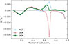 |
Fig. 1. Relative difference of the squared sound speed of the helioseismic measurement chelio and the solar calibrated models cmodel, using MLT (light blue), 1KM (light pink), and 3KM (green). The quantity on the y-axis is defined as δc2/c2 = (chelio2 − cmodel2)/chelio2. The crosses denote the radii of the data points from the helioseismic inversion. |
The upper panel of Fig. 2 shows the temperature gradient at the inner boundary of the solar envelope of SSM-3KM. The temperature gradient of the model (∇) is close to the adiabatic temperature gradient (∇ad) in the layers where ∇ad is smaller than the radiative temperature gradient (∇rad). However, different from SSM-MLT and SSM-1KM, the temperature gradient of SSM-3KM is weakly subadiabatic at radii of 0.716–0.840 R⊙ (−2 ⋅ 10−3 < ∇ − ∇ad < −6.5 ⋅ 10−8, median: −2 ⋅ 10−5) instead of being weakly superadiabatic. Although ∇ < ∇ad, the convective flux Fconv is positive (Fig. 2, lower panel). This defines a Deardorff layer (Deardorff 1966) and is known from 3D simulations (Käpylä et al. 2017; Käpylä 2025) and atmospheric sciences (Deardorff 1966, and references therein). Starting near the Schwarzschild boundary, ∇ smoothly changes from close to ∇ad to ∇rad. In the layer where ∇rad < ∇ < ∇ad, Fconv is negative. Below this layer, Fconv becomes positive again while ∇ ≈ ∇rad and the TKE ω > 0. The value of Fconv in this region is lower by two orders of magnitude than the bulk of the convective zone (maximum 4.0 ⋅ 108 erg/s/cm2 compared to maximum 8.0 ⋅ 1010 erg/s/cm2, median 6.4 ⋅ 1010 erg/s/cm2).
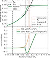 |
Fig. 2. Temperature gradient of the SSM-3KM (green) at the inner boundary of the convective envelope in comparison with the adiabatic (solid black line) and radiative (dashed black line) temperature gradient. The boundary of the convective region as predicted by the model (dotted black line) and as measured by helioseismology (dotted red line) are indicated by vertical lines. The grey shaded regions indicate the 1σ uncertainty of the measurement. The dash-dotted line denotes the radius where ω = 0. The light grey line indicates the temperature profile deduced by Christensen-Dalsgaard et al. (2011). |
Christensen-Dalsgaard et al. (2011) investigated what type of temperature gradient fits the helioseismic data best in the CBM region by parametrising and varying the slope of ∇ without an underlying convection theory. They found that a smooth transition from ∇ad to ∇rad in the CBM region and a subadiabatic stratification in the lower convective zone fits the data best. This optimised temperature profile is included in Fig. 2 (solid grey line). While there are differences in the detailed shape of the temperature gradients derived by Christensen-Dalsgaard et al. (2011) and obtained with 3KM, the overall features of a smoother transition and a subadiabatic stratification already within the Schwarzschild unstable zone agree. This supports the temperature stratification of the SSM-3KM qualitatively.
The vertical lines in Fig. 2 denote the radius at which the TKE becomes zero (dash-dotted line) and the radius at which the change in the slope of ∇ is strongest (dotted black line). These features both leave their imprint on the sound speed profile (see Fig. 3) and are expected to affect the frequencies of the solar oscillations. The transition from a close-to-adiabatic to a radiative temperature gradient (Fig. 2) and its effect on the sound speed profile (Fig. 3) occurs at a radius of 0.7067 R⊙. This lies within 6.3σ of the helioseismic measurement of the depth of the convective envelope (0.713 ± 0.001, Basu & Antia 1997). This is a clear improvement compared to SSM-1KM (29σ, Braun et al. 2024). We note that Basu & Antia (1997) obtained this measurement using convection models that had either no overshooting or overshooting assuming a close-to-adiabatic temperature gradient in the CBM region, which might affect the inferred value for Rcz. A new determination based on SSM-3KM would be necessary. The second feature, which can be seen in Fig. 3, is at a radius of 0.6807 R⊙, which is the same as the radius at which the TKE becomes zero and the mixing of elements stops. This feature is caused by the dependence of the sound speed on molecular weight. However, helioseismology does not detect such a second glitch (Basu & Antia 1997). A more gradual change in molecular weight, resulting from partial mixing, may help to remove this feature.
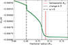 |
Fig. 3. Derivative of the sound speed of the SSM-3KM. The vertical lines denote the boundary of the convective envelope as measured by helioseismology (dotted red) and as predicted by the SSM-3KM (dotted black). The dash-dotted vertical line denotes the radius where ω = 0. The 1σ ranges of the measurement are indicated by the grey shaded region. |
The He abundance of the envelope of SSM-3KM (Ycz = 0.2455; see Table 1) agrees at 0.9σ with the abundance measured by helioseismology (Ycz = 0.2485 ± 0.0034, Basu & Antia 2004). In short, the 3KM with standard parameters agrees much better with the sound speed profile of the Sun than the standard MLT model, and it agrees very well in Ycz with the seismic value. 3KM improves Rcz compared to 1KM, and it deviates by 6.3σ from the value determined by Basu & Antia (1997), which itself may need to be redetermined by using solar models with a non-local convection theory. Based on the sound speed profile of the 3KM, two glitches, caused by the change in molecular weight and the temperature gradient, would be expected. This does not agree with helioseismology.
4.1.2. The outer boundary
The profiles of the temperature gradient at the upper boundary of the convective zone, that is, immediately below the surface, predicted by MLT and 1KM, are very similar. They predict a weakly superadiabatic temperature gradient in the bulk of the convective region, which becomes strongly superadiabatic close to the surface (MLT: ∇ − ∇ad = 0.55 at r/R⊙ = 0.99992; 1KM: ∇ − ∇ad = 0.46, at r/R⊙ = 0.99991). In the SSM-3KM this superadiabatic layer (SAL) has a stronger superadiabaticity of ∇ − ∇ad = 1.25 (at r/R⊙ = 0.99989; see Fig. 4). Towards smaller radii, the temperature gradient becomes subadiabatic and even negative (0.9981–0.9997 R⊙, minimum ∇ = −3.7 ⋅ 10−3), before it becomes weakly superadiabatic (0.8394–0.9981 R⊙, median: ∇ − ∇ad = 2.2 ⋅ 10−4). We used hydrodynamical simulations of the solar atmosphere from the literature to compare the temperature stratification in the outer layers. Figure 5 shows the temperature gradient against temperature. The temperature inversion in SSM-3KM is shown in detail in the inset in this figure, which zooms in on the relevant region. This can be compared to the patched model, which uses the averaged 3D simulation from the STAGGER grid (Magic et al. 2013; Jørgensen & Weiss 2019; Zhou et al. 2025, black, dashed line in Fig. 5). These 3D simulations clearly do not include a layer with a negative temperature gradient, nor do the 2D simulations presented in Schlattl et al. (1997, their Fig. 2).
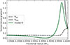 |
Fig. 4. Temperature stratification of the outer 0.0015 R⊙ of the SSM-3KM. |
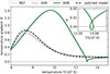 |
Fig. 5. Temperature gradient against the temperature of SSM-MLT (light blue), SSM-1KM (light pink), and SSM-3KM (green). The thick dashed line shows the temperature gradient of the patched model (Jørgensen & Weiss 2019). The temperature range we show corresponds to the outermost 0.0017 R⊙. The inset shows a zoom-in into the region with a negative temperature gradient. |
The outer layers also affect the helioseismic surface effect. Using GYRE (Townsend & Teitler 2013), we calculated the frequencies of the solar models with the different convection theories (see Appendix C for more details). We found an improvement in the surface effect (Fig. 6). The maximum absolute difference between the observed and modelled frequencies decreases from 16.0 μHz to 6.3 μHz when the 3KM is applied in comparison to MLT (1KM: 18.3 μHz). Demarque et al. (1997, 1999) found that a stronger superadiabaticity in the SAL reduces the surface effect, which agrees with the properties of the SSM-3KM (Fig. 5). However, the patched model (Jørgensen & Weiss 2019; Zhou et al. 2025) improves the surface effect without having a stronger superadiabaticity in the SAL compared to SSM-MLT and SSM-1KM. This suggests that the surface effect does not depend on the superadiabaticity of the SAL alone.
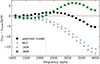 |
Fig. 6. Helioseismic surface effect, i.e. the mismatch between the observed frequencies and those calculated from SSM-MLT (light blue), SSM-1KM (light pink), SSM-3KM (green), and the solar model using an averaged 3D atmosphere as the outer boundary condition (“patched model”, black, Jørgensen & Weiss 2019). |
Figure 7 shows the pressure against temperature in the uppermost layers. The patched model has a higher temperature for a given pressure for log P/Ba ⪅ 6.5 than SSM-1KM and SSM-MLT. The higher temperature at a given pressure in this range seems to be a common characteristic of the patched model (Jørgensen & Weiss 2019; Zhou et al. 2025), the 2D simulation (Schlattl et al. 1997), and the SSM-3KM, which all improve the surface effect, but have otherwise different relations of pressure and temperature and different profiles of ∇ in the SAL.
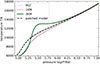 |
Fig. 7. Pressure against temperature in the uppermost regions. The light pink line shows the profile for SSM-1KM, which largely overlaps the light blue line showing the SSM-MLT. The dashed black line shows the profile of the solar model using an averaged 3D atmosphere as the outer boundary condition (“patched model”, Jørgensen & Weiss 2019). SSM-3KM is represented by the green line. The segment corresponds to the outermost 0.0026 R⊙. |
Finally, the structure of the SAL also affects the effective temperatures of the models. The solar models have the same effective temperature by construction. The effect on the effective temperatures, however, becomes relevant in the later evolutionary stages. Starting from the solar calibrated models, we continued the evolution up the RGB. When the 1KM is used instead of MLT, only minor differences arise in the effective temperatures along the RGB evolution. The model using 3KM, in contrast, evolves at lower effective temperatures than for 1KM or MLT. A more detailed study is needed to clarify whether the shift in effective temperature as seen when using 3KM is favourable (see also Fig. 12, and Sect. 5.2).
In summary, the 3KM includes non-local effects without any ad hoc description, different from convection models assuming instant mixing over a fraction of the pressure scale height. It improves the temperature stratification at the inner boundary of the convective region. However, especially at the outer boundary, features arise that are unrealistic (particularly the local temperature inversion around T ∼ 13 ⋅ 103 K). Next, we therefore studied whether choosing different model parameters can remove these discrepancies and improve the solar model. Furthermore, in Sect. 4.3, we test the effect of the local closure relations of the Π and Φ equation.
4.2. Effects of varying free parameters
The SSM-3KM discussed in Sect. 4.1 (fiducial model) used a specific set of the free parameters of the 3KM. However, other parameter combinations can also result in solar calibrated models. To test the effect of the different parameters on the interior structure, we changed the value of one parameter at a time and calibrated the model by varying αΠ, as before. Table 1 gives an overview of the parameters we used, the resulting values for αΠ, δR/R⊙, δL/L⊙, and δ(Z/X)/(Z⊙/X⊙), and for the He content Ycz and the depth Rcz of the convective envelope.
All sets of parameters resulted in solar models that fit the helioseismic measurement of the helium abundance in the convective envelope by < 1.4σ (Ycz = 0.2485 ± 0.0034, Basu & Antia 2004). For models with a deeper convective envelope, the agreement is better.
The left panels in Fig. 8 show the sound speed profiles of the models with different combinations of free parameters. Even when the outer layers are ignored, which are strongly affected by the exact radius of the model (see Appendix B), differences can be seen at the inner boundary of the convective region. Investigation of the profile of the temperature gradient shows that the slope of the temperature gradient in the CBM region is correlated with the prominent feature around 0.65 R⊙: the steeper the change in ∇ (see right panels of Fig. 8), the larger the difference between model and observations in the sound speed profile in this region. This supports the finding of Christensen-Dalsgaard et al. (2011) that a smooth change from ∇ ≈ ∇ad to ∇rad agrees best with helioseismic data.
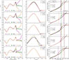 |
Fig. 8. Solar models obtained with the 3KM and different sets of free parameters (see Table 1). From left to right, the panels show the difference of the sound speed profile between models and observations, the temperature stratification of the outer layers, and the temperature stratification at the inner boundary of the convective envelope. The vertical lines in the right panels denote the radius at which the change of the slope in the profile of the temperature gradient is strongest. The dotted red line denotes the helioseimisc measurement, with the 1σ ranges indicated by the grey shaded regions. |
The base of the convective envelope, marked with vertical lines in the right panels of Fig. 8, shows the opposite. When the change of ∇ to ∇rad is more gradual, Rcz is at smaller radii and therefore disagrees stronger with the helioseismic measurement by Basu & Antia (1997) of 0.713 ± 0.001 R⊙.
The models that show a larger improvement in the sound speed profile do not necessarily give a better result at the surface layers (middle panels in Fig. 8). For example, the model with αΦ = 1.0 results in a very smooth change from ∇ ≈ ∇ad to ∇rad, but the temperature gradient becomes more negative at T ≈ 13 ⋅ 103 K compared to the fiducial parameter combination, or most of the other models. Furthermore, in all cases, the subadiabatic region between the SAL and the second superadiabatic region persists.
The parameters can be classified based on the region they affect most. The parameters αω and c4 mainly affect the inner boundary of the convective region. This is because αω controls the non-local part of the TKE equation and c4 controls the dissipation by buoyancy waves, which only affects the CBM region. The parameter γ has only a minor effect on the inner boundary of the convective region. Its main effect is at the outer boundary, where radiative losses become significant. The other parameters, αΦ and CD, affect both boundaries of the convective region.
In summary, we conclude that the unrealistic strongly subadiabatic temperature gradient below the superadiabatic peak is likely not an artefact of a poor parameter choice, but a sign that the convection model itself needs further improvement. In addition, comparisons to 3D simulations are needed to study and calibrate the free parameters of the 3KM because the effect of the individual parameters on the structure is too intertwined to calibrate them based on observational data.
4.3. Alternative closure relations for Π and Φ
To test the origin of the unrealistic layer below the SAL, we used the local closure relations for the Π and Φ equations (Eq. (11)) for r/R⊙ ⪆ 0.979 instead of the non-local ones, which we continued to use for r/R⊙ ⪅ 0.979 (Eq. (10)). We distinguished three cases. In case A, the TOMs of the equations for Φ and for Π were both modelled with the local closure relation. In case B (case C), we used the local closure relation for Φ (Π) and the non-local closure relation for Π (Φ; see Table 2 for an overview of the different cases). For all cases, αΠ needed to be adjusted to obtain a solar model with the correct radius and luminosity. All other free parameters had the same values as in the fiducial model. Table 1 shows the values for αΠ and the achieved accuracy.
Treatment of the TOMs of the Π and Φ equation of the different cases.
Switching to local closure relations in the outer layers of the model clearly introduces inconsistency in the solar model. At the switch point, the shift from the fully non-local 3KM to a version with at least one local closure relation causes a jump in the temperature gradient of varying degree (see Fig. 9), the largest one in case C. For case A, ∇ jumps from sub- to superadiabatic at the switch point. For case B, the jump is smallest. However, these calculations are only meant as a test to understand better which term causes the unrealistic behaviour of the outermost layers. The effect on the inner boundary of the convective envelope when switching to the local closure relations in the outermost layers is only minor. For all cases, the temperature gradient no longer becomes negative. Since the different treatment of the closure relations is only applied to the outermost layers, the subadiabatic region between the SAL and a second superadiabatic region persists. The details of the profiles of the temperature gradients are different between the cases.
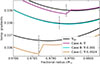 |
Fig. 9. Radius at which the models switch to the local closure relations for the outer regions. Case A is shown in purple. For better visibility, case B (turquoise) and case C (orange) are shifted by –0.001 and –0.0024, respectively (see Table 2). The black lines show ∇ad of the different models, shifted by the same amount as the model ∇. The dotted vertical lines mark the last grid point at which the fully non-local 3KM was applied. |
The profile of the temperature gradient of case A shows the most direct similarity to SSM-MLT and SSM-1KM (see Fig. 10). Except for a larger temperature gradient (∇ = 1.27) and a slight shift of the peak of the SAL to 7.4 ⋅ 103 K, it agrees with the profiles of SSM-MLT (∇ = 0.89 at 7.1 ⋅ 103 K) and SSM-1KM (∇ = 0.77 at 7.6 ⋅ 103 K). A weakly superadiabatic region (mean ∇ − ∇ad ∼ 1.8 ⋅ 10−3) follows directly below the SAL. In the regions in which the fully non-local 3KM was applied, the behaviour of the temperature gradient is as in the other models. The similarity of MLT and case A is also visible in the surface effect (Fig. 11). The evolution of case A in the HRD is the same as for MLT and 1KM until it reaches the lower RGB (see Fig. 12). Thereafter, the effective temperature continuously increases compared to the models using MLT or 1KM.
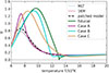 |
Fig. 10. Temperature gradient against temperature of the uppermost layers. The temperature range shown corresponds to the uppermost 0.0034 R⊙. The thin light blue and light pink lines show the profiles for SSM-MLT and SSM-1KM, respectively. The dashed black line shows the profile of a solar model using an averaged 3D atmosphere as outer boundary condition (“patched model”, Jørgensen & Weiss 2019). The green, purple, turquoise, and orange lines show the profiles for the fully non-local 3KM, and for case A, case B, and case C, respectively (see Table 2). |
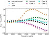 |
Fig. 11. Surface effect of the solar models with different closure relations for the 3KM in the outer regions (fully non-local: green; case A: purple; case B: turquoise; case C: orange; see Table 2). The result for SSM-MLT (light blue triangles), SSM-1KM (light pink dots), and the patched model (black, Jørgensen & Weiss 2019) are shown for comparison. |
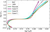 |
Fig. 12. Hertzsprung-Russel diagram showing the evolution of the solar models. The models using MLT and the 1KM are shown in thin light blue and light pink lines for comparison. The different treatment of the outer layers for the models with 3KM results in higher (Case A: purple) and lower (fully non-local: green; Case B: turquoise; Case C: orange) effective temperatures on the RGB compared to MLT and 1KM. |
Cases B and C result in a subadiabatic region below the SAL (Fig. 10). The SAL is broader for case C (ΔT = 7.9 ⋅ 103 K). The peak of this region is at 8.6 ⋅ 103 K, which is between the peak of the SSM-MLT and the fiducial model. The change from a super- to a subadiabatic temperature gradient is very gradual. This results in a surface effect that is even more positive (νobs > νmodel; Fig. 11) than for the fiducial model. Case B has a narrower SAL (ΔT = 5.8 ⋅ 103 K), and the change to the subadiabatic temperature gradient is less gradual. The peak of the SAL (∇ = 1.3 at 9.5 ⋅ 103 K) is closer to what was obtained with the fully non-local 3KM. This profile results in frequencies that decrease the difference between observed and theoretical frequencies compared to the fully non-local case. For this model, the surface effect is also closest to what was obtained with the patched solar model, although the structure of the SAL is different. This again shows that direct conclusions cannot clearly be drawn about the surface effect from the temperature stratification in the outer layers alone. In the HRD, cases C and B are at lower effective temperatures along the RGB. Case C starts the RGB at cooler temperatures, but follows the fully non-local 3KM closely afterwards. The effective temperature on the RGB for case B is between the one obtained when using MLT or 1KM and the fully non-local 3KM.
The shift in effective temperature between the different cases is the result of different convective fluxes in the models. The higher convective flux of case A causes the radius to be smaller, which means that the temperature is higher at a given luminosity. The lower effective temperatures of the fiducial model, case C, and case B are due to their lower convective flux. The thin layer at which the different closure relations are used affects the bulk of the convective zone enough to result in the shift in effective temperature seen on the RGB, although the temperature stratification at the inner boundary is not affected (see Sect. 5.2 for a discussion about observational uncertainties).
Since none of these cases show a negative temperature gradient, it is clear that the unrealistic modelling of the outer layers is caused by the closure relations of the Φ and/or Π equation. The coupling of the equations makes it difficult to see exactly which of the two is the main contributor to this behaviour, but improving these terms can be an ansatz to further develop the 3-equation Kuhfuss model (Kupka 2026).
5. Discussion
In Sect. 5.1 we discuss the main difference between the 1KM and 3KM and the effect of it, that is, the application of the downgradient approximation for the convective flux in 1KM that was replaced in 3KM by solving Eqs. (3) and (4). The results are compared to the literature in Sect. 5.2.
5.1. Differences in the convection models
In addition to the inclusion of non-local effects, which are also included in 1KM, the most significant difference between MLT and 1KM compared to the 3KM is the modelling of the convective flux, which affects and explains the profile of ∇ in the SSM-3KM. MLT and 1KM both assume that the convective flux is proportional to the entropy gradient, that is,
 (15)
(15)
which ties the sign of Fconv to the superadiabaticity of the layer. For 3KM, this downgradient approximation is not applied (see Eq. (3)) and the convective flux has contributions from the superadiabatic gradient and from the entropy fluctuations. Together with the inclusion of the non-local effects of the entropy fluctuations (Deardorff 1966), this makes it possible to have a Deardorff layer: a layer with ∇ − ∇ad < 0 and Fconv > 0 (Deardorff 1966; Chan & Gigas 1992; Tremblay et al. 2015; Käpylä et al. 2017; Andrassy et al. 2024; Käpylä 2025). It also weakens the coupling between chemical mixing and changes in the thermal structure. Thus, the mixed region extends into layers with a close-to-radiative temperature gradient, another feature that is not obtained with the 1KM and similar convection models.
When we compare Eq. (3), the equation describing the convective flux, with Eq. (14) from the derivation by Brandenburg (2016), it becomes clear that Brandenburg arrived at a very similar model as 3KM from a slightly different ansatz. With this ansatz, Brandenburg (2016) found convection zones with extended Deardorff layers, with long narrow plumes reaching from close to the surface far into regions with a subadiabatic temperature gradient. These plumes are highly non-local and are driven by the surface cooling. This effect is called entropy rain. In 3D simulations, Deardorff layers often only extend over a limited range of the convective region (Käpylä et al. 2017), similar to what 3KM predicts for the Sun. However, Käpylä (2025) tested whether an extended entropy rain, as discussed by Brandenburg (2016), can be realised in 3D simulations. Instead of assuming uniform cooling, Käpylä (2025) applied non-uniform cooling patches to the upper boundary of the 3D simulation, taking the non-uniform surface temperature of the Sun as inspiration. He found that with this set-up, the bulk of the convective zone is subadiabatic, with fast, narrow downflows. From observational data, Bekki (2024) found evidence that the bulk of the solar convective envelope is less superadiabatic than usually assumed, or even subadiabatic. These studies indicate that subadiabatic convection may be present in the solar envelope. This would imply that MLT does not accurately represent the temperature stratification due to its underlying assumptions. The 3KM constitutes an important step towards a more realistic representation of such subadiabatic convection in 1D stellar evolution codes.
5.2. Comparison to the literature
The determination of Rcz involves comparing and minimising the difference of the sound speed between the Sun and a reference model (Basu & Antia 1997). The reference models used by Basu & Antia (1997) to determine Rcz either did not include overshooting or did include it in the sense of adiabatic overshooting, that is, the temperature gradient in the CBM region is assumed to be close to adiabatic, with a sharp transition to ∇rad at the boundary. With these reference models, they found that the change in the temperature gradient occurred at a radius of 0.713 ± 0.001 R⊙ (Basu & Antia 1997). It is unclear whether this result is directly applicable to the SSM-3KM because the change in ∇ is much smoother than in the reference models used to derive this value. The measurement of Rcz needs to be repeated with models with a smooth transition in the temperature gradient, such as the SSM-3KM, to assess which effect the profile of ∇ of the stellar model has on the measurement of Rcz.
The measurement of Rcz is further complicated by composition gradients at the base of the convective zone (Basu & Antia 1994). Basu & Antia (1997) used different models to determine the composition profile that fits the signatures from helioseismology best. They found that only models with a smooth composition profile were consistent with the observations. The additional feature in the derivative of the sound speed of SSM-3KM indicates that 3KM predicts a composition profile that is too sharp. A more gradual damping of the TKE or additional effects such as shear flows due to rotation (Richard et al. 1996; Basu 1997) might help to smooth out the composition profile in the transition region from convective to radiative.
Christensen-Dalsgaard et al. (2011) parametrised the temperature stratification below the convective region to be able to vary how smoothly the temperature gradient changed from close to ∇ad to ∇rad. The temperature stratification that Christensen-Dalsgaard et al. (2011) found to agree best with the helioseismic data qualitatively agrees with the profile predicted by 3KM. A smooth change from ∇ad to ∇rad was also found in the 3D hydrodynamical simulations from Käpylä et al. (2017). Xiong (1989) developed a TCM similar to the 3KM, which was extended to include anisotropic effects by Deng et al. (2006). Xiong & Deng (2001) used this convection model to calculate an envelope model for the Sun, which was used as reference model for helioseismic inversions by Zhang et al. (2012) (for an overview of this convection theory and the tests performed, see Xiong (2021), and references therein). They found that the transition of ∇ from close to adiabatic to radiative is smooth and that ∇ is already subadiabatic within the formally unstable layer (Xiong & Deng 2001). They also found that this improved the sound speed profile (Zhang et al. 2012). Similar results were found by Zhang & Li (2012). They used the TCM developed by Li & Yang (2007) to calculate an evolutionary model of the Sun. Again, using a TCM improved the sound speed profile and led to a smoother transition of the temperature gradient in the CBM region. The 3KM agrees qualitatively with these other convection models regarding the smoother transition in the temperature gradient at the lower boundary and the resulting improvement in the sound speed profile. However, these other works did not predict a subadiabatic region close to the SAL, as is the case when using 3KM.
Rempel (2004) approached the problem of the CBM at the base of the solar convection zone with a semi-analytical convection model, considering individual plumes reaching from the top of the convective zone to the bottom. With this model, they also found an extended Deardorff layer and a smoother transition from a close-to-adiabatic to a radiative temperature gradient at the lower boundary of the convective zone. The smoothness of the transition of the temperature gradient depended mainly on the free parameter that controls the ratio of the dimensionless total energy flux and the filling factor of the downward plumes at the base of the convective envelope. The authors argued that non-local extensions of MLT result in adiabatic overshoot not because of crude approximations, but because of the assumption of a large filling factor. The difference between the models by Xiong & Deng (2001) and by Rempel (2004) is concluded in the latter to stem from the dominant breaking process in the CBM region, which is buoyancy breaking in Rempel (2004) as opposed to turbulent dissipation in Xiong & Deng (2001). In the 3KM, the dominant breaking process in the CBM region is also turbulent dissipation. In contrast to the model by Xiong & Deng (2001), however, 3KM takes dissipation due to buoyancy waves into account (Kupka et al. 2022). In conclusion, the different convection models obtain the same result of a Deardorff layer and a smooth transition to the radiative temperature gradient despite considering different physical processes.
The effective temperature on the RGB is cooler when 3KM is used compared to 1KM or MLT. This shift does not immediately rule out the 3KM because stellar models with a solar calibrated αMLT were found to disagree with some observations (Bonaca et al. 2012; Creevey et al. 2015; Joyce & Chaboyer 2018a,b; Viani et al. 2018). In particular, Tayar et al. (2017) found that stellar models with a solar calibrated αMLT differ from the effective temperatures of red giants, although this study was challenged by Salaris et al. (2018) and Choi et al. (2018). Detailed studies are needed before we can conclude whether the change in effective temperature on the RGB for solar models using 3KM is desirable or not.
The closure relations for the TOMs of the Π and Φ equation have a strong effect on the SAL and on the subadiabatic layer below it. Therefore, they also affect the effective temperature on the RGB. The closure relations must be improved to remove the artefact of the temperature inversion in these layers when using the 3KM with the non-local closure relations for all equations. Work developing new closure relations for 3KM is currently underway (Kupka 2026).
6. Conclusion and summary
We calculated a solar model using the non-local 3-equation Kuhfuss turbulent convection theory (3KM, Kuhfuss 1987; Kupka et al. 2022; Ahlborn et al. 2022). In addition to the non-locality, the main difference between 3KM and classical MLT is the inclusion of the second-order entropy fluctuations contributing to the convective flux.
The 3KM improves the modelling of the convective boundary mixing region. It reproduces the temperature stratification at the inner boundary of the convective zone in qualitative agreement to the optimal stratification inferred by Christensen-Dalsgaard et al. (2011) from helioseismic measurements. 3KM also predicts a Deardorff layer, which is especially interesting as first observations suggest that the solar convective envelope in some regions is less superadiabatic than previously assumed, or it might even be subadiabatic (Bekki 2024). The inclusion of the second-order entropy fluctuations is crucial for obtaining a Deardorff layer and a smooth transition of the temperature gradient in the convective boundary mixing region. Furthermore, the agreement of the sound speed profile between helioseismic measurements and the stellar model is significantly improved.
While the temperature stratification of the lower boundary of the convective envelope is significantly improved when using 3KM, problematic features arise at the upper boundary. Immediately below the superadiabatic layer, the temperature gradient becomes strongly subadiabatic and even negative, before it becomes superadiabatic again. This feature is not observed in 3D simulations and is not described in the literature covering other 1D descriptions of non-local convection. We investigated whether these features are connected to a specific choice of parameters, but we are unable to confirm a clear correlation between one specific free parameter and the features described above. Instead, we showed that different combinations produce solar models with similar features, but different details. Due to the interplay between the free parameters, it is not possible to calibrate all of them with the limited observations we have. To further constrain their values, a comparison with 3D simulations is needed.
With the goal of better understanding which term causes the unrealistic behaviour just below the superadiabatic layer, we calculated models using the local closure relations (Eq. (11)) for the Π and Φ equation in the outer ≈0.021 R⊙. The inner boundary of the convective region is not affected significantly. In the outer layers, this results in a temperature stratification that agrees better with MLT and 3D simulations because the temperature gradient no longer becomes negative. However, there is still a subadiabatic region between the superadiabatic peak region and a second superadiabatic region, which is likely unphysical and not observed in the 3D simulations. Since these equations are coupled and all versions result in a non-negative temperature gradient, it is not obvious which of the two terms is the main contributor. It becomes clear that improving the closure relation of the Π and Φ equation is a promising ansatz to further develop this model (see Kupka 2026).
Thus, the 3KM can serve as a starting point to develop a new convection theory. While still showing some limitations, the 3KM is clearly a step forward to improve the modelling of convection in 1D stellar evolution codes.
Acknowledgments
We thank Sarbani Basu for productive discussions of the helioseismic observables. We thank Yago Herrera for providing the opacity tables with the updated solar composition. We thank Andreas Jørgensen for providing the data of the patched solar model. FK is grateful for the hospitality provided by the Wolfgang Pauli Institute, Vienna, and acknowledges support by the Faculty of Mathematics at the University of Vienna through offering him a Senior Research Fellow status – the Austrian Science Fund (FWF) has supported this research through grants P 33140-N, P 35485-N, and PAT1338425. FA acknowledges funding from the European Research Council under the European Community’s Horizon 2020 Framework/ERC grant agreement no 101000296 (DipolarSounds) and thanks the Klaus Tschira foundation for their support.
References
- Ahlborn, F., Kupka, F., Weiss, A., & Flaskamp, M. 2022, A&A, 667, A97 [NASA ADS] [CrossRef] [EDP Sciences] [Google Scholar]
- Ahlborn, F., Higl, J., Andrassy, R., et al. 2026, A&A, 705, A191 [NASA ADS] [CrossRef] [EDP Sciences] [Google Scholar]
- Alongi, M., Bertelli, G., Bressan, A., & Chiosi, C. 1991, A&A, 244, 95 [NASA ADS] [Google Scholar]
- Anders, E. H., & Pedersen, M. G. 2023, Galaxies, 11, 56 [NASA ADS] [CrossRef] [Google Scholar]
- Andrassy, R., Leidi, G., Higl, J., et al. 2024, A&A, 683, A97 [NASA ADS] [CrossRef] [EDP Sciences] [Google Scholar]
- Asplund, M., Grevesse, N., Sauval, A. J., & Scott, P. 2009, ARA&A, 47, 481 [NASA ADS] [CrossRef] [Google Scholar]
- Asplund, M., Amarsi, A. M., & Grevesse, N. 2021, A&A, 653, A141 [NASA ADS] [CrossRef] [EDP Sciences] [Google Scholar]
- Badnell, N. R., Bautista, M. A., Butler, K., et al. 2005, MNRAS, 360, 458 [Google Scholar]
- Ball, W. H., Beeck, B., Cameron, R. H., & Gizon, L. 2016, A&A, 592, A159 [NASA ADS] [CrossRef] [EDP Sciences] [Google Scholar]
- Basu, S. 1997, MNRAS, 288, 572 [NASA ADS] [Google Scholar]
- Basu, S., & Antia, H. M. 1994, MNRAS, 269, 1137 [NASA ADS] [Google Scholar]
- Basu, S., & Antia, H. M. 1997, MNRAS, 287, 189 [NASA ADS] [CrossRef] [Google Scholar]
- Basu, S., & Antia, H. M. 2004, ApJ, 606, L85 [CrossRef] [Google Scholar]
- Basu, S., Pinsonneault, M. H., & Bahcall, J. N. 2000, ApJ, 529, 1084 [NASA ADS] [CrossRef] [Google Scholar]
- Basu, S., Chaplin, W. J., Elsworth, Y., New, R., & Serenelli, A. M. 2009, ApJ, 699, 1403 [NASA ADS] [CrossRef] [Google Scholar]
- Bekki, Y. 2024, A&A, 682, A39 [NASA ADS] [CrossRef] [EDP Sciences] [Google Scholar]
- Belkacem, K., Kupka, F., Samadi, R., & Grimm-Strele, H. 2019, A&A, 625, A20 [EDP Sciences] [Google Scholar]
- Biermann, L. 1932, Veroeffentlichungen der Universitaets-Sternwarte zu Goettingen, 0002, 220.1 [Google Scholar]
- Biermann, L. 1948, Z. Astrophys., 25, 135 [Google Scholar]
- Böhm-Vitense, E. 1958, Z. Astrophys., 46, 108 [Google Scholar]
- Bonaca, A., Tanner, J. D., Basu, S., et al. 2012, ApJ, 755, L12 [NASA ADS] [CrossRef] [Google Scholar]
- Brandenburg, A. 2016, ApJ, 832, 6 [Google Scholar]
- Braun, T. A. M., Ahlborn, F., & Weiss, A. 2024, A&A, 689, A292 [NASA ADS] [CrossRef] [EDP Sciences] [Google Scholar]
- Buldgen, G., Salmon, S. J. A. J., Noels, A., et al. 2019, A&A, 621, A33 [NASA ADS] [CrossRef] [EDP Sciences] [Google Scholar]
- Buldgen, G., Eggenberger, P., Noels, A., et al. 2023, A&A, 669, L9 [NASA ADS] [CrossRef] [EDP Sciences] [Google Scholar]
- Buldgen, G., Noels, A., Baturin, V. A., et al. 2025, A&A, 700, A50 [NASA ADS] [CrossRef] [EDP Sciences] [Google Scholar]
- Canuto, V. M., & Dubovikov, M. 1998, ApJ, 493, 834 [NASA ADS] [CrossRef] [Google Scholar]
- Chan, K. L., & Gigas, D. 1992, ApJ, 389, L87 [NASA ADS] [CrossRef] [Google Scholar]
- Chiosi, C., Wood, P., Bertelli, G., & Bressan, A. 1992, ApJ, 387, 320 [NASA ADS] [CrossRef] [Google Scholar]
- Choi, J., Dotter, A., Conroy, C., & Ting, Y.-S. 2018, ApJ, 860, 131 [NASA ADS] [CrossRef] [Google Scholar]
- Christensen-Dalsgaard, J. 2008, Ap&SS, 316, 113 [Google Scholar]
- Christensen-Dalsgaard, J. 2021, Liv. Rev. Sol. Phys., 18, 2 [NASA ADS] [CrossRef] [Google Scholar]
- Christensen-Dalsgaard, J., Dappen, W., Ajukov, S. V., et al. 1996, Science, 272, 1286 [Google Scholar]
- Christensen-Dalsgaard, J., Monteiro, M. J. P. F. G., Rempel, M., & Thompson, M. J. 2011, MNRAS, 414, 1158 [CrossRef] [Google Scholar]
- Claret, A., & Torres, G. 2016, A&A, 592, A15 [NASA ADS] [CrossRef] [EDP Sciences] [Google Scholar]
- Cox, J. P., & Giuli, R. T. 1968, Principles of Stellar Structure (Gordon and Breach) [Google Scholar]
- Creevey, O. L., Thévenin, F., Berio, P., et al. 2015, A&A, 575, A26 [NASA ADS] [CrossRef] [EDP Sciences] [Google Scholar]
- Deardorff, J. W. 1966, J. Atmos. Sci., 23, 503 [NASA ADS] [CrossRef] [Google Scholar]
- Deka, M., Ahlborn, F., Braun, T. A. M., & Weiss, A. 2025, A&A, 699, A351 [NASA ADS] [CrossRef] [EDP Sciences] [Google Scholar]
- Demarque, P., Sarajedini, A., & Guo, X. J. 1994, ApJ, 426, 165 [NASA ADS] [CrossRef] [Google Scholar]
- Demarque, P., Guenther, D. B., & Kim, Y.-C. 1997, ApJ, 474, 790 [Google Scholar]
- Demarque, P., Guenther, D. B., & Kim, Y.-C. 1999, ApJ, 517, 510 [Google Scholar]
- Deng, L., Xiong, D. R., & Chan, K. L. 2006, ApJ, 643, 426 [NASA ADS] [CrossRef] [Google Scholar]
- Ferguson, J. W., Alexander, D. R., Allard, F., et al. 2005, ApJ, 623, 585 [Google Scholar]
- Flaskamp, M. 2003, Ph.D. Thesis, Munich University of Technology, Germany [Google Scholar]
- Freytag, B., Ludwig, H. G., & Steffen, M. 1996, A&A, 313, 497 [NASA ADS] [Google Scholar]
- Grevesse, N., & Sauval, A. J. 1998, Space Sci. Rev., 85, 161 [Google Scholar]
- Houdek, G., Trampedach, R., Aarslev, M. J., & Christensen-Dalsgaard, J. 2017, MNRAS, 464, L124 [Google Scholar]
- Hurlburt, N. E., Toomre, J., & Massaguer, J. M. 1986, ApJ, 311, 563 [NASA ADS] [CrossRef] [Google Scholar]
- Jermyn, A. S., Bauer, E. B., Schwab, J., et al. 2023, ApJS, 265, 15 [NASA ADS] [CrossRef] [Google Scholar]
- Jørgensen, A. C. S., & Weiss, A. 2019, MNRAS, 488, 3463 [Google Scholar]
- Joyce, M., & Chaboyer, B. 2018a, ApJ, 864, 99 [NASA ADS] [CrossRef] [Google Scholar]
- Joyce, M., & Chaboyer, B. 2018b, ApJ, 856, 10 [Google Scholar]
- Joyce, M., & Tayar, J. 2023, Galaxies, 11, 75 [NASA ADS] [CrossRef] [Google Scholar]
- Käpylä, P. J. 2019, A&A, 631, A122 [NASA ADS] [CrossRef] [EDP Sciences] [Google Scholar]
- Käpylä, P. J. 2025, A&A, 698, L13 [NASA ADS] [CrossRef] [EDP Sciences] [Google Scholar]
- Käpylä, P. J., Rheinhardt, M., Brandenburg, A., et al. 2017, ApJ, 845, L23 [CrossRef] [Google Scholar]
- Käpylä, P. J., Browning, M. K., Brun, A. S., Guerrero, G., & Warnecke, J. 2023, Space Sci. Rev., 219, 58 [CrossRef] [Google Scholar]
- Kolmogorov, A. 1941, Dokl. Akad. Nauk SSSR, 30, 301 [NASA ADS] [Google Scholar]
- Kolmogorov, A. N. 1962, J. Fluid Mech., 13, 82 [Google Scholar]
- Kuhfuss, R. 1986, A&A, 160, 116 [NASA ADS] [Google Scholar]
- Kuhfuss, R. 1987, Ph.D. Thesis, Munich University of Technology, Germany [Google Scholar]
- Kupka, F. 2026, A&A, 708, A231 [NASA ADS] [CrossRef] [EDP Sciences] [Google Scholar]
- Kupka, F., & Muthsam, H. J. 2017, Liv. Rev. Comput. Astrophys., 3, 1 [Google Scholar]
- Kupka, F., Ahlborn, F., & Weiss, A. 2022, A&A, 667, A96 [NASA ADS] [CrossRef] [EDP Sciences] [Google Scholar]
- Lecoanet, D., & Edelmann, P. V. F. 2023, Galaxies, 11, 89 [NASA ADS] [CrossRef] [Google Scholar]
- Li, Y., & Yang, J. Y. 2007, MNRAS, 375, 388 [NASA ADS] [CrossRef] [Google Scholar]
- Maeder, A. 1975, A&A, 40, 303 [NASA ADS] [Google Scholar]
- Magg, E., Bergemann, M., Serenelli, A., et al. 2022, A&A, 661, A140 [NASA ADS] [CrossRef] [EDP Sciences] [Google Scholar]
- Magic, Z., Collet, R., Asplund, M., et al. 2013, A&A, 557, A26 [NASA ADS] [CrossRef] [EDP Sciences] [Google Scholar]
- Morel, P., & Lebreton, Y. 2008, Ap&SS, 316, 61 [Google Scholar]
- Napiwotzki, R., Schoenberner, D., & Weidemann, V. 1991, A&A, 243, L5 [NASA ADS] [Google Scholar]
- Prandtl, L. 1925, Z. fur Angew. Math. Mech., 5, 136 [Google Scholar]
- Rempel, M. 2004, ApJ, 607, 1046 [Google Scholar]
- Reynolds, O. 1895, Philos. Trans. R. Soc. Lond. Ser. A, 186, 123 [Google Scholar]
- Richard, O., Vauclair, S., Charbonnel, C., & Dziembowski, W. A. 1996, A&A, 312, 1000 [NASA ADS] [Google Scholar]
- Rogers, F. J., & Nayfonov, A. 2002, ApJ, 576, 1064 [Google Scholar]
- Salaris, M., Cassisi, S., Schiavon, R. P., & Pietrinferni, A. 2018, A&A, 612, A68 [NASA ADS] [CrossRef] [EDP Sciences] [Google Scholar]
- Schlattl, H., Weiss, A., & Ludwig, H.-G. 1997, A&A, 322, 646 [NASA ADS] [Google Scholar]
- Shaviv, G., & Salpeter, E. E. 1973, ApJ, 184, 191 [Google Scholar]
- Tayar, J., Somers, G., Pinsonneault, M. H., et al. 2017, ApJ, 840, 17 [NASA ADS] [CrossRef] [Google Scholar]
- Tkachenko, A., Pavlovski, K., Johnston, C., et al. 2020, A&A, 637, A60 [NASA ADS] [CrossRef] [EDP Sciences] [Google Scholar]
- Townsend, R. H. D., & Teitler, S. A. 2013, MNRAS, 435, 3406 [Google Scholar]
- Tremblay, P. E., Ludwig, H. G., Freytag, B., et al. 2015, ApJ, 799, 142 [NASA ADS] [CrossRef] [Google Scholar]
- Viani, L. S., Basu, S., Ong J., M. J., Bonaca, A., & Chaplin, W. J. 2018, ApJ, 858, 28 [Google Scholar]
- Vitense, E. 1953, Z. Astrophys., 32, 135 [NASA ADS] [Google Scholar]
- Weiss, A., & Schlattl, H. 2008, Ap&SS, 316, 99 [CrossRef] [Google Scholar]
- Wuchterl, G. 1995, Comp. Phys. Commun., 89, 119 [Google Scholar]
- Wuchterl, G., & Feuchtinger, M. U. 1998, A&A, 340, 419 [NASA ADS] [Google Scholar]
- Xiong, D.-R. 1989, A&A, 209, 126 [NASA ADS] [Google Scholar]
- Xiong, D.-R. 2021, Front. Astron. Space Sci., 7, 95 [NASA ADS] [Google Scholar]
- Xiong, D. R., & Deng, L. 2001, MNRAS, 327, 1137 [NASA ADS] [CrossRef] [Google Scholar]
- Xiong, D. R., Cheng, Q. L., & Deng, L. 1997, ApJS, 108, 529 [NASA ADS] [CrossRef] [Google Scholar]
- Zahn, J. P. 1991, A&A, 252, 179 [Google Scholar]
- Zhang, Q. S. 2012, ApJ, 761, 153 [Google Scholar]
- Zhang, Q. S., & Li, Y. 2012, ApJ, 746, 50 [NASA ADS] [CrossRef] [Google Scholar]
- Zhang, C., Deng, L., Xiong, D., & Christensen-Dalsgaard, J. 2012, ApJ, 759, L14 [NASA ADS] [CrossRef] [Google Scholar]
- Zhou, Y., Rørsted, J. L., Weiss, A., et al. 2025, MNRAS, 540, 3400 [Google Scholar]
GARSTEC can be obtained on reasonable request from the authors, for more details, see https://www.mpa-garching.mpg.de/84395/Structure-and-Evolution-of-Single-Stars
Appendix A: Solar model with the abundances from Asplund et al. (2009)
The composition of the Sun is an open question. Magg et al. (2022) published abundances of the Sun based on averaged 3D simulations. They found that the surface metal-to-hydrogen ratio of the Sun is Z⊙/X⊙ = 0.0225. This is close to the value derived by Grevesse & Sauval (1998) who used 1D atmosphere models to obtain this value. On the other hand, Asplund et al. (2009, 2021) used 3D simulations and determined the metal-to-hydrogen ratio to be lower compared to Magg et al. (2022) (Asplund et al. 2009: Z⊙/X⊙ = 0.0181; Asplund et al. 2021: Z⊙/X⊙ = 0.0187).
To address this conflict, Buldgen et al. (2023) used helioseismic inversions to derive a solar metal mass fraction independent of spectroscopic models. They found that a low metallicity, more similar to Asplund et al. (2009, 2021), is favoured. Buldgen et al. (2019) argue that the solar modelling problem is not only a question about the solar abundances but is also affected by ingredients such as the equation of state or the opacities (Buldgen et al. 2025). This can potentially explain the larger disagreement in the sound speed profile when using the lower metallicities.
Due to this unsettled question, in this section, we present our results for the abundances from Asplund et al. (2009). All parameters except for αΠ have the same values as the fiducial model of Sect. 4.1 with the abundances by Magg et al. (2022). The composition of the opacity tables is again consistent with the abundances. The characteristics of the solar calibrated model using the abundances from Asplund et al. (2009) are included in Table B.1 (labelled “Asplund”).
As for MLT, the Asplund et al. (2009)-abundances bring the boundary of the convective region to larger radii, which improves the agreement with the measurement to 2.5σ. The He abundance in the envelope of the solar model with 3KM and the Asplund et al. (2009)-abundances is Ycz = 0.2379, which is within 3.1σ of the measurement. Like in the model using Magg et al. (2022)-abundances, a change in the sound speed derivative is visible at the radius where the TKE becomes zero. The SAL of the model using Asplund et al. (2009)-abundances has generally the same properties as the SAL from the model with Magg et al. (2022)-abundances. Figure A.1 shows the sound speed profile for the models with Asplund et al. (2009)-abundances. As for MLT and 1KM, the deviation around the boundary of the convective region is larger compared to the models using the higher metal abundances from Magg et al. (2022). Interestingly, the 3KM does not cause an improvement in this region when using the Asplund et al. (2009)-abundances, which is different from the solar model with 3KM and the Magg et al. (2022)-abundances. Instead, the result with the 3KM is very similar to the result with MLT.
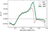 |
Fig. A.1. Relative difference of the squared solar sound speed chelio and the sound speed obtained from models using the Asplund et al. (2009)-abundances cmodel: δc2/c2 = (chelio2 − cmodel2)/chelio2. The solar models using MLT (light blue), the 1KM (light pink), and the 3KM (green) are shown. |
Appendix B: Test of the effects of calibration
The models with different combinations of the free parameters (Sect. 4.2) are calibrated to a lower accuracy than the fiducial model from Sect. 4.1. This is because of the time-consuming calibration process, since only small adjustments can be made in each calibration step due to the difficult convergence of the model. To investigate which effects are caused by a lower accuracy of the calibration, and which are actually caused by the different values for the free parameters of the convection theory, we calculated solar models with a lower accuracy than the fiducial model and compared them. The accuracy of these models and the resulting values of αΠ are given in Table B.1.
Testing the effect of using the abundances from Asplund et al. (2009) (Appendix A), and of models with lower accuracy (Appendix B)
Figure B.1 compares the sound speed profiles of the three models given in Table B.1. The sound speed of the outer layers is heavily influenced by the radius of the model. Because the models were calibrated to a lower accuracy, the difference in the sound speed between the observation and the models with αΠ = 2.2 and αΠ = 2.102 reaches absolute values of ≈0.05 in the outer layers. Compared to the fiducial model, this increases the absolute difference in δc2/c2 by 0.05, and 0.04, for the model with αΠ = 2.102 and αΠ = 2.2, respectively. However, the feature close to the boundary of the convective envelope is less affected, as can be seen in the lower panel of Fig. B.1. In this region, compared to the fiducial model, δc2/c2 is decreased by 3.4 ⋅ 10−4 for the model with αΠ = 2.2, and increased by 4.2 ⋅ 10−4 for the model using αΠ = 2.102.
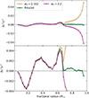 |
Fig. B.1. Relative difference of the squared solar sound speed chelio and the sound speed obtained from models with varying accuracy of the calibration cmodel: δc2/c2 = (chelio2 − cmodel2)/chelio2. The upper panel shows the complete range, while the lower panel zooms in to show more details. |
The difference in Rcz between the models reflects the general difference in the exact radius of the models. The absolute extent of the convective envelope, ΔRcz = Rcz − R★, is barely changed. Compared to the fiducial model, it is increased by 2 ⋅ 10−5 R⊙ for the model with αΠ = 2.102, and decreased by 7 ⋅ 10−5 R⊙ for the model with αΠ = 2.2. Also, the He content of the envelope is not affected (see Table B.1).
Therefore, one can conclude that a lower accuracy of a calibrated solar model will mainly affect the outer parts of the sound speed profile, while the effect on the inner boundary of the convective envelope is minor.
Appendix C: Settings for GYRE
We used the following settings for the control file for GYRE (Townsend & Teitler 2013). If not stated otherwise, we used the default settings. We used the outer boundary conditions and dependent variable set following ADIPLS (Christensen-Dalsgaard 2008). The fourth-order Gauss-Legendre Magnus difference equation scheme was used. For the frequency scan parameters, we used freq_min = 1000, in units of μHz, freq_max = 1 in units of the acoustic cut-off frequency, and n_freq = 100. Furthermore, we used w_ctr = 10, w_osc = 10, w_exp = 4.
All Tables
Testing the effect of using the abundances from Asplund et al. (2009) (Appendix A), and of models with lower accuracy (Appendix B)
All Figures
|
Fig. 1. Relative difference of the squared sound speed of the helioseismic measurement chelio and the solar calibrated models cmodel, using MLT (light blue), 1KM (light pink), and 3KM (green). The quantity on the y-axis is defined as δc2/c2 = (chelio2 − cmodel2)/chelio2. The crosses denote the radii of the data points from the helioseismic inversion. |
| In the text | |
|
Fig. 2. Temperature gradient of the SSM-3KM (green) at the inner boundary of the convective envelope in comparison with the adiabatic (solid black line) and radiative (dashed black line) temperature gradient. The boundary of the convective region as predicted by the model (dotted black line) and as measured by helioseismology (dotted red line) are indicated by vertical lines. The grey shaded regions indicate the 1σ uncertainty of the measurement. The dash-dotted line denotes the radius where ω = 0. The light grey line indicates the temperature profile deduced by Christensen-Dalsgaard et al. (2011). |
| In the text | |
|
Fig. 3. Derivative of the sound speed of the SSM-3KM. The vertical lines denote the boundary of the convective envelope as measured by helioseismology (dotted red) and as predicted by the SSM-3KM (dotted black). The dash-dotted vertical line denotes the radius where ω = 0. The 1σ ranges of the measurement are indicated by the grey shaded region. |
| In the text | |
|
Fig. 4. Temperature stratification of the outer 0.0015 R⊙ of the SSM-3KM. |
| In the text | |
|
Fig. 5. Temperature gradient against the temperature of SSM-MLT (light blue), SSM-1KM (light pink), and SSM-3KM (green). The thick dashed line shows the temperature gradient of the patched model (Jørgensen & Weiss 2019). The temperature range we show corresponds to the outermost 0.0017 R⊙. The inset shows a zoom-in into the region with a negative temperature gradient. |
| In the text | |
|
Fig. 6. Helioseismic surface effect, i.e. the mismatch between the observed frequencies and those calculated from SSM-MLT (light blue), SSM-1KM (light pink), SSM-3KM (green), and the solar model using an averaged 3D atmosphere as the outer boundary condition (“patched model”, black, Jørgensen & Weiss 2019). |
| In the text | |
|
Fig. 7. Pressure against temperature in the uppermost regions. The light pink line shows the profile for SSM-1KM, which largely overlaps the light blue line showing the SSM-MLT. The dashed black line shows the profile of the solar model using an averaged 3D atmosphere as the outer boundary condition (“patched model”, Jørgensen & Weiss 2019). SSM-3KM is represented by the green line. The segment corresponds to the outermost 0.0026 R⊙. |
| In the text | |
|
Fig. 8. Solar models obtained with the 3KM and different sets of free parameters (see Table 1). From left to right, the panels show the difference of the sound speed profile between models and observations, the temperature stratification of the outer layers, and the temperature stratification at the inner boundary of the convective envelope. The vertical lines in the right panels denote the radius at which the change of the slope in the profile of the temperature gradient is strongest. The dotted red line denotes the helioseimisc measurement, with the 1σ ranges indicated by the grey shaded regions. |
| In the text | |
|
Fig. 9. Radius at which the models switch to the local closure relations for the outer regions. Case A is shown in purple. For better visibility, case B (turquoise) and case C (orange) are shifted by –0.001 and –0.0024, respectively (see Table 2). The black lines show ∇ad of the different models, shifted by the same amount as the model ∇. The dotted vertical lines mark the last grid point at which the fully non-local 3KM was applied. |
| In the text | |
|
Fig. 10. Temperature gradient against temperature of the uppermost layers. The temperature range shown corresponds to the uppermost 0.0034 R⊙. The thin light blue and light pink lines show the profiles for SSM-MLT and SSM-1KM, respectively. The dashed black line shows the profile of a solar model using an averaged 3D atmosphere as outer boundary condition (“patched model”, Jørgensen & Weiss 2019). The green, purple, turquoise, and orange lines show the profiles for the fully non-local 3KM, and for case A, case B, and case C, respectively (see Table 2). |
| In the text | |
|
Fig. 11. Surface effect of the solar models with different closure relations for the 3KM in the outer regions (fully non-local: green; case A: purple; case B: turquoise; case C: orange; see Table 2). The result for SSM-MLT (light blue triangles), SSM-1KM (light pink dots), and the patched model (black, Jørgensen & Weiss 2019) are shown for comparison. |
| In the text | |
|
Fig. 12. Hertzsprung-Russel diagram showing the evolution of the solar models. The models using MLT and the 1KM are shown in thin light blue and light pink lines for comparison. The different treatment of the outer layers for the models with 3KM results in higher (Case A: purple) and lower (fully non-local: green; Case B: turquoise; Case C: orange) effective temperatures on the RGB compared to MLT and 1KM. |
| In the text | |
|
Fig. A.1. Relative difference of the squared solar sound speed chelio and the sound speed obtained from models using the Asplund et al. (2009)-abundances cmodel: δc2/c2 = (chelio2 − cmodel2)/chelio2. The solar models using MLT (light blue), the 1KM (light pink), and the 3KM (green) are shown. |
| In the text | |
|
Fig. B.1. Relative difference of the squared solar sound speed chelio and the sound speed obtained from models with varying accuracy of the calibration cmodel: δc2/c2 = (chelio2 − cmodel2)/chelio2. The upper panel shows the complete range, while the lower panel zooms in to show more details. |
| In the text | |
Current usage metrics show cumulative count of Article Views (full-text article views including HTML views, PDF and ePub downloads, according to the available data) and Abstracts Views on Vision4Press platform.
Data correspond to usage on the plateform after 2015. The current usage metrics is available 48-96 hours after online publication and is updated daily on week days.
Initial download of the metrics may take a while.