| Issue |
A&A
Volume 709, May 2026
|
|
|---|---|---|
| Article Number | A101 | |
| Number of page(s) | 12 | |
| Section | Cosmology (including clusters of galaxies) | |
| DOI | https://doi.org/10.1051/0004-6361/202558836 | |
| Published online | 12 May 2026 | |
Integrated Sachs–Wolfe maps from the Gower Street wCDM simulations
1
MTA–CSFK Lendület “Momentum” Large-Scale Structure (LSS) Research Group, Konkoly Thege Miklós út 15-17, H-1121 Budapest, Hungary
2
Konkoly Observatory, HUN-REN Research Centre for Astronomy and Earth Sciences, Konkoly Thege Miklós út 15-17, H-1121 Budapest, Hungary
3
Institute of Physics and Astronomy, ELTE Eötvös Loránd University, Pázmány Péter sétány 1/A, H-1117 Budapest, Hungary
4
Institute for Astronomy, University of Hawaii, 2680 Woodlawn Drive, Honolulu, HI 96822, USA
★ Corresponding author: This email address is being protected from spambots. You need JavaScript enabled to view it.
Received:
31
December
2025
Accepted:
9
March
2026
Abstract
Context. The late-time linear integrated Sachs-Wolfe (ISW) effect directly probes the dynamics of cosmic acceleration and the nature of dark energy. Detecting these weak, secondary temperature anisotropy signals of the cosmic microwave background requires accurate theoretical predictions of their amplitude across cosmological models.
Aims. By extending the pyGenISW package, previously limited to the Lambda cold dark matter (ΛCDM) model, we aim to generate full-sky ISW maps for a suite of 791 wCDM cosmologies using the Gower Street N-body simulations, enabling ISW analyses across a broader dark-energy parameter space. We make our code and ISW data publicly available.
Methods. We computed the ISW signals by tracing the time evolution of the gravitational potential across large-volume simulations that span dark energy equation of state parameters from phantom to quintessence, −1.79 ≲ w ≲ −0.34. These data are projected onto the sphere using HEALP IX to obtain full-sky temperature maps.
Results. We validate our pipeline by comparing the measured ISW angular power spectra and ISW-density cross-correlations against linear theory expectations (2 ≤ ℓ ≤ 200) computed with benchmarks from the pyCCL library. The agreement is excellent across the multipole range where the ISW contribution is expected to dominate, confirming the reliability of our modelling of gravitational-potential evolution. With additional tests of the ISW signal’s strength in density extrema, as well as comparisons of all models to a reference ΛCDM cosmology using power ratios, we find that quintessence-like models (w > −1) show higher ISW amplitudes than phantom models (w < −1), consistent with the enhanced late-time decay of gravitational potentials.
Conclusions. The consistency of our wCDM ISW maps and their agreement with theory predictions confirm the robustness of our methodology, establishing it as a reliable tool for theoretical and observational ISW-LSS analyses. This includes applications to next-generation surveys in the context of covariance calculations and various map-based statistics.
Key words: cosmic background radiation / cosmology: observations / dark energy / large-scale structure of Universe
© The Authors 2026
 Open Access article, published by EDP Sciences, under the terms of the Creative Commons Attribution License (https://creativecommons.org/licenses/by/4.0), which permits unrestricted use, distribution, and reproduction in any medium, provided the original work is properly cited.
This article is published in open access under the Subscribe to Open model. This email address is being protected from spambots. You need JavaScript enabled to view it. to support open access publication.
1. Introduction
The accelerated expansion of the Universe at low redshifts and the corresponding suppression of the growth of cosmic structure due to dark energy are among the most intriguing mysteries in modern cosmology (see e.g. Riess et al. 1998). Combined with cold dark matter (CDM) in the consensus ΛCDM model, a cosmological constant Λ, i.e. the simplest model for dark energy, fits an impressive range of observations at various time- and length scales. Yet, the nature of these dark substances remains unknown, which motivates further research on both theoretical and observational fronts (see e.g. Abdul Karim et al. 2025).
Given the conceptual challenges posed by Λ, i.e. fine-tuning (Weinberg 1989), the cosmic coincidence problem (Steinhardt 2003), and the wide range of theoretical alternatives (i.e. dynamical dark energy, interacting dark sectors, and modified gravity) (see e.g. Odintsov et al. 2025, for review), it is essential to probe cosmic acceleration from every possible angle and with as many independent datasets as possible. Different cosmological probes are sensitive to different physical aspects of dark energy, from background expansion to the large-scale clustering of matter. A coherent picture may only emerge when these perspectives are combined and cross-checked, in line with the strategies of several current and upcoming cosmological sky survey projects (see e.g. Levi et al. 2013; Amendola et al. 2013).
One particular probe of dark energy via the delicate, redshift-dependent balance of structure growth and cosmic expansion is the integrated Sachs-Wolfe (ISW) effect (Sachs & Wolfe 1967). On top of the primary temperature anisotropies from the recombination era, the ISW signal is a secondary anisotropy of the cosmic microwave background (CMB) radiation, offering a unique window on the dynamical properties of cosmic acceleration. On their journey towards our telescopes, CMB photons traverse galaxy superclusters and voids in the cosmic web (see e.g. Nadathur & Crittenden 2016; Kovács et al. 2022a). They experience blueshifts when falling into a potential well of a supercluster and redshifts when exiting it. In contrast, photons experience redshifts when climbing on a potential hill of a void and blueshifts during their descent. If the depth of the potential does not change with time, as in a matter-dominated Einstein-de Sitter Universe, these blueshifts and redshifts cancel out at the linear level (see also Rees & Sciama 1968, for non-linear effects).
However, if the large-scale gravitational potential decays or grows, photons will end up with a net energy shift, resulting in additional CMB temperature perturbations via the ISW effect, generated by the large-scale matter fluctuations at about ∼100 h−1 Mpc scales. This shift arises because the ISW signal accumulates along the line of sight (LOS), corresponding to an integral over the time evolution of the gravitational potential from the last scattering surface to today. When transitioning from matter domination to dark energy domination at approximately z < 1.5, the late-time ISW effect is sourced by the extra space-stretching effects of dark energy, and its detection is of great interest in modern cosmology.
To detect the tiny ISW signal at the ΔTISW ∼ 1 − 10 μK level, one must cross-correlate the large-angle CMB anisotropies with maps of the cosmic large-scale structure. To quantify the results, it is common to introduce an amplitude parameter, AISW, defined operationally in cross-correlation analyses as the scaling between the measured ISW strength and the prediction from a fiducial ΛCDM model:
 (1)
(1)
If the fiducial ΛCDM model were correct, then we would expect AISW ≈ 1, meaning that the observed ISW signal matches the predicted imprint from the decay of gravitational potentials in a Λ-dominated era. Values of AISW that differ from unity indicate one of the following: statistical fluctuations, unaccounted observational or modelling systematics, or deviations from the ΛCDM model in terms of expansion and/or growth history (see e.g. Scháfer 2008; Cai et al. 2014a; Velten et al. 2015; Carbone et al. 2016; Mostaghel et al. 2018; Adamek et al. 2020; Ghodsi Yengejeh et al. 2023, and references therein, for ISW modelling in alternative models).
Traditional detection methods include two-point correlation measurements and cross-power spectra, using increasingly large galaxy catalogues over the last two decades (see e.g. Cooray 2002; Fosalba et al. 2003; Cabré et al. 2007; Giannantonio et al. 2008; Xia et al. 2009; Granett et al. 2009; Dupé et al. 2011; Rassat et al. 2013; Planck Collaboration XXI 2016; Stölzner et al. 2018; Ansarinejad et al. 2020; Bahr-Kalus et al. 2022, and references therein). The majority of these results are consistent with AISW ≈ 1 and thus with the standard ΛCDM model, albeit with low-to-moderate detection significances. As a state-of-the-art result, a recent ISW analysis by Hang et al. (2021b) reported AISW ≈ 0.984 ± 0.349, corresponding to a 2.8σ detection, using the Dark Energy Spectroscopic Instrument (DESI) Legacy Survey galaxy catalogues. This finding is again fully consistent with ΛCDM expectations.
Since the ISW signals are intrinsically weak, a complementary approach involves stacking cutout images of the CMB temperature map at positions of specific large-scale structures, such as voids and superclusters, to target the most extreme parts of the cosmic web where most of the ISW imprints are generated. A series of such stacking analyses on superstructures detected hot (cold) CMB imprints associated with superclusters (voids) identified in galaxy catalogues, pioneered above all by Granett et al. (2008), who reported a ∼4.4σ detection using Sloan Digital Sky Survey (SDSS) data and Wilkinson Microwave Anisotropy Probe (WMAP) CMB data. This was also later confirmed using Planck observations (Planck Collaboration XXI 2016).
These findings were especially intriguing, because theoretical analyses have concluded that the observational ISW signal from superstructures is significantly higher than expected in the standard ΛCDM model (see e.g. Nadathur et al. 2012; Hernández-Monteagudo & Smith 2013; Ilić et al. 2013). Several further studies have revisited and extended this approach:
-
Using galaxy catalogues from the Baryon Oscillations Spectroscopic Survey (BOSS) and the dark energy survey (DES), some results again showed excess ISW signals from the largest voids in particular (see e.g. Cai et al. 2014b; Kovács et al. 2017; Kovács 2018), confirming the findings of Granett et al. (2008) in other sky regions and using alternative void catalogues.
-
In particular, Kovács et al. (2019) found AISW ≈ 5.2 ± 1.6 (3.3σ significance) using R ≥ 100 h−1 Mpc supervoids identified in the BOSS Data Release 12 and DES Year-3 datasets and combined into a joint measurement.
-
Using alternative void finding and stacking techniques applied to the BOSS galaxy catalogues, however, Nadathur & Crittenden (2016) reported no significant tension with AISW ≈ 1.64 ± 0.53.
-
From DESI data, Hang et al. (2021a) reported no significant detection of the stacked ISW signal from voids and found AISW ≈ 1.52 ± 0.72 for superclusters, consistent with no evidence for excess signals.
Beyond stacking methods using hundreds or thousands of voids, the CMB Cold Spot, one of the most extreme anomalies in the CMB, (see e.g. Cruz et al. 2005) and the Eridanus supervoid (Szapudi et al. 2015; Finelli et al. 2015; Kovács & García-Bellido 2016) have also been studied extensively. It has been hypothesized that a large void in the LOS could potentially explain the temperature depression at the Cold Spot (Rudnick et al. 2007), but in a ΛCDM model, there is no real chance to explain the total temperature pattern as an ISW signal (see e.g. Nadathur & Hotchkiss 2015; Naidoo et al. 2016; Mackenzie et al. 2017). Nonetheless, Kovács et al. (2022a) provided evidence for a significant supervoid at z < 0.2 aligned with the Cold Spot, using not only galaxy counts but also weak lensing maps from DES Year-3 dataset (Jeffrey et al. 2021), suggesting a correlation.
As additional probes of the CMB imprints of voids and superclusters, a series of analyses have also measured their CMB lensing convergence (κ) signals (see e.g. Cai et al. 2017; Raghunathan et al. 2020; Vielzeuf et al. 2021; Hang et al. 2021a; Kovács et al. 2022b; Camacho-Ciurana et al. 2024) and reported no significant tensions. A state-of-the-art analysis using DESI luminous red galaxies (LRGs) detected the CMB κ imprint of voids at the 14σ significance level (Aκ ≈ 1.016 ± 0.054), again finding great agreement with ΛCDM model (Sartori et al. 2025).
Further extending the redshift range of the ISW measurement, the following results added intriguing threads to the ISW puzzle:
-
Kovács et al. (2022c) used an extended Baryon Oscillation Spectroscopic Survey (eBOSS) sample of quasi-stellar objects (QSOs) for ISW stacking measurements at high redshifts. They reported a 2.7σ tension with the ΛCDM model, an apparent sign-change at z > 1.5 (AISW ≈ 3.6 ± 2.1 at 0.8 < z < 1.2, and AISW ≈ −8.49 ± 4.4 at 1.9 < z < 2.2).
-
More recently, Hansen et al. (2025) reported a sign-change of the ISW signal in the very local Universe (z < 0.03), i.e. finding hot imprints for local voids and cold imprints for local overdensities.
These recent indications of (moderately significant) excess signals and especially the claims for sign-reversal for the ISW effect in some redshift ranges, if confirmed, would demand careful theoretical modelling to exclude foregrounds or selection effects. Resolving these tensions and anomalies – as well as understanding how ISW signals vary with redshift and scale – requires advances in both observational data and theoretical modelling. On the data side, technological and resource limits impose an upper limit on how much improvement is feasible (see e.g. Afshordi 2004). Although upcoming surveys such as Euclid are highly promising (Euclid Collaboration: Mellier et al. 2025), fully exploiting their datasets will require substantial time and financial investment.
From the modelling perspective, large-volume simulations and efficient pipelines for generating full-sky ISW maps and mock catalogues are crucial (see e.g. Watson et al. 2014; Beck et al. 2018; Castander et al. 2025). They enable validation of analysis methods, provide realistic covariance estimates, and supply predictions across a broad range of cosmological models. In this work, we used the Gower Street (GS, hereafter) suite of simulations – based on the wCDM model (Jeffrey et al. 2025) – to comprehensively study the ISW effect. Our main objective is to create a novel pipeline to reconstruct ISW maps for various cosmologies in GS, enabling (i) precise predictions for the redshift-dependent ISW imprint across a broad range of w from phantom to quintessence domains and (ii) various cross-correlation measurements including two-point functions, stacking, and simulation-based inference.
The paper is organized as follows. In Section 2, we describe our methodology and the implementation of the ISW calculations and map-making. In Section 3, we present our main results, which are then further discussed in Section 4.
2. Methodology and implementation
2.1. Simulation suite
The GS simulation suite consists of 791 full-sky dark matter-only simulations run with PKDGRAV3 (Potter et al. 2017), based on a flat wCDM cosmology spanning −1.79 ≲ w ≲ −0.34. Each simulation uses a box size of L = 1250 h−1 Mpc, with N = 10803, starting from z0 = 49. Outputs consist of 100 light cone files, equally spaced in proper time between z0 and z = 0, at a HEALP IX1 resolution of NSIDE = 2048 (Gorski et al. 2005). We note that each GS simulation uses a distinct random seed for the initial condition generation, enabling tests of cosmic variance effects. The simulation data are publicly available2.
The simulations vary seven cosmological parameters: the matter density parameter Ωm, the amplitude of fluctuations σ8, the scalar spectral index ns, the dimensionless Hubble constant h = H0/100 km s−1 Mpc−1, the physical baryon density Ωb h2, the dark energy equation-of-state (EoS) w, and the total neutrino mass mν. Figure 1 illustrates the spread of the GS simulation suite in the Ωm − σ8 parameter space. Each point corresponds to one of the 791 simulations, colour-coded by the dark energy EoS parameter w, and with marker size proportional to the total neutrino mass, mν. In what follows, we focus on three representative simulations spanning our parameter space (see Table 1 for details):
-
Sim 127, corresponding to the most extreme phantom dark energy model (w ≃ −1.79),
-
Sim 401, highlighting the strongest quintessence dark energy case in GS suite (w ≃ −0.34),
-
Sim 742, an example for a baseline ΛCDM model (w = −1).
In Figure 1, these examples are highlighted with black, unfilled symbols (square, circle, and triangle, respectively) and highlight the broad coverage of the wCDM parameter space in the GS simulation suite.
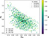 |
Fig. 1. Distribution of the 791 GS simulations in an Ωm − σ8 parameter space, colour-coded by w. The marker sizes illustrate relative differences in neutrino mass. These parameters are the most relevant for ISW calculations. The three representative simulations are highlighted with unfilled black markers. |
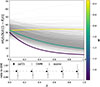 |
Fig. 2. Top panel: Comparison of the ISW kernel, defined as the product of cosmic expansion and growth, for all the 791 GS simulations (grey). We again highlight simulations 401 (yellow), 742 (green), and 127 (dark blue), as representatives of different w values in the GS parameter space. Bottom panel: Our results from the fiducial TheoryCL pipeline and pyCCL compared to alternative computations using CAMB and approximate f(z) formulae described in Section 2.3. This panel highlights the excellent agreement between our pipeline and pyCCL. |
Cosmological parameters for three representative GS simulations, listing additional parameters besides Ωm, σ8, and w (key variables in ISW calculations).
2.2. Integrated Sachs-Wolfe map construction
To generate the ISW temperature maps, we began from the simulated GS light cone catalogues. We used the pyGenISW3 algorithm for the reconstruction of the ISW sky maps from the matter density fluctuations along the LOS (see Naidoo et al. 2021, for further detail). The raw particle counts in each HEALPix pixel were converted into density contrast maps for each light cone slice, which served as the input for pyGenISW.
In addition to the tomographic density maps, we constructed a single density contrast map by merging all simulation light cone slices up to z ≃ 1.0. Later, we used this projected density map for validating our modelling pipeline using galaxy (particle) auto-power spectra and also for computing the ISW-density cross-power spectra.
The pyGenISW algorithm performs a spherical Bessel transform based on a ray-tracing calculation of the ISW temperature anisotropies along the LOS. We created an extended version of the open-source, ΛCDM-compatible version of pyGenISW to properly handle wCDM models and massive neutrinos in GS simulations. In particular, we focused on the linear ISW effect; non-linear contributions – while possible to include via ray tracing – typically modify the signal by only ∼10% (see e.g. Cai et al. 2009). Using these additions, we generated ISW maps up to z ≃ 1.0, where
-
the ISW signal is expected to be strongest in most of the models that we are considering.
-
possible distortions from simulation box repetition effects are expected to be negligible.
-
we expect to have observational data from galaxy surveys to accurately measure these effects in the near future.
2.3. ISW effect in wCDM models
Parallel to the map-based pipeline, we computed theoretical density and ISW power spectra predictions using two independent frameworks: TheoryCL4 (part of the original pyGenISW pipeline, extended here to wCDM cosmologies) and also pyCCL5 for validation against a standard, independent code environment (Chisari et al. 2019). For each simulation, the corresponding set of wCDM cosmological parameters was fed into both theory pipelines to get the expansion and growth histories.
Our starting point is a simple extension of the ΛCDM model, referred to as the wCDM model. It is described by the same six free parameters as the ΛCDM model, with one additional parameter accounting for the total mass of massive neutrinos, and with the dark energy EoS parameter allowed to vary (wDE ≡ w ≠ −1). See Carbone et al. (2016) for further details about the role of w and neutrinos in ISW calculations.
This modifies the Hubble rate through the first Friedmann equation
![Mathematical equation: $$ \begin{aligned} E^2(a) \equiv \dfrac{H^2(a)}{H_{\rm 0}^2} = \left[ \Omega _{\rm m} \, a^{-3} + \Omega _{\rm DE} \, a^{-3 \, (1+w)} \right], \end{aligned} $$](/articles/aa/full_html/2026/05/aa58836-25/aa58836-25-eq2.gif) (2)
(2)
where H0 = 100 h km s−1 Mpc−1 is the Hubble constant, a is the scale factor, and Ωm and ΩDE are the matter and dark energy density parameters, respectively. The physical CDM density parameter is obtained as
 (3)
(3)
where Ωb is the baryon density, and Ων is the neutrino density parameter Lesgourgues & Pastor (2006), Mauland et al. (2023).
The cross-correlation between two statistically isotropic Gaussian fields X and Y can be expressed as
 (4)
(4)
where P(k) is the matter power spectrum today (Manzotti & Dodelson 2014; Stölzner et al. 2018), and IℓX(k) represents the angular transfer (or kernel) function of the field X. We studied the auto- and cross-power spectra between the ISW temperature and the matter distribution from the GS simulation. We begin by describing the ISW temperature anisotropy.
The temperature anisotropy of the late-ISW effect, due to the evolution of the gravitational potential, can be expressed as
 (5)
(5)
where  is the LOS unit vector, r is the comoving radial distance, so
  represent the 3D comoving position vector. τLS is conformal time of the last scattering surface, TCMB = 2.7255 K is the CMB temperature today, and Φ is the gravitational potential, which satisfies the Poisson equation in Fourier space and in Newtonian gauge as
 (6)
(6)
Taking all these into account, the ISW transfer function can be written as
![Mathematical equation: $$ \begin{aligned} I^{ISW}_{\rm \ell }(k) = \dfrac{3\,H^2_{\rm 0}\,\Omega _{\rm m}}{c^2\,k^2} \int \dfrac{\mathrm{d} }{\mathrm{d} z} \left( \dfrac{D(z)}{a(z)} \right) \, j_{\rm \ell } \left[ k_{\rm \chi }(z) \right] \, \mathrm{d} z. \end{aligned} $$](/articles/aa/full_html/2026/05/aa58836-25/aa58836-25-eq9.gif) (7)
(7)
Similarly, the matter (in our case, particles) transfer function is given by
![Mathematical equation: $$ \begin{aligned} I^{g}_{\rm \ell }(k) = \int \dfrac{\mathrm{d} N}{\mathrm{d} z} b(z) \, D(z) \, j_{\rm \ell } \left[ k_{\rm \chi }(z) \right] \, \mathrm{d} z, \end{aligned} $$](/articles/aa/full_html/2026/05/aa58836-25/aa58836-25-eq10.gif) (8)
(8)
where jℓ[kχ(z)] is spherical Bessel function, dN/dz is the redshift distribution function of the sources, b(z) is the linear, scale-independent galaxy bias (in our case b(z) = 1 because we work with dark matter particles), and D(z) is the linear growth factor. Although the Limber approximation is available in the original implementation of TheoryCL, it was not used in this study. Instead, we evaluated the full expressions above, retaining the spherical Bessel functions, which is particularly important for the low-multipole regime relevant to the ISW effect.
In practical terms, we calculated a simple combination of the expansion rate, H(z), and growth histories, D(z) and f(z) = dlnD/dlna, often referred to as the ISW kernel:
![Mathematical equation: $$ \begin{aligned} \Delta T^\mathrm{ISW} \sim \dot{\Phi } \sim D(z) \, H(z) \, \left[ 1 - f(z) \right]. \end{aligned} $$](/articles/aa/full_html/2026/05/aa58836-25/aa58836-25-eq11.gif) (9)
(9)
Linear matter density perturbations grow as δ(r, z) = D(z)δ(r) and ∇2Φ(r, z) = (3/2)H02Ωm δ(r, z)/a. By combining linear growth and the Poisson equation, it follows that ![Mathematical equation: $ \dot{\Phi}=-H(z)[1-f(z)]\Phi $](/articles/aa/full_html/2026/05/aa58836-25/aa58836-25-eq12.gif) .
.
In our pipeline (see Figure 3), we implemented three complementary methods to compute the linear growth factor and growth rate. Although all three options are available to users, our fiducial choice throughout this work is the ordinary differential equation (ODE)-based solution.
-
The ODE approach (fiducial): In this method, the linear growth factor is governed by solving the standard differential equation for matter perturbation in a homogeneous and isotropic Universe:
 (10)
(10)This is the baseline approach adopted throughout the paper, and we find excellent agreement with the pyCCL predictions for the GS simulation (which also uses an ODE method for growth calculations). Once DODE(z) is obtained, the linear growth rate is computed as
 (11)
(11)In this method, the effect of massive neutrinos enters solely through the background term of Ων defined in Equation (3), while their scale-dependent clustering is not included in the perturbation equation. We note that in the linear regime where the ISW effect is strongest, and for neutrino mass ranges considered in the GS simulations, the expected additional ISW temperature perturbations by neutrinos are negligible (see e.g. Cuozzo et al. 2024).
-
CAMB-based approach: As an alternative to solving the growth equation directly, we obtained the linear growth factor from the Boltzmann code CAMB6. It computes the full linear matter power spectrum, Plin(k, z), including the scale-dependent suppression induced by massive neutrinos. To extract the growth factor, we followed the standard convention of using the redshift evolution of the root mean square (RMS) of linear matter density fluctuations on 8 h−1 Mpc scales,
 (12)
(12)Here, σ8(z) is obtained by integrating the linear matter power spectrum over wave number, yielding an effective, scale-averaged amplitude of fluctuations. Even though Plin(k, z) is scale-dependent, the resulting DCAMB(z) remains scale-independent. In our implementation of this method, the growth rate, f(z), is not provided directly by CAMB; instead, the pipeline computes it numerically, by differentiating the tabulated D(z) values, evaluating f(z) = dlnD/dlna directly from the discrete D(z) grid.
-
Analytic approximation approach: For fast evaluations, the pipeline also includes the well-known growth-index approximation, in which the growth rate is parametrized as
 (13)
(13)where γ(w) is the growth index (Linder 2005). In the context of wCDM cosmologies, it is approximated by
 (14)
(14)This approximation is computationally efficient, but its accuracy degrades for models when w deviates significantly from −1, or in models with more complex growth behaviour. Users should therefore verify its suitability for their parameter space. In this approach, the pipeline computes the growth factor using the CAMB-based method. This hybrid approach ensures a stable and accurate D(z) while retaining the speed of the analytic growth-rate approximation.
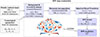 |
Fig. 3. Simulation-based ISW map construction. Density contrast maps and cosmological parameters from the GS simulation are propagated through a unified model (extended TheoryCL) and a spherical-Bessel ISW pipeline (extended pyGenISW), yielding fully consistent ISW power spectrum predictions and corresponding ISW temperature maps. |
2.4. Mapmaking with pyGenISW
Given the expansion and growth functions, the next step in the pipeline is to construct the underlying 3D density field ζ(χ, θ, ϕ) to compute the ISW temperature anisotropies. The density field is expanded in a basis that is adapted to the spherical geometry of the light cone with a finite radial range, where χ denotes the comoving distance from the observer.
We employed the discrete spherical-Bessel transform (SBT) using pyGenISW, which provides an orthonormal set of radial eigenfunctions on a finite space χ ∈ [0, χmax]. In this domain, the free eigenfunctions are jℓ[kℓn χ], directly analogous to the jℓ[kχ(z)] terms appearing in the ISW and matter transfer functions. We imposed a Neumann boundary condition at the edge of the light cone,
 (15)
(15)
which defines the allowed discrete radial modes
 (16)
(16)
where qℓn is the n-th zero of ∂xjℓ(x). Using this discrete set of radial wave numbers, we created the ISW temperature map through the following steps:
-
Expanding the density field in the spherical Fourier-Bessel (SFB) basis to obtain the coefficients δℓmn.
-
Projecting Equation (6) onto the SFB basis and replacing the continuous wave number k with the discrete modes kℓn in Equation (16) to obtain the SFB coefficients of the potential
 (17)
(17) -
Reconstructing the potential in harmonic space by summing over the radial modes:
 (18)
(18) -
Taking the spherical harmonic transform of Equation (5) and expressing the potential in the SFB basis, where the ISW harmonic coefficients can be written as
 (19)
(19) -
Reconstructing the ISW map from the harmonic coefficients via
 (20)
(20)
The expression for  forms the starting point for the radial kernel formulation given in Eq. (33) of Naidoo et al. (2021), where the ISW signal is written as a weighted radial projection of the SFB density coefficients. However, in our implementation, the weighting was explicitly performed along the LOS, consistent with the definition of the ISW effect as an integral along the photon path, rather than using a volume-based weighting.
In practice, the coefficients δℓmn were obtained by projecting the simulated density field onto the discrete spherical Bessel basis, and the ISW harmonic coefficients  were then evaluated using the expression above and transformed into a temperature map via an inverse spherical harmonic transform (using alm2map). To ensure consistency with the map-making pipeline, all theoretical calculations use the galaxy (in our case, particle) redshift distribution, N(z), measured directly from the simulation light cones. From these maps and kernels, we computed the ISW auto-power spectrum, the density auto-power spectrum, and the ISW-density cross-power spectrum.
Computationally, this pipeline follows the method introduced by Naidoo et al. (2021), extended with additional cosmological parameters as input arguments. It allows for a user-selected prescription of the linear growth rate, f(z), and the corresponding growth factor, D(z), using three alternative approaches described in Section 2.3: a direct numerical solution of the growth equation (ODE approach), a Boltzmann-solver-based (CAMB-based approach), or an analytic approximation approach. We also modified the radial window function normalization, created alternative treatments of slice-effective radii, improved numerical integration routines (Simpson instead of trapezoidal), and enhanced the spherical harmonic pipeline that incorporates pixel-window deconvolution, which is handled within the pyGenISW-based code.
3. Results
3.1. Validation of the theoretical framework
Before computing the wCDM ISW maps, we first validated the theoretical framework by examining the redshift evolution of the ISW kernel in the linear regime. The growth factor and growth rate, obtained from the extended TheoryCL pipeline, feed directly into the ISW kernel, defined in Equation (9) (see e.g. Cai et al. 2009). This allowed us to verify that our pipeline correctly captured the expected dependency on cosmological parameters.
The top panel of Figure 2 shows the redshift evolution of the ISW kernel in linear theory, where curves cover the interval 0 ≤ z ≤ 1, consistent with the redshift range of the ISW maps created in this work (limited by box repetition effects). We display results from all of our ODE-based, extended TheoryCL computations in grey, spanning the full range of cosmologies sampled by the GS simulations, colour-coded according to their w values.
The bottom panel in Figure 2 shows the ratio of several alternative growth-rate prescriptions to the ODE-based calculation. We compare results from pyCCL (black), the CAMB-based growth factor (light grey), and the analytic approximation method (grey). Their ratios are evaluated at five representative redshifts, and each data point represents the mean over 791 simulations, with error bars showing the corresponding standard deviation.
We identify several trends. First, the ODE approach of TheoryCL kernel agrees extremely well with pyCCL across all redshifts, as expected since both packages solve the same underlying differential equation. In contrast, the CAMB-based values show systematic deviations of up to 2% at high redshift, with a growing offset from the central value of unity, and the error bars also increase with z. The analytic approximation shows somewhat larger scatter at all redshifts, though its 1σ error bars overlap with unity for z ≳ 0.3. Overall, Figure 2 highlights the robustness and reliability of our TheoryCL ODE approach, yielding ISW kernel predictions that are fully consistent with those from the widely used pyCCL framework for all wCDM cosmologies in our sample.
3.2. ISW map statistics
For 777 of the 791 GS mocks, we managed to create an ISW map using our extended pyGenISW pipeline. In the remaining 14 simulations, we identified numerical instabilities or convergence issues that prevented reliable ISW map generation. In Figure 4, we show three representative ISW maps generated with our pipeline. As expected, the overall ISW fluctuation power is strongest for Sim 401 with w = −0.34 (determined by a consistently strong kernel values up to high redshifts, see again Figure 2). In line with our expectations, Sim 742 ranks second in the ISW signal strength, and then Sim 127 features the weakest overall ISW pattern, due to a later onset of the dark energy component with w = −1.79. We note that we removed the ℓ < 10 modes from the ISW maps, for better visualization of the largest scales that we can certainly reconstruct with the GS simulations, given their box size.
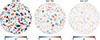 |
Fig. 4. Sky-maps of the ISW signal, showing half of the sky in an orthographic projection. Three representatives correspond to simulations 401 (w = −0.34), 742 (w = −1), and 127 (w = −1.79), which highlight different dark energy EoS. These maps are colour-coded based on the ISW temperature anisotropies in μK. The quintessence model shows the most pronounced colours, indicating the strongest ISW signal, followed by the ΛCDM model, while the phantom model shows the weakest signal (see also Figure 5 for comparison). |
In Figure 5, we also illustrate the ISW signal contributions from different redshift ranges in these three simulations with different w values. At low redshift (z < 0.2), all models have nearly identical histograms despite their remarkably different values of w. But we should consider that w is not the only relevant cosmological parameter here (see Table 1 for a complete list), especially when it comes to the low-redshift regime. We calculated the ISW map fully in the linear regime, and the growth rate of linear gravitational potentials is already low at the present epoch. This is controlled primarily by Ωm, which in our three simulations varies only up to ∼8% level between Sim 127 and Sim 401. On the other hand, Sim 742 has the highest σ8 around 10% higher than Sim 127, which can compensate for the differences caused by w. As a result, the models become distinguishable only at intermediate redshifts where the ISW kernel reaches its maximum sensitivity to the growth history. We make the following observations:
-
From z ≈ 0.3 onward, differences become more visible, when the phantom model (Sim 127) generally produces narrower and sharper distributions, indicating smaller ISW signals, while the quintessence model (Sim 401) shows broader and shallower distributions, reflecting larger temperature fluctuations.
-
The strongest separation occurs around 0.6 < z < 1.0. Because the horizontal axis shows temperature fluctuations in μK around zero, a sharper histogram corresponds to a weaker overall signal. In this intermediate interval, the quintessence model (Sim 401) shows the broadest distribution, showing the strongest ISW fluctuations among the three representatives in these redshift bins, consistent with the fact that in a quintessence-like cosmology, matter-Λ equality occurs at a higher redshift (earlier time) than in phantom models for the same present-day densities.
-
In the final panel for the entire redshift interval considered in GS, 0.0 < z < 1.0, the ordering of peaks with the highest for the phantom model reflects the cumulative effects induced by different dark energy EoS.
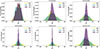 |
Fig. 5. Histograms of ISW temperature maps for the three characteristic examples: Sim 127 (w = −1.79), Sim 742 (w = −1), and Sim 401 (w = −0.34). The different panels show the redshift-binned ISW temperature statistics using HEALP IX pixel values. Clear trends are visible with varying w parameters and also with redshift. |
In line with this, most current and upcoming surveys (e.g. Euclid, Rubin-LSST, and DESI) provide their highest signal-to-noise measurements of galaxies in this redshift range. Our simulated ISW maps will provide a new environment for covariance estimation and higher-order statistical modelling tools to fully extract the joint LSS-CMB information from these surveys. While the current GS suite contains more than 700 realizations, they span a wide range of cosmological parameter combinations. Therefore, they do not represent the covariance matrix of a fixed fiducial cosmology and are not suitable for likelihood in cross-correlation at this stage. A dedicated study using multiple realizations at fixed cosmology will be investigated in future work, using other sets of GS simulations.
3.3. Simulation-based versus theoretical power spectra
In Figure 6, we show the ISW auto-power spectrum,  in the left panel, over the multipole range 2 ≤ ℓ ≤ 200, again for the three representative simulations. For each model, we compare the theoretical predictions from TheoryCL with the power spectrum measurements using the anafast7 method, estimated from our pyGenISW-based ISW maps. Both sets of curves are logarithmically binned to suppress small-scale fluctuations and to emphasise the large-scale behaviours. The colour-coded shaded regions indicate the 1σ cosmic variance band derived from the TheoryCL predictions as
 (21)
(21)
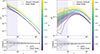 |
Fig. 6. Theoretical vs. map-based power spectra for ISW auto-correlations (left) and galaxy auto-correlations (right). Top panels: Three characteristic models with different w parameters, comparing the measured value from pyGenISW and anafast (solid) with the theoretical expectations from TheoryCL (dashed). We mark the limitations due to cosmic variance (shaded about dashed lines) and also the ℓ < 10 range where we expect to have imperfect density and ISW maps due to the GS box size limitations. Bottom panels: Statistical results for the agreement of the fiducial TheoryCL and alternative pyCCL theoretical pipelines, and also a comparison between theory and map-based results for the ensemble of the GS mocks. We report good agreement, with a slight deficit of power at small scales (ℓ ≥ 100) where the ISW signal is weakest, and where linear theory assumptions might break down first. |
where fsky is the observed sky fraction (in our case 1) and Cℓ is the angular power spectrum.
Creating a summary statistic for the performance of our ISW map-making pipeline using all the GS simulations, the bottom panel shows the ratio between map-based results from pyGenISW (grey points) and from pyCCL (black points) and the TheoryCL predictions. We cannot expect a perfect match simply due to cosmic variance limitations, but we ensured an excellent statistical match for the 777 correctly processed mocks. For reference, the 1σ cosmic variance based on the TheoryCL spectrum is also shown, displaying the expected imperfections for a single map. The points and error bars in the bottom panel represent the mean and standard deviation of the ratios over all 777 simulations, for each of the ten logarithmic bins.
In both panels, ℓ < 10 are visually shaded to highlight the limitations imposed by the finite simulation volume. To create a full sky light cone from repeated simulation boxes, modes larger than the box size are not independent, leading to artificial large-scale power and unreliable estimates in these multipoles. Furthermore, we also note that in typical ISW measurements, these modes are often removed from the analysis due to possible biases due to masking, and considering that these scales are much larger than the typical angular size of voids and superclusters (see e.g. Kovács et al. 2020).
The right column of Figure 6 shows the galaxy auto-power spectrum,  , which does not contain any ISW contribution. For the pyGenISW-based measurements, we obtain it directly from the merged density-contrast maps, constructed by stacking all light cone slices up to z ≃ 1.0, and compute the harmonic-space spectrum using anafast. The corresponding theoretical predictions from TheoryCL and pyCCL use the simulated N(z) as explained above. Apart from the physical quantity being plotted, the treatment is identical to the left column. We again find great agreement between theoretical and map-based power spectra, except at ℓ < 10 where the GS simulations become insufficient to accurately model the matter density fluctuations due to box-size effects.
This can be understood quantitatively from the fundamental mode of the simulation box. In Fourier space, the largest mode that we can estimate is kB = 2π/LB. Considering our box size where LB = 1250 Mpc h−1 indicating that the GS simulations cannot represents modes with kB < 0.005 Mpc h−1. One can use the Limber approximation to connect 3D scales to angular scales, ℓ ∼ k χ(z). For the redshift range where most of the ISW signals come from (zeff ∼ 0.3 − 1.0) the corresponding comoving distance range is roughly 800 − 2300 Mpc h−1, implying ℓB ∼ 4 − 11. Therefore, a suppression of power is expected below ℓ ≃ 10 for the GS simulations.
In Figure 7, we also show our results for the ISW-galaxy cross-power spectrum statistics. We again report good agreement between the two theoretical pipelines. Theoretical and map-based power spectra are in close match when looking at individual simulations and cosmic variance limits, or when considering the overall ensemble-average statistics for the 777 GS mocks.
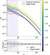 |
Fig. 7. Similar to Figure 6, but for the galaxy-ISW cross-correlation. Different simulations with varying w parameters show different power spectrum amplitudes, and the overall agreement is great between theory and map-based results, except for the lowest and highest ℓ-ranges. |
Overall, we report great agreement between theoretical expectations and the properties of the ISW temperature maps that we generated for the GS simulations, in an extended wCDM parameter space. The largest scales at ℓ < 10, and the smallest scales at ℓ ≥ 100 are where we find some power deficit in the maps, also in the ensemble averages given their standard deviations. However, these features in  ,
,  , and
, and  originated from box-size and resolution effects that are expected consequences of our input simulations and our methodology, and they remain at the ∼1 − 2σ level.
3.4. ISW signals in density extrema
We also tested the role of the input cosmology by splitting the δm projected matter density field into percentiles, i.e. identifying troughs and peaks where the ISW is expected to be maximal (see e.g. Gruen et al. 2016). To reduce small-scale fluctuations in the map, we applied a σ = 5° Gaussian smoothing to the density field, while from the ISW map we again removed ℓ < 10 modes.
For a random subset of 50 wCDM simulations, we measured the mean ΔTISW temperatures in each density-split bin defined in the HEALP IX maps. Providing an example for map-level applications of our GS ISW products, these results are summarized in Figure 8. As expected, we found that the magnitude of the ISW signal is enhanced in density extrema, and it shows a clear dependence on the underlying dark energy model. In particular, the quintessence model (Sim 401), shows the largest temperature shifts in both the most overdense and underdense regions, reaching to ΔTISW ∼ ±15 μK, while the phantom model (Sim 127), displays a weaker signal ΔTISW ∼ ±5 μ K. This is also consistent with the results shown in Figure 5. When we apply observational data from galaxy surveys, such measurements could provide complementary constraints to traditional two-point statistics, particularly by exploiting the enhanced signal in voids and clusters.
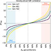 |
Fig. 8. Mean ΔTISW temperatures in percentiles of the δm projected matter density field. The impact of varying the input cosmological parameters is shown here in the most extreme parts of the density field, where the ISW signals differ most (in blue and red shaded areas). |
3.5. ISW power ratios in different models
We further quantified the relative strength of the ISW signal in different models. As introduced in Section 1, the AISW parameter is usually defined as the ratio of the ISW signal measured from data, and a prediction from a fiducial ΛCDM model (Equation (1)). Along similar lines, we computed for all GS models the following ISW power ratio
![Mathematical equation: $$ \begin{aligned} A_{\rm ISW}^{Tg} = \left\langle \frac{\bar{C}^{\, \mathrm{Tg},\, \mathrm{sim} }_{ \ell }}{\bar{C}^{\, \mathrm{Tg}, \,\mathrm{fid} }_{ \ell }} \right\rangle _{[\ell _{\min }, \, \ell _{\max }]}, \end{aligned} $$](/articles/aa/full_html/2026/05/aa58836-25/aa58836-25-eq32.gif) (22)
(22)
with cross-power spectrum  , using Sim 742 as our reference, fiducial ΛCDM model. Given the limitations of our GS methodology, we calculated the above power ratio in the multipole range 10 ≤ ℓ ≤ 200.
Therefore, we did not fit a field-level ISW amplitude or power spectrum template, but we instead compressed the ISW information into a single scalar quantity, the power ratio  , by comparing the overall normalization of the angular power spectra. Figure 9 shows the resulting ISW amplitudes,
  as a function of the matter density parameter, Ωm, for all 777 valid GS simulations. The points are colour-coded by the dark energy EoS parameter, w, and three representative simulations are highlighted with different markers. We make the following observations:
-
The horizontal dashed line indicates the fiducial ΛCDM expectation at
 , among a set of models spanning more than an order of magnitude, reflecting the sensitivity of the ISW effect to late-time cosmological evolution across our wCDM parameter space. The inset histogram shows the distribution of
  .
. -
The wide extent of the distributions with about
 reflects the diversity of cosmological models in the simulation suite. In particular, the broad ranges in parameters such as Ωm and w lead to large variations in the evolution of the late-time gravitational potential.
 -
We note that wCDM models with w > −1 and low values of Ωm produce ISW amplitudes that are consistent with the observed AISW ≈ 5 from some low-z voids. However, no model analysed in this work can explain the apparent sign-change at z < 0.1 and z > 1.5 in void stacking analyses.
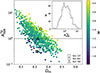 |
Fig. 9. ISW amplitude |


4. Discussion and conclusions
In this work, we developed and validated a novel framework for generating ISW temperature maps for a set of 777 wCDM cosmological models in the GS simulation suite (Jeffrey et al. 2025). In particular, we modified and extended the ΛCDM-compatible pyGenISW temperature map reconstruction methodology (Naidoo et al. 2021) to enable accurate and robust modelling of the ISW signal in a wide range of wCDM models. Our main results are the following:
-
In our validation tests, we compared our theoretical predictions for the
 ,
,  , and
, and  auto- and cross-power spectra with multiple alternatives. The ODE approach to modelling the growth factor provides robust results, consistent with those obtained from the widely adopted pyCCL across the entire 0 ≤ z ≤ 1 redshift interval most relevant to ISW.
 -
Using this framework, we analysed a suite of simulations spanning a wide range of constant w models, including some extreme phantom (w = −1.79) and quintessence (w = −0.34) cases. The ISW auto-power spectra extracted from our pyGenISW maps show excellent agreement with theoretical predictions, when compared in logarithmic multipole bins over 2 ≤ ℓ ≤ 200. The residuals lie well within the expected cosmic-variance envelope for all simulations. At the largest angular scales (ℓ < 10), the discrepancies follow the expected behaviour due to the finite volume of the GS simulations and the associated lack of independent large-scale modes.
-
We further verified that the
 galaxy auto-power spectra derived from the simulated density maps are in agreement with TheoryCL (and pyCCL) predictions when adopting the corresponding N(z) distributions of the GS simulations.
 -
The ISW temperature map histograms evaluated in redshift bins show that all three highlighted cosmologies with radically different w parameters (w = −1.79, w = −1, w = −0.34) remain nearly indistinguishable at very low redshift. This finding indicates that the similar present-day decay rate of gravitational potentials is mostly set by their Ωm values. More noticeable differences only emerge at z ≥ 0.2, where the ISW signal is more sensitive to the growth history.
-
However, integration over the full redshift interval considered in this GS analysis (up to z ≃ 1) distinguishes the three models. We measure the following standard deviations in the ISW maps σΔTISW ≈ 4.99 μK for Sim 127, σΔTISW ≈ 12.12 μK for Sim 742, and σΔTISW ≈ 16.47 μK for Sim 401 (see Figure 5 for detail). This increased variance in the map as a result of lower w values confirms that the ISW signal has contributions across a wide range of cosmic epochs rather than solely from the very local Universe.
-
Testing the extrema, we also split the projected matter density field into percentiles and thus identified extreme troughs and peaks with presumably strong local ISW signals in our maps. As expected, we find that the quintessence model (Sim 401) shows the largest temperature shifts in both the most overdense and underdense regions, while the phantom model (Sim 127), displays a weaker signal than the reference ΛCDM model (Sim 742).
-
Computing power ratios from CℓTg, we estimated
 for all 777 GS simulations, all compared to a fiducial ΛCDM model. The resulting scatter, shown in Figure 9, reflects the combined influence of multiple cosmological parameters. While there is no simple monotonic trend with w, simulations with comparable Ωm values suggest that quintessence-like models (w > −1) tend to exhibit slightly higher ISW amplitudes than phantom-like models (w < −1), consistent with enhanced late-time decay of gravitational potentials.
 -
Taken together, these results from the GS simulations demonstrate that our wCDM ISW maps are both accurate and internally consistent. They provide reliable predictions for the ISW signal’s cosmological dependence in a wide range of models beyond ΛCDM.
Our methodology robustly models the two-point statistics of ISW maps, and our map-based approach also paves the way for higher-order statistics. In subsequent analyses, we will use the density and ISW maps for various cross-correlation measurements – including stacking methods and simulation-based inference – to search for optimal ways to detect deviations from the ΛCDM model via the ISW effect. We also plan to extend this analysis to w0waCDM and perhaps other alternative models, which may offer new insights about dark energy’s dynamical properties using exquisite data from surveys such as Euclid, DESI, Rubin-LSST, and Roman in the coming years.
In the context of possible ISW sign-changes at specific redshift ranges, a robust assessment of whether evolving dark energy models (e.g. w0waCDM) can accommodate such signals requires a dedicated simulation suite and can be investigated in future work. In principle, such a feature could arise from a non-standard gravitational potential evolution – including non-linear structure formation or more exotic dark energy and dark matter physics, potentially in combination – but not within the linear wCDM modelling framework investigated here.
Acknowledgments
The authors thank Barbara Matécsa for assistance with preliminary tests. We also thank Krishna Naidoo, whose work formed the foundation of this paper and who provided valuable guidance and assistance throughout our research. We also thank Susan Pyne and the anonymous reviewer for constructive comments on the manuscript. The Large-Scale Structure (LSS) research group at Konkoly Observatory has been supported by a Lendület excellence grant by the Hungarian Academy of Sciences (MTA). This project has received funding from the European Union’s Horizon Europe research and innovation programme under the Marie Skłodowska-Curie grant agreement number 101130774. Funding for this project was also available in part through the Hungarian National Research, Development and Innovation Office (NKFIH, grant OTKA NN147550). M.G.Y. was supported by the EKÖP-25 University Excellence Scholarship Program of the Ministry for Culture and Innovation from the source of the National Research, Development and Innovation Fund. IS acknowledges NASA grant 80NSSC24K1489. The GS simulations were generated under the DiRAC project p153 ‘Likelihood-free inference with the Dark Energy Survey’ (ACSP255/ACSC1) using DiRAC (STFC) HPC facilities (www.dirac.ac.uk). We are grateful for the possibility to use HUN-REN Cloud (see Héder et al. 2022; https://science-cloud.hu/), which helped us achieve the results published in this paper.
References
- Abdul Karim, M., Aguilar, J., Ahlen, S., et al. 2025, Phys. Rev. D, 112, 083514 [Google Scholar]
- Adamek, J., Rasera, Y., Corasaniti, P. S., & Alimi, J.-M. 2020, Phys. Rev. D, 101, 023512 [NASA ADS] [CrossRef] [Google Scholar]
- Afshordi, N. 2004, Phys. Rev. D, 70, 083536 [Google Scholar]
- Amendola, L., Appleby, S., Bacon, D., et al. 2013, Liv. Rev. Relat., 16, 6 [Google Scholar]
- Ansarinejad, B., Mackenzie, R., Shanks, T., & Metcalfe, N. 2020, MNRAS, 493, 4830 [Google Scholar]
- Bahr-Kalus, B., Parkinson, D., Asorey, J., et al. 2022, MNRAS, 517, 3785 [CrossRef] [Google Scholar]
- Beck, R., Csabai, I., Rácz, G., & Szapudi, I. 2018, MNRAS, 479, 3582 [NASA ADS] [CrossRef] [Google Scholar]
- Cabré, A., Fosalba, P., Gaztañaga, E., & Manera, M. 2007, MNRAS, 381, 1347 [CrossRef] [Google Scholar]
- Cai, Y.-C., Cole, S., Jenkins, A., & Frenk, C. 2009, MNRAS, 396, 772 [Google Scholar]
- Cai, Y.-C., Li, B., Cole, S., Frenk, C. S., & Neyrinck, M. 2014a, MNRAS, 439, 2978 [NASA ADS] [CrossRef] [Google Scholar]
- Cai, Y.-C., Neyrinck, M. C., Szapudi, I., Cole, S., & Frenk, C. S. 2014b, ApJ, 786, 110 [NASA ADS] [CrossRef] [Google Scholar]
- Cai, Y.-C., Neyrinck, M., Mao, Q., et al. 2017, MNRAS, 466, 3364 [NASA ADS] [CrossRef] [Google Scholar]
- Camacho-Ciurana, G., Lee, P., Arsenov, N., et al. 2024, A&A, 689, A171 [NASA ADS] [CrossRef] [EDP Sciences] [Google Scholar]
- Carbone, C., Petkova, M., & Dolag, K. 2016, JCAP, 2016, 034 [CrossRef] [Google Scholar]
- Castander, F. J., Fosalba, P., Stadel, J., et al. 2025, A&A, 697, A5 [Google Scholar]
- Chisari, N. E., Alonso, D., Krause, E., et al. 2019, ApJS, 242, 2 [Google Scholar]
- Cooray, A. 2002, Phys. Rev. D, 65, 103510 [Google Scholar]
- Cruz, M., Martínez-González, E., Vielva, P., & Cayón, L. 2005, MNRAS, 356, 29 [CrossRef] [Google Scholar]
- Cuozzo, V., Carbone, C., Calabrese, M., Carella, E., & Migliaccio, M. 2024, J. Cosmol. Astropart. Phys., 2024, 073 [Google Scholar]
- Dupé, F.-X., Rassat, A., Starck, J.-L., & Fadili, M. J. 2011, A&A, 534, A51 [NASA ADS] [CrossRef] [EDP Sciences] [Google Scholar]
- Euclid Collaboration (Mellier, Y., et al.) 2025, A&A, 697, A1 [Google Scholar]
- Finelli, F., García-Bellido, J., Kovács, A., Paci, F., & Szapudi, I. 2015, MNRAS, 455, 1246 [Google Scholar]
- Fosalba, P., Gaztañaga, E., & Castander, F. J. 2003, ApJ, 597, L89 [Google Scholar]
- Ghodsi Yengejeh, M., Fakhry, S., Firouzjaee, T. J., & Fathi, H., 2023, Phys. Dark Universe, 39, 101144 [Google Scholar]
- Giannantonio, T., Scranton, R., Crittenden, R. G., et al. 2008, Phys. Rev. D, 77, 123520 [Google Scholar]
- Gorski, K. M., Hivon, E., Banday, A. J., et al. 2005, ApJ, 622, 759 [Google Scholar]
- Granett, B. R., Neyrinck, M. C., & Szapudi, I. 2008, ApJ, 683, L99 [NASA ADS] [CrossRef] [Google Scholar]
- Granett, B. R., Neyrinck, M. C., & Szapudi, I. 2009, ApJ, 701, 414 [Google Scholar]
- Gruen, D., Friedrich, O., Amara, A., et al. 2016, MNRAS, 455, 3367 [Google Scholar]
- Hang, Q., Alam, S., Cai, Y.-C., & Peacock, J. A. 2021a, MNRAS, 507, 510 [NASA ADS] [CrossRef] [Google Scholar]
- Hang, Q., Alam, S., Peacock, J. A., & Cai, Y.-C. 2021b, MNRAS, 501, 1481 [Google Scholar]
- Hansen, F. K., Lambas, D. G., Ruiz, A. N., Toscano, F., & Pereyra, L. A. 2025, A&A, submitted [arXiv:2506.08832] [Google Scholar]
- Héder, M., Rigó, E., Medgyesi, D., et al. 2022, Információs Társadalom, 22, 128 [Google Scholar]
- Hernández-Monteagudo, C., & Smith, R. E. 2013, MNRAS, 435, 1094 [CrossRef] [Google Scholar]
- Ilić, S., Langer, M., & Douspis, M. 2013, A&A, 556, A51 [NASA ADS] [CrossRef] [EDP Sciences] [Google Scholar]
- Jeffrey, N., Gatti, M., Chang, C., et al. 2021, MNRAS, 505, 4626 [NASA ADS] [CrossRef] [Google Scholar]
- Jeffrey, N., Whiteway, L., Gatti, M., et al. 2025, MNRAS, 536, 1303 [Google Scholar]
- Kovács, A. 2018, MNRAS, 475, 1777 [CrossRef] [Google Scholar]
- Kovács, A., & García-Bellido, J. 2016, MNRAS, 462, 1882 [Google Scholar]
- Kovács, A., Sánchez, C., García-Bellido, J., & the DES collaboration 2017, MNRAS, 465, 4166 [CrossRef] [Google Scholar]
- Kovács, A., Sánchez, C., García-Bellido, J., & the DES collaboration 2019, MNRAS, 484, 5267 [CrossRef] [Google Scholar]
- Kovács, A., Beck, R., Szapudi, I., et al. 2020, MNRAS, 499, 320 [Google Scholar]
- Kovács, A., Jeffrey, N., Gatti, M., et al. 2022a, MNRAS, 510, 216 [Google Scholar]
- Kovács, A., Vielzeuf, P., Ferrero, I., et al. 2022b, MNRAS, 515, 4417 [CrossRef] [Google Scholar]
- Kovács, A., Beck, R., Smith, A., et al. 2022c, MNRAS, 513, 15 [CrossRef] [Google Scholar]
- Lesgourgues, J., & Pastor, S. 2006, Phys. Rept., 429, 307 [NASA ADS] [CrossRef] [Google Scholar]
- Levi, M., Bebek, C., Beers, T., et al. 2013, arXiv e-prints [arXiv:1308.0847] [Google Scholar]
- Linder, E. V. 2005, Phys. Rev. D, 72, 043529 [Google Scholar]
- Mackenzie, R., Shanks, T., Bremer, M. N., et al. 2017, MNRAS, 470, 2328 [NASA ADS] [CrossRef] [Google Scholar]
- Manzotti, A., & Dodelson, S. 2014, Phys. Rev. D, 90, 123009 [Google Scholar]
- Mauland, R., Elgarøy, Ø., Mota, D. F., & Winther, H. A. 2023, A&A, 674, A185 [NASA ADS] [CrossRef] [EDP Sciences] [Google Scholar]
- Mostaghel, B., Moshafi, H., & Movahed, S. M. S. 2018, MNRAS, 481, 1799 [Google Scholar]
- Nadathur, S., & Crittenden, R. 2016, ApJ, 830, L19 [CrossRef] [Google Scholar]
- Nadathur, S., & Hotchkiss, S. 2015, MNRAS, 454, 889 [NASA ADS] [CrossRef] [Google Scholar]
- Nadathur, S., Hotchkiss, S., & Sarkar, S. 2012, JCAP, 6, 42 [Google Scholar]
- Naidoo, K., Benoit-Lévy, A., & Lahav, O. 2016, MNRAS, 459, L71 [NASA ADS] [CrossRef] [Google Scholar]
- Naidoo, K., Fosalba, P., Whiteway, L., & Lahav, O. 2021, MNRAS, 506, 4344 [Google Scholar]
- Odintsov, S. D., Sáez-Chillón Gómez, D., & Sharov, G. S. 2025, Eur. Phys. J. C, 85, 298 [Google Scholar]
- Planck Collaboration XXI. 2016, A&A, 594, A21 [NASA ADS] [CrossRef] [EDP Sciences] [Google Scholar]
- Potter, D., Stadel, J., & Teyssier, R. 2017, Comput. Astrophys. Cosmol., 4, 2 [NASA ADS] [CrossRef] [Google Scholar]
- Raghunathan, S., Nadathur, S., Sherwin, B. D., & Whitehorn, N. 2020, ApJ, 890, 168 [NASA ADS] [CrossRef] [Google Scholar]
- Rassat, A., Starck, J. L., & Dupé, F. X. 2013, A&A, 557, A32 [NASA ADS] [CrossRef] [EDP Sciences] [Google Scholar]
- Rees, M. J., & Sciama, D. W. 1968, Nature, 217, 511 [Google Scholar]
- Riess, A. G., Filippenko, A. V., Challis, P., et al. 1998, AJ, 116, 1009 [Google Scholar]
- Rudnick, L., Brown, S., & Williams, L. R. 2007, ApJ, 671, 40 [Google Scholar]
- Sachs, R. K., & Wolfe, A. M. 1967, ApJ, 147, L73 [Google Scholar]
- Sartori, S., Vielzeuf, P., Escoffier, S., et al. 2025, A&A, 700, A17 [NASA ADS] [CrossRef] [EDP Sciences] [Google Scholar]
- Scháfer, B. M. 2008, MNRAS, 388, 1403 [Google Scholar]
- Steinhardt, P. J. 2003, Philos. Trans. Math. Phys. Eng. Sci., 361, 2497 [Google Scholar]
- Stölzner, B., Cuoco, A., Lesgourgues, J., & Bilicki, M. 2018, Phys. Rev. D, 97, 063506 [CrossRef] [Google Scholar]
- Szapudi, I., Kovács, A., Granett, B. R., et al. 2015, MNRAS, 450, 288 [NASA ADS] [CrossRef] [Google Scholar]
- Velten, H., Borges, H. A., Carneiro, S., Fazolo, R., & Gomes, S. 2015, MNRAS, 452, 2220 [Google Scholar]
- Vielzeuf, P., Kovács, A., Demirbozan, U., et al. 2021, MNRAS, 500, 464 [Google Scholar]
- Watson, W. A., Diego, J. M., Gottlöber, S., et al. 2014, MNRAS, 438, 412 [Google Scholar]
- Weinberg, S. 1989, Rev. Mod. Phys., 61, 1 [NASA ADS] [CrossRef] [Google Scholar]
- Xia, J.-Q., Viel, M., Baccigalupi, C., & Matarrese, S. 2009, JCAP, 09, 003 [Google Scholar]
This program performs harmonic analysis of HEALP IX maps up to a user-specified maximum spherical harmonic order ℓmax.
All Tables
Cosmological parameters for three representative GS simulations, listing additional parameters besides Ωm, σ8, and w (key variables in ISW calculations).
All Figures
|
Fig. 1. Distribution of the 791 GS simulations in an Ωm − σ8 parameter space, colour-coded by w. The marker sizes illustrate relative differences in neutrino mass. These parameters are the most relevant for ISW calculations. The three representative simulations are highlighted with unfilled black markers. |
| In the text | |
|
Fig. 2. Top panel: Comparison of the ISW kernel, defined as the product of cosmic expansion and growth, for all the 791 GS simulations (grey). We again highlight simulations 401 (yellow), 742 (green), and 127 (dark blue), as representatives of different w values in the GS parameter space. Bottom panel: Our results from the fiducial TheoryCL pipeline and pyCCL compared to alternative computations using CAMB and approximate f(z) formulae described in Section 2.3. This panel highlights the excellent agreement between our pipeline and pyCCL. |
| In the text | |
|
Fig. 3. Simulation-based ISW map construction. Density contrast maps and cosmological parameters from the GS simulation are propagated through a unified model (extended TheoryCL) and a spherical-Bessel ISW pipeline (extended pyGenISW), yielding fully consistent ISW power spectrum predictions and corresponding ISW temperature maps. |
| In the text | |
|
Fig. 4. Sky-maps of the ISW signal, showing half of the sky in an orthographic projection. Three representatives correspond to simulations 401 (w = −0.34), 742 (w = −1), and 127 (w = −1.79), which highlight different dark energy EoS. These maps are colour-coded based on the ISW temperature anisotropies in μK. The quintessence model shows the most pronounced colours, indicating the strongest ISW signal, followed by the ΛCDM model, while the phantom model shows the weakest signal (see also Figure 5 for comparison). |
| In the text | |
|
Fig. 5. Histograms of ISW temperature maps for the three characteristic examples: Sim 127 (w = −1.79), Sim 742 (w = −1), and Sim 401 (w = −0.34). The different panels show the redshift-binned ISW temperature statistics using HEALP IX pixel values. Clear trends are visible with varying w parameters and also with redshift. |
| In the text | |
|
Fig. 6. Theoretical vs. map-based power spectra for ISW auto-correlations (left) and galaxy auto-correlations (right). Top panels: Three characteristic models with different w parameters, comparing the measured value from pyGenISW and anafast (solid) with the theoretical expectations from TheoryCL (dashed). We mark the limitations due to cosmic variance (shaded about dashed lines) and also the ℓ < 10 range where we expect to have imperfect density and ISW maps due to the GS box size limitations. Bottom panels: Statistical results for the agreement of the fiducial TheoryCL and alternative pyCCL theoretical pipelines, and also a comparison between theory and map-based results for the ensemble of the GS mocks. We report good agreement, with a slight deficit of power at small scales (ℓ ≥ 100) where the ISW signal is weakest, and where linear theory assumptions might break down first. |
| In the text | |
|
Fig. 7. Similar to Figure 6, but for the galaxy-ISW cross-correlation. Different simulations with varying w parameters show different power spectrum amplitudes, and the overall agreement is great between theory and map-based results, except for the lowest and highest ℓ-ranges. |
| In the text | |
|
Fig. 8. Mean ΔTISW temperatures in percentiles of the δm projected matter density field. The impact of varying the input cosmological parameters is shown here in the most extreme parts of the density field, where the ISW signals differ most (in blue and red shaded areas). |
| In the text | |
|
Fig. 9. ISW amplitude |
| In the text | |
Current usage metrics show cumulative count of Article Views (full-text article views including HTML views, PDF and ePub downloads, according to the available data) and Abstracts Views on Vision4Press platform.
Data correspond to usage on the plateform after 2015. The current usage metrics is available 48-96 hours after online publication and is updated daily on week days.
Initial download of the metrics may take a while.